Software for Estimation of Stochastic Model Parameters for a Compacting Reservoir

Abstract

The paper presents a computer program called SubCom v1.0 for determining mathematical model parameters of compaction layers in areas of oil, gas or groundwater extraction. A stochastic model based on the influence function was used to model compaction and subsidence. Estimation of the model parameters was based on solving the inverse problem. Two model parameters were determined: the compaction coefficient C_m of reservoir rocks, and the parameter tgβ, which indirectly describes the mechanical properties of the overburden. The calculations were performed on leveling measurements of land subsidence, as well as on the geometry of the compaction layer and pressure changes in aquifers. The estimation of model parameters allows the prediction of surface deformations due to planned fluid extraction. An algorithm with a graphical user interface was implemented in the Scilab environment. The use of SubCom v1.0 is presented using the case of an underground hard coal mine. Water drainage from rock mass accompanying coal extraction resulted in compaction of the aquifer, which in turn led to additional surface subsidence. As a result, a subsidence trough occurred with a maximum subsidence of 0.56 m.

1. Introduction

The compaction of porous geological layers in oil, gas or groundwater extraction sites leads to the formation of a subsidence trough on the land surface. Among the best-known examples of such phenomena are large areas in The Netherlands, e.g., the Groningen gas field [1], Mexico, e.g., Mexico City [2,3], or Italy, e.g., Venice [4]. Land subsidence due to compaction has also been observed in mining drainage sites and is mainly reported in deep, solid, mineral mine sites [5,6,7]. Changes on the surface may be registered with leveling surveys, GNSS, or InSAR [4,8]. Analysis of measurement results indirectly describes the properties of reservoir rocks [9,10,11]. By comparing such data with rock mass geology, a connection may be found between the cause of the movement and its outcomes on the surface [12,13,14]. The parameters can be determined with a selected mathematical model, and a tool for predicting the future consequences of mining activity may be developed. Appropriately performed subsidence modeling will provide safer engineering structures [15] and surface infrastructure [16]. The compaction phenomenon may be described with a poro-elasticity model which establishes correlations between the reservoir skeleton and pressure changes in the fluid [17,18]. This results in a deformation field on the land surface in the form of a subsidence trough. Various groups of mathematical models (empirical, analytical or theoretical) may be used to predict compaction and surface subsidence [8,9,10,11,19], but they differ in computational complexity, the number of the required parameters, and the time necessary to make a rock mass model [20]. Analytical models use a limited number of parameters which each have a physical interpretation and may be seen as a compromise with the theoretical models [13,20,21] that have been described in our research. Analytical methods may potentially serve as a useful tool, particularly in the case of operating mines. Additionally, these methods have shown that the results of analytical models may indicate a similar land subsidence prediction accuracy as the results of numerical modeling. One of these analytical methods is called a stochastic model or an influence function model [13,22,23,24,25]. Models of this type first appeared in mathematical applications, statistics and applied research decades ago, but they are widely recognized today due to their relatively small number of parameters and high reliability. However, like all prediction models, they require the definition of parameters which control the calculation process. Researchers who model compaction-induced surface movements agree that evaluation of model parameters is very important for the accuracy and reliability of forecasts [10,11,26,27,28]. Frequently, the parameters cannot be acquired directly from in-situ tests or sampling, while at other times the density of samples is insufficient [29]. In such a situation, the presented model and parametrization method may be an alternative to existing solutions. This is the research gap that is filled by this study.

The objectives comprise the following:

• verify the efficacy of a parameter estimation method based on a stochastic model;
• implement an algorithm in open-source software;
• model subsidence due to dewatering in an underground coal mine.

The article is structured as follows: The model parameters were established based on the influence function model (Section 2). The proposed software was tested in an underground coal mine where the compaction effect due to the pumping of water and its outcome in the form of extensive subsidence due to the drainage trough have been observed (Section 3). This example formed the basis of the discussion concerning the operation of the software (Section 4). The obtained results are discussed in the last chapter and show the applicability of this tool in areas where other raw materials are extracted, e.g., oil, gas or water (Section 5).

2. Compaction and Subsidence Model

The group of analytical methods also includes models based on Geertsma’s nucleus of strain concept [30], and models based on the influence function have been proposed by other researchers [13,14,22,23]. Geerstma proposed a model based on elasticity theory. This concept was created for modeling land subsidence above Groningen reservoir [14]. The similarities between Geerstma’s model and the model based on the influence function are discussed in [14,31]. Nevertheless, the influence function model was created for forecasting land subsidence caused by the operation of underground coal mines [32] and has been applied in many countries around the world [23,24,33,34]. These methods were developed by successive researchers and are presently used, for instance, to predict deformations induced by the production of oil and gas [13,21,25] or by underground water [35]. The obtained results do not differ much from the results of numerical modeling, and their applicability is much simpler [20,36].

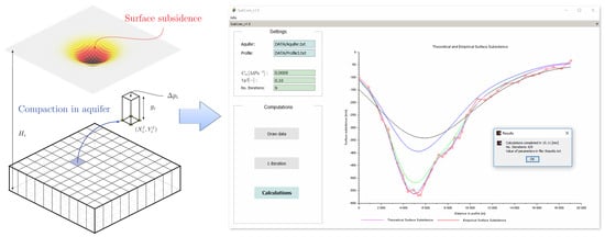
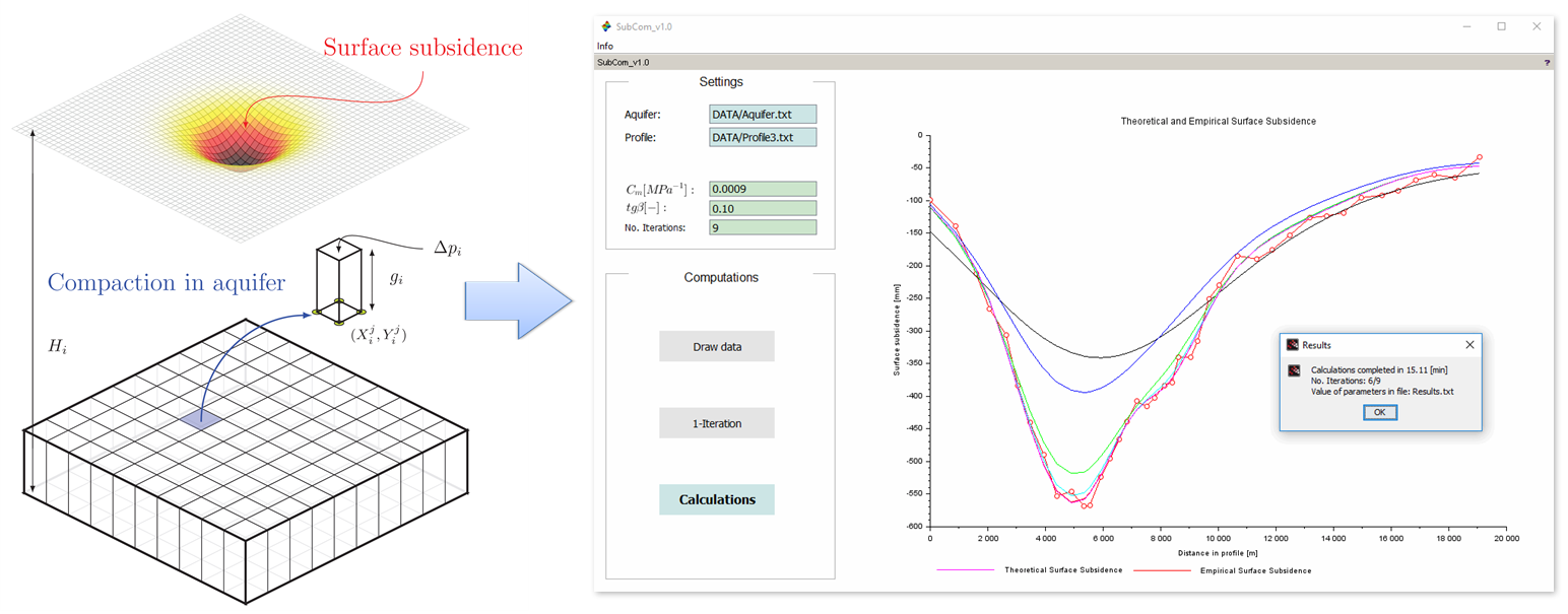
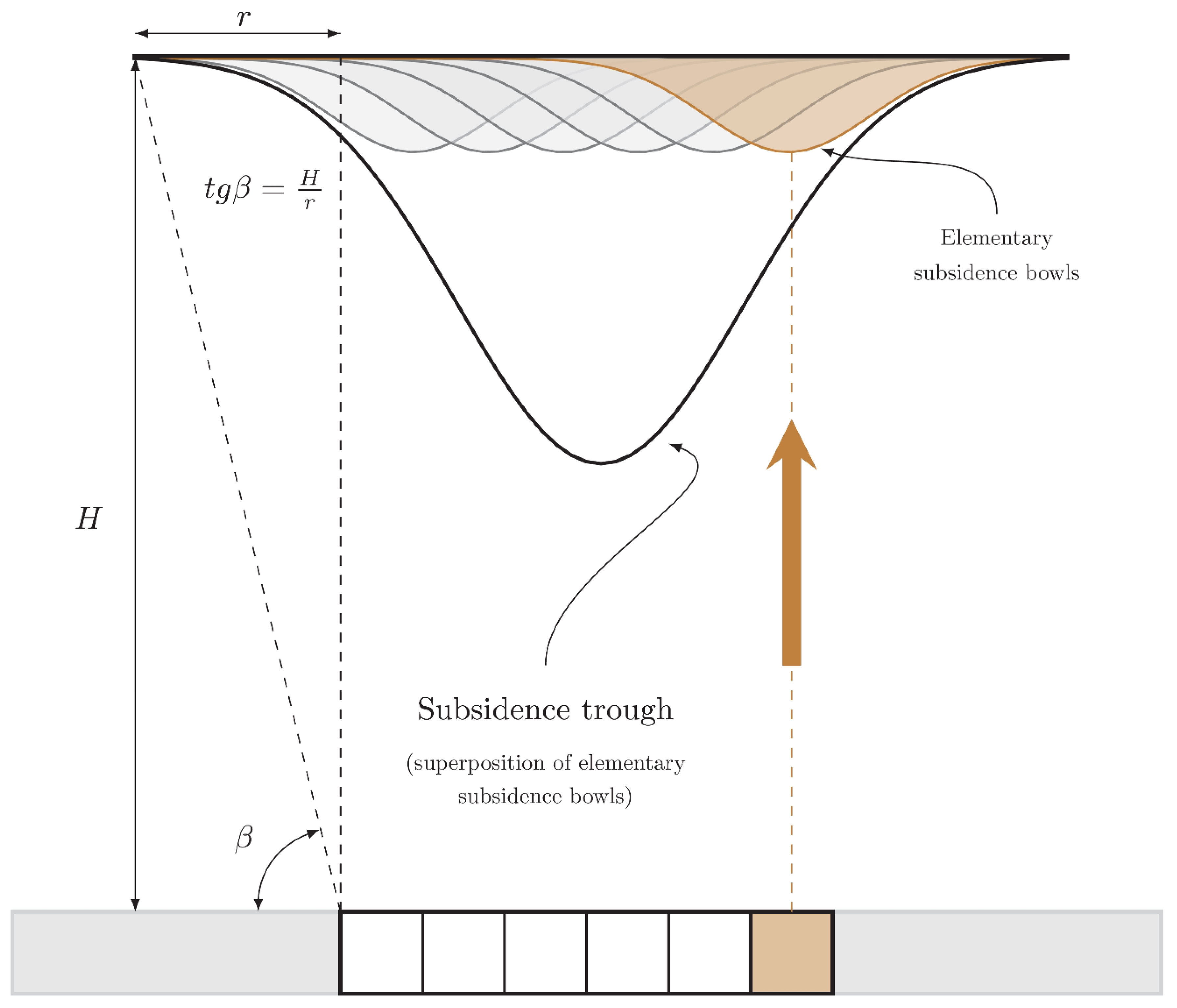
2.1. Principles of a Model Based on the Influence Function

The calculation model presented in the paper is based on the division of a geological structure containing fluid (oil, gas or water) into elementary cuboids, i.e., reservoir elements [13,14]. This aspect is discussed in more detail in Section 2.2. The suggested solution allows reservoir elements to be used in the form of cuboids with arbitrary shaped bases which increase the computational potential of the method [13]. In models based on the influence function, vertical displacements S are the result of the compaction of porous reservoir rocks and may be calculated with Equation (1):

$$S=C_m\left\{p_0-p\left(t\right)\right\}{M}_0{{\displaystyle \iint }}_A^{⬚}\frac{1}{r^2}exp\left(-\pi \frac{R^2}{r^2}\right)dxdy$$

(1)

where Δp = p₀ − p(t)—pore pressure decrease, M₀—primary thickness of layer, A—geometry of reservoir element, R² = (x − s)² + (y − t)²—distance in the horizontal plane between a reservoir element (x,y) and a calculation point on the surface (s,t) and r—radius of influence, which takes the form of:

$$r=\frac{H}{tg\beta }$$

and C_m—compaction coefficient, defined by the expression:

$$C_m=\frac{1}{dp}\frac{dz}{z}$$

(2)

where dp—change in pore pressure, z—initial height of the rock sample, dz—change in the height of the rock sample.

The compaction coefficient (2) is defined as a change in the height of a rock sample z with a corresponding drop in pore pressure dp [27]. In turn, the impact radius r in Equation (1) is associated with reservoir depth H and is directly associated with the mechanical properties of the rocks, which are expressed by parameter tgβ (Figure 1) [37]. Both tgβ and compaction coefficient $C_m$ make up the set of basic parameters of the theoretical model. Their values should correspond with the local conditions in the rock mass. For this reason, determination of these parameters is a basic requirement for credible modeling of surface deformations.

One of the ways of determining parameters ($C_m,tg\beta$) for local conditions is the Gauss-Newton method for nonlinear equation systems. A Taylor series expansion is used to express the original nonlinear equation in linear form, which is the key concept of this technique. An algorithm minimizes the sum of the squares of the residuals between the data and the model. This method has been commonly used to evaluate determined parameters when a sufficient amount of data is available whose values have a relatively low degree of uncertainty [10,38,39,40,41]. By comparing a single empirical observation with a value determined on the basis of the assumed model, the value of error $\delta$ for the ith observation is obtained. The least square method assumes the minimization of the function of error $E$ for n observations (3):

$$E={\displaystyle \sum }_{i=1}^n{\delta }_i{\delta }_i\to minimum$$

(3)

The Gauss-Newton algorithm for the model for Equation (1) was implemented. Owing to the nonlinear equation of the theoretical function, the system of observation equations needs to be linearized, as shown in the Appendix A. The solution requires the assumption of initial values and approximate parameters ($C_{m0},tg{\beta }_0$) for which the increment of ($\Delta C_m,\Delta tg\beta$) is determined. The correct choice of initial parameter values determines the convergence of the solution and the calculation process. The correct application of the least square approach assumes that the testing of outliers in subsidence results has already been performed.

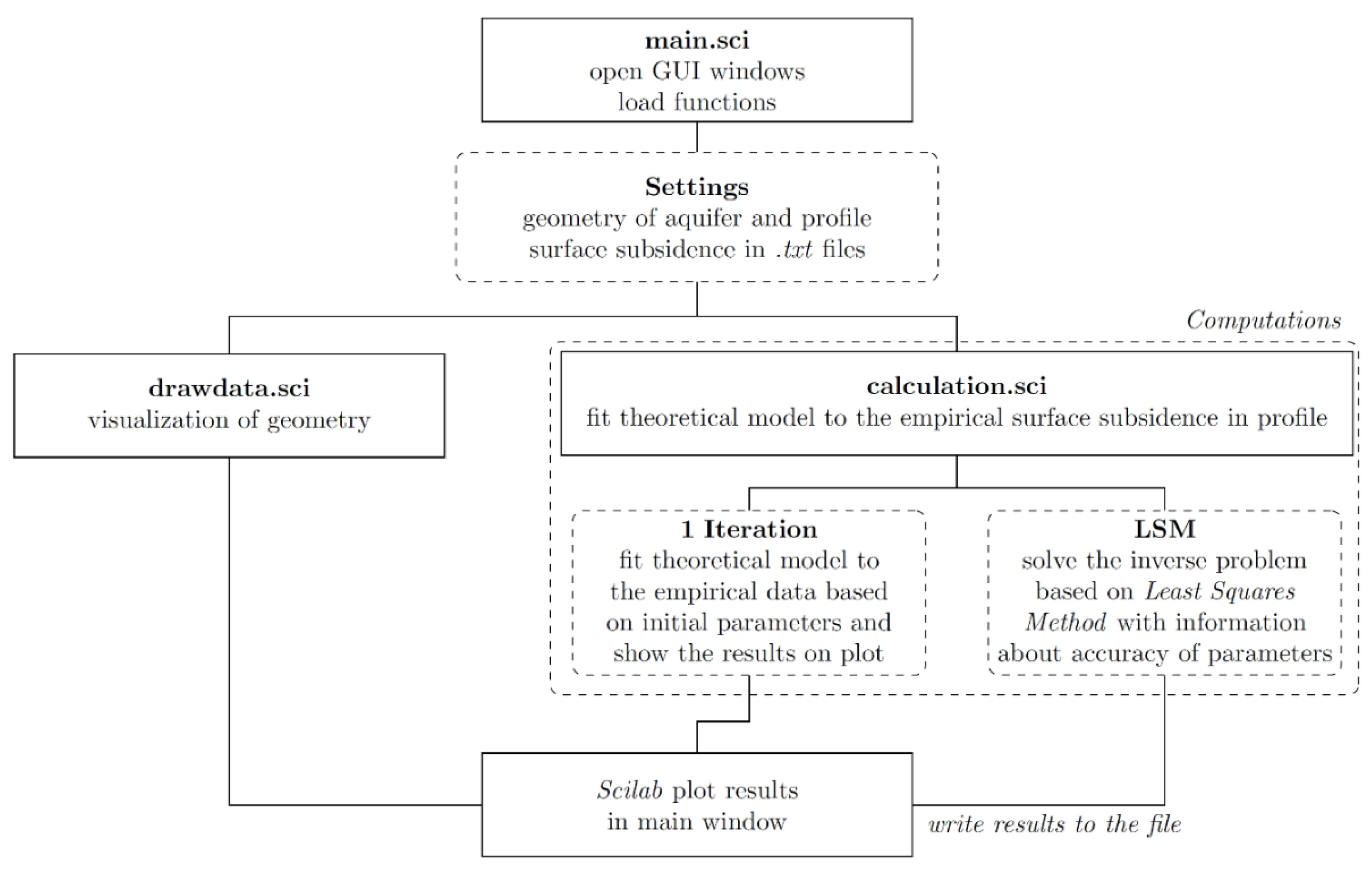
2.2. Program Framework

The presented solution was implemented in the Scilab environment (version 5.5.2); the result was the GUI-based SubCom v1.0 program (Supplementary Materials). Data on vertical surface displacements (e.g., subsidence), the geometry of the aquifer and changes in pore pressure had to be obtained in order to determine the model parameters (

Table 1. Required input data for the SubCom v1.0 program.

Type of Data	Symbol	Description	Data visualization
Profile	Id, X, Y, S	Information about surface subsidence on the profile
Aquifer	$X_i^j,Y_i^j$	The geometry of a single aquifer element in the same coordinate system as the profile
	Hi	Depth
	Mi	The thickness of a single aquifer element
	Δpi	Pressure decrease in the aquifer, determined for the bottom of the aquifer element

). The first set of data contained the number of points (Id), their coordinates (X, Y) and the value of vertical displacements (S). Vertical movements were determined in the subsidence trough profile, which is useful for analyzing results. Another set consisted of geometrical data about the reservoir and data about the pressure drop in a given reservoir element. Such an element had ascribed local values: pressure decrease (Δp_i), thickness (M_i), depth (H_i) and coordinates describing the arbitrary geometry of a single element ($X_i^j,Y_i^j$).

The created graphical user interface simplifies the process of managing the software’s functionality (Figure 2) [42]. The SubCom_v1_0.sce script loads the functions and launches the main window (Figure 3). All plots and graphical presentations are performed with the use of functions in the Scilab environment. The correctness of the prepared data can be verified by visualizing them with the use of drawdata.sci. An error at this stage indicates a problem with the input data. The calculations are based on the initial values of the analyzed parameters. Firstly, the program calculates the theoretical values of vertical deformations with the calculation.sci function; subsequently, a plot showing the fit of the subsidence trough with the theoretical values is obtained (Figure 2). The problem of determining the parameters was solved on the basis of the Gauss-Newton method with a system of observation equations that is described in the Appendix A.

2.3. Calculations for Testing Data

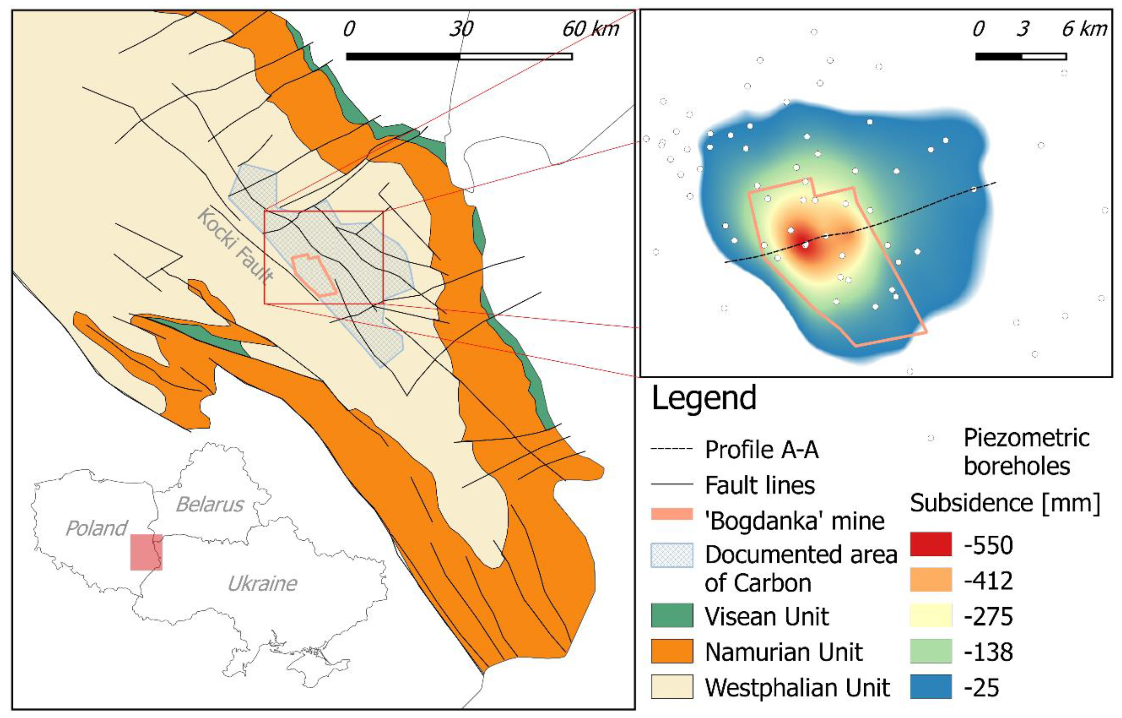
In the first stage, it was decided to validate the results of the implemented solution. The goal was to check the correctness and convergence of the calculations performed. Testing was performed for modeling data. The modeling values of subsidence were disturbed by Gaussian noise. The initial parameter values were changed, and the optimal obtained results were checked (Figure 4). Regardless of the initial calculation parameters, the same final values were obtained for each sample test. In the initial iterations, the convergence of the computational process was stronger than in the subsequent iterations due to a small change in the accepted corrections to the determined values of the parameters. The test confirms the correctness of the algorithm and its implementation in the Scilab environment.

3. Study Area

The presented tool was used on the example of an underground coal mine where aquifer draining resulted in subsidence caused by rock mass compaction.

3.1. Geological Background

There is an underground hard coal mine in eastern Poland where coal has been extracted from Carboniferous beds since the 1980s (Figure 5). These strata are covered by Jurassic, Cretaceous and Quaternary horizons with a total thickness of 500–1400 m. The Carboniferous sediments are directly overlaid by the Jurassic strata, which is 80–120 m thick and consists of sand-limestone sediments from the middle Jurassic period and carbonate sediments from the Upper Jurassic period. The Cretaceous rocks form an almost impervious layer with an average thickness of 470 m. These are mainly marl and limestone strata. The Quaternary sediments generally consist of sandy, clayey material with a thickness of several up to about ten meters [43,44].

The main source of water inflow to the mine is fractures in the Jurassic strata, which consists of carbonate and sandy sediments that are 80 m to 120 m thick. The average water mineralization is about 1292–1583 mg/dm³ with an average water hardness in the range 0.32–0.78 °n. These are very soft waters of the Cl-HCO₃-Na type, whose characteristics should be associated with the fractures and 11–23% porosity. The filtration coefficient of this layer is 10⁻⁸ m/s to 10⁻⁵ m/s, with an average of 10⁻⁶ m/s in the mine area. The primary pressure acting on the top of the Carboniferous layer amounts to approx. 7.5 MPa [43]. The depression cone was monitored with 44 piezometric boreholes located in the vicinity of the mine (Figure 5). Surface deformations could be observed along with the development of the depression cone (Figure 5).

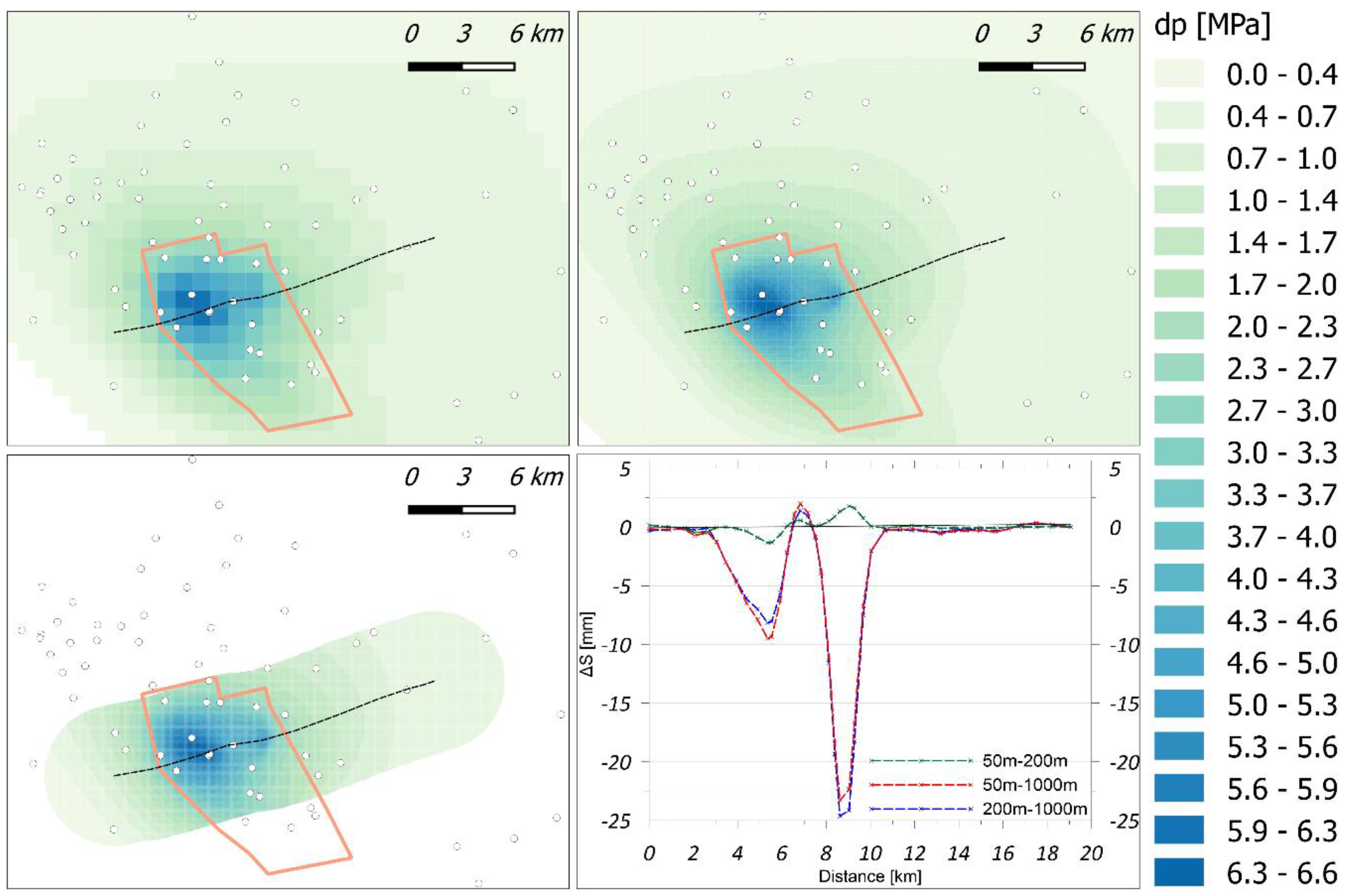
3.2. Subsidence Due To Fluid Withdrawal

The first leveling surveys were performed in the mine area in the 1980s. Vertical deformations of the surface were already observed during the shaft drilling phase. In 1982, the maximum movements in this area reached approximately 0.1 m [5]. At present, deformations can be measured for the whole mine area. A detailed analysis of the leveling results was carried out in 2013 [45]. A more in-depth analysis revealed that the vertical surface movements were caused not only by coal mining operations, but also by draining of deeper geological strata. To determine the range of deformations due to drainage, a network of benchmarks from a national height grid network was located in the neighborhood of the mine. Vertical movements (1980–2011) were determined for 86 common points from the benchmark network. Maximum values of drainage-related movements were observed in the area of shafts, i.e., the main drainage points of the Jurassic strata. The maximum subsidence caused by drainage did not exceed 0.6 m (Figure 5).

4. Results

The SubCom v1.0 software may be used to determine the parameters of fluidal deposits (oil, gas or groundwater). The operation of this program was presented on the case of an underground mine where the compaction of the aquifer led to land-surface subsidence. The calculations were based on 2011 data and 2009 pressure changes in the Jurassic aquifer. The time lapse is due to a 2-year delay in the manifestation of the impact [7].

First, the aspect of the computational size of aquifer elements is discussed (Section 4.1). Finally, the implemented code is used for the case of the underground coal mine example (Section 4.2).

4.1. Dimension Testing Of Aquifer Elements

The assumed method of determining parameters that is referred to in Section 2 is based on dividing the reservoir into elements with ascribed pressure decrease and thickness. Therefore, suitable selection of reservoir element size is very important. The investigated reservoir was divided into cuboid elements whose bases measured 1000, 200 and 50 m (Figure 6). Calculations in profile A-A were conducted for the so-divided aquifer (Figure 6). The calculation results were compared on plots. The determined differences were up to 23 mm for 1000 m bases as compared to their 200 m and 50 m equivalents. The obtained differences in the bases (of 200 m and 50 m) did not exceed 2 mm at a maximum subsidence of 0.56 m with a relative error below 0.5%. Accordingly, it was assumed that the division into elements of the base measuring 200 m was sufficient and optimal for calculation efficiency.

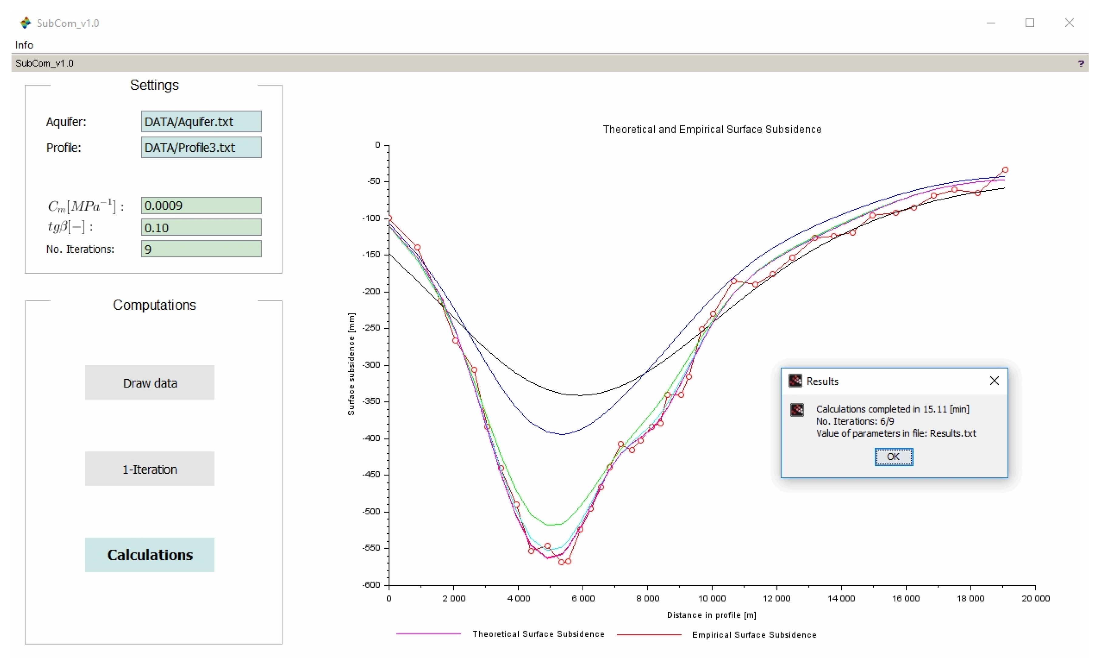
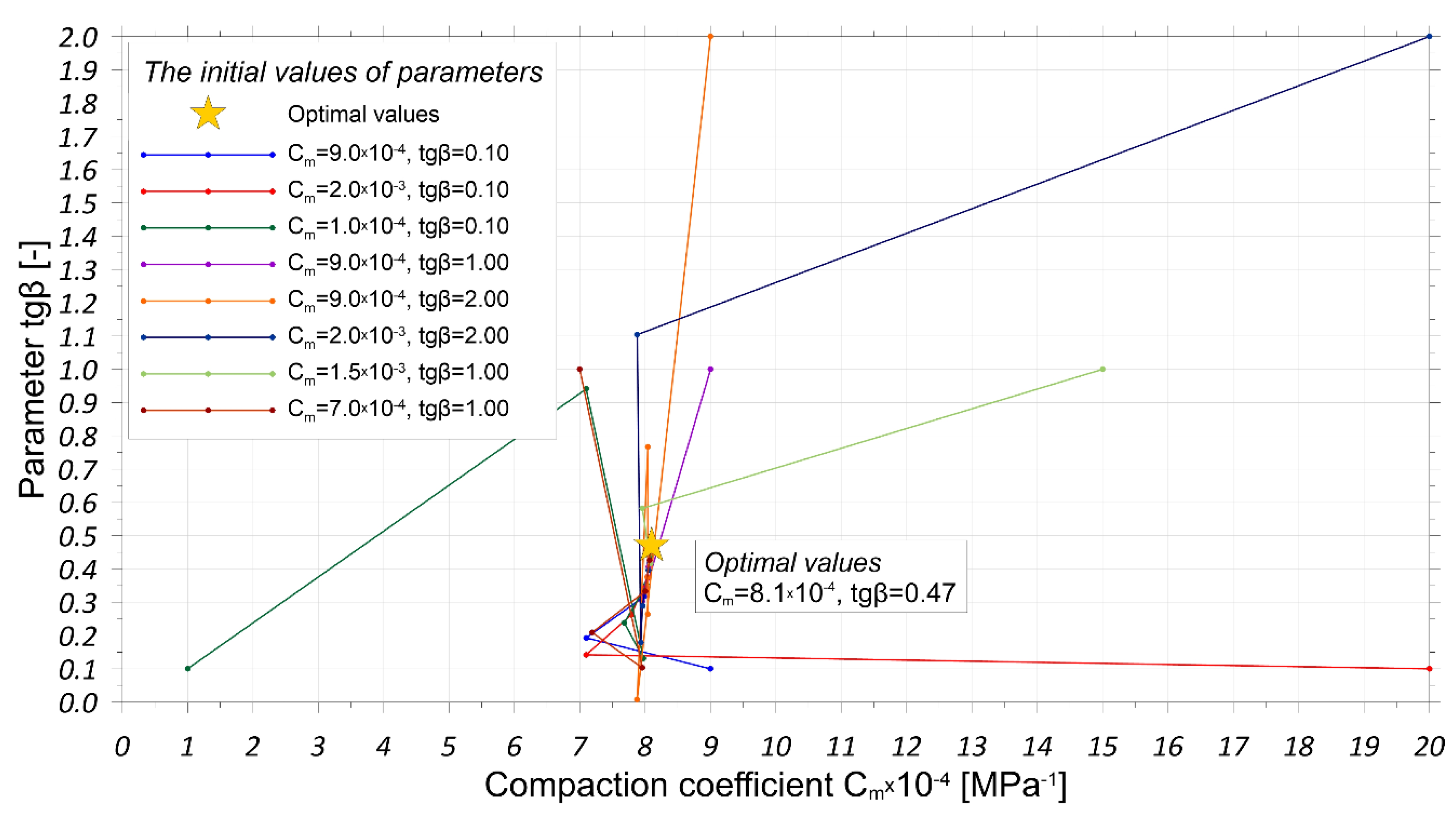
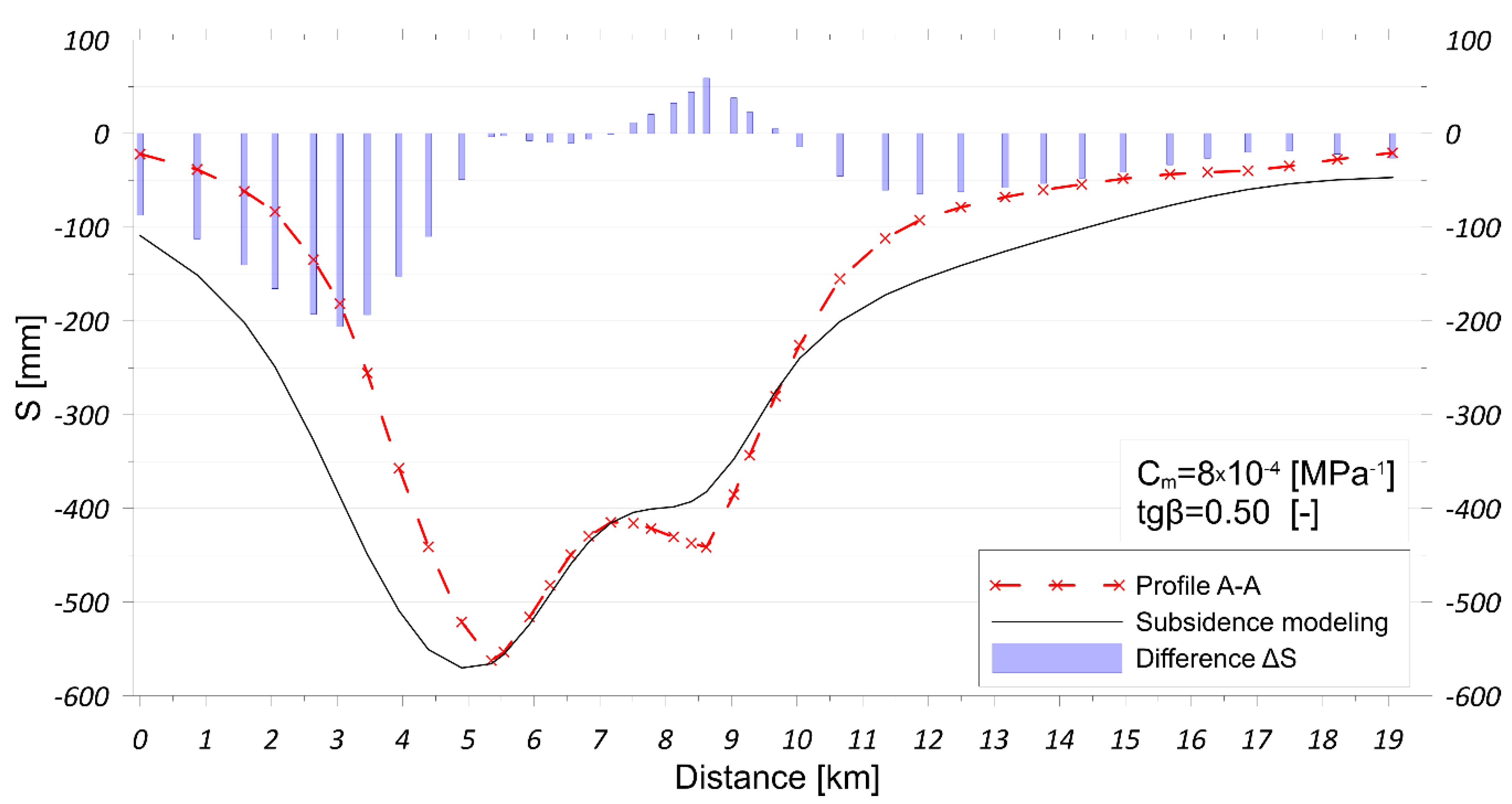
4.2. Estimation Results of Compaction Coefficient C_m and tgβ

The established algorithm allowed parameters C_m and tgβ to be determined. The estimation results in profile A-A and the deviation are shown in Figure 7. The compaction coefficient determined by the software for the Jurassic aquifer was C_m = 8.0 × 10⁻⁴ ± 0.1 MPa⁻¹ at the range expressed by tgβ = 0.50 ± 0.05 at correlation coefficient R² of 0.77. According to Doornhof [46], the compaction coefficient for sandstone may oscillate between 5.0 × 10⁻⁴ MPa⁻¹ and 15.0 × 10⁻⁴ MPa⁻¹, which indicates high reliability of the obtained results. The tgβ value is responsible for the range of surface compaction. For instance, a value of tgβ of 0.10–0.20 was assumed in modeling for the gas field in Groningen, which is located at a depth of over 2000 m [47]. The determined value of tgβ = 0.50 for the Jurassic strata in the coal mine at 500–600 m also seems credible.

5. Discussion and Conclusions

The obtained fitting of the deformation field profile to the modeled values differs along the profile (Figure 7). The biggest discrepancy was observed in the initial part of the cross-section in the Kocki fault area (Figure 5), which constitutes a natural hydrogeological window for waters from the Jurassic horizon. This zone is responsible for the asymmetric shape of the depression cone (Figure 6), which may cause overestimation of vertical deformations in that area. The maximum values of the observed and modeled subsidence are similar, i.e., about 0.56 m, and they can be found in the mine shaft area where the aquifer depression was biggest. The modeled values are underestimated in the section between 7.5 km and 9.5 km of the profile. This is the second shaft drainage area of considerable depression in the reservoir. Due to the lack of piezometric boreholes in that area, the assumed pressure gradient may significantly differ from the real values, which are unknown. This could lead to underestimation of the observed vertical deformation values. The overestimation of modeled values in the eastern part of the mining area may stem from incomplete information about pressure gradients in that part. In the last part of the subsidence trough, where the modeled and observed values are similar, a piezometric well is located.

The proposed method of parameter determination requires the establishment of reservoir elements with the ascribed geometrical information on Δp and H. The pressure gradient in a single element will affect the attained calculation accuracy. An example of a deposit divided into uniform elements with square bases is presented in Section 4. The possibility of using elements with various base sizes is very useful. As shown in the example (Figure 6), this is purposeful, especially in an area of strong local variability of pressure depletion (Δp). Such a solution is possible, and the presented software assumes that reservoir elements may vary in size. However, the proposed model does not assume chemical interactions such as non-equilibrated brines [48]. If it were possible to express the chemical interactions in space (as compaction in Equations (1) and (2)), the model could be expanded. The chemical interactions of rock weakening or chemical effects could be added to the model, and this could be a direction for future research.

The presented SubCom v1.0 software may be used to determine the parameters of a prediction model for areas where groundwater, oil, and gas are extracted. It applies the Scilab open-source environment, in which the graphical interface features of SubCom v1.0 software were created. This software may be used in all locations where a compaction process has been observed. For the sake of calculation, the reservoir has to be divided into reservoir elements which are ascribed a depth and pressure decrease. Initial data for the surface includes subsidence measurement results, which can be obtained with methods such as classic leveling surveys, GNSS, or InSAR. The proposed solution assumes the interpretation of results based on the subsidence trough profile. However, the presented algorithm also allows calculations to be made in a grid of distributed points (3D); although this is not in the scope of the present paper, it may be a starting point for further work on the software and development by users.

References

1. Ketelaar, V.B.H.G. Satellite Radar Interferometry; Remote Sensing and Digital Image Processing 14; Springer: Dordrecht, The Netherlands, 2009; pp. 113–166. [Google Scholar]
2. Osmanoğlu, B.; Dixon, T.H.; Wdowinski, S.; Cabral-Cano, E.; Jiang, Y. Mexico City subsidence observed with persistent scatterer InSAR. Int. J. Appl. Earth Obs. Geoinf. 2011, 13, 1–12. [Google Scholar] [CrossRef]
3. Castellazzi, P.; Garfias, J.; Martel, R.; Brouard, C.; Rivera, A. InSAR to support sustainable urbanization over compacting aquifers: The case of Toluca Valley, Mexico. Int. J. Appl. Earth Obs. Geoinf. 2017, 63, 33–44. [Google Scholar] [CrossRef]
4. Teatini, P.; Tosi, L.; Strozzi, T.; Carbognin, L.; Wegmuller, U.; Rizzetto, F. Mapping regional land displacements in the Venice coastland by an integrated monitoring system. Remote. Sens. Environ. 2005, 98, 403–413. [Google Scholar] [CrossRef]
5. Borowski, W. The development of the subsidence basin in the Central Coal District LZW. Prace Naukowe Politechniki Lubelskiej 1987, 171, 85–105. [Google Scholar]
6. Piestrzyński, A. Monografia KGHM Polska Miedz SA; KGHM CUPRUM Sp. z o.o. CBR: Lubin, Poland, 2008. [Google Scholar]
7. Witkowski, W.T. Modeling of Land Subsidence Due to Hydrological Changes with Artificial Intelligence Tools. Ph.D. Thesis, AGH University of Science and Technology, Kraków, Poland, 2017. [Google Scholar]
8. Galloway, D.; Burbey, T.J. Review: Regional land subsidence accompanying groundwater extraction. Hydrogeol. J. 2011, 19, 1459–1486. [Google Scholar] [CrossRef]
9. Muntendam-Bos, A.G.; Fokker, P.A. Unraveling reservoir compaction parameters through the inversion of surface subsidence observations. Comput. Geosci. 2008, 13, 43–55. [Google Scholar] [CrossRef]
10. Fokker, P.A.; Van Thienen-Visser, K. Inversion of double-difference measurements from optical leveling for the Groningen gas field. Int. J. Appl. Earth Obs. Geoinf. 2016, 49, 1–9. [Google Scholar] [CrossRef]
11. Zoccarato, C.; Ferronato, M.; Teatini, P. Formation compaction vs land subsidence to constrain rock compressibility of hydrocarbon reservoirs. Géoméch. Energy Environ. 2018, 13, 14–24. [Google Scholar] [CrossRef]
12. Witkowski, W.T. Artificial intelligence in modelling of surface subsidence due to water withdrawal in underground mining. In Proceedings of the 15th International Multidisciplinary Scientific GeoConference-SGEM; SGEM2015 Conference Proceedings, Albena, Bulgaria, 18–24 June 2015; pp. 503–510. [Google Scholar]
13. Hejmanowski, R. Zur Vorausberechnung Förderbedingter Bodensenkungen Über Erdöl-und Erdgaslagerstätten. Ph.D. Thesis, Technische Universität Clausthal, Clausthal, Germany, 1993. [Google Scholar]
14. Sroka, A.; Hejmanowski, R. Subsidence prediction caused by the oil and gas development. In Proceedings of the 3rd IAG Symposium on Geodesy for Geotechnical and Structural Engineering and 12th FIG Symposium on Deformation Measurements, Baden, Germany, 22–24 May 2006. [Google Scholar]
15. Hejmanowski, R.; Malinowska, A. Evaluation of reliability of subsidence prediction based on spatial statistical analysis. Int. J. Rock Mech. Min. Sci. 2009, 46, 432–438. [Google Scholar] [CrossRef]
16. Malinowska, A. A fuzzy inference-based approach for building damage risk assessment on mining terrains. Eng. Struct. 2011, 33, 163–170. [Google Scholar] [CrossRef]
17. Terzaghi, K. Settlement and Consolidation of Clay; McGraw Hill: New York, NY, USA, 1925; pp. 874–878. [Google Scholar]
18. Biot, M.A. General Theory of Three-Dimensional Consolidation. J. Appl. Phys. 1941, 12, 155–164. [Google Scholar] [CrossRef]
19. Poland, J.F. Guidebook to Studies of Land Subsidence Due to Ground-Water Withdrawal; UNESCO: Paris, France, 1984. [Google Scholar]
20. Brown, K.; Trott, S. Groundwater Flow Models in Open Pit Mining: Can We Do Better? Mine Water Environ. 2014, 33, 187–190. [Google Scholar] [CrossRef]
21. Fokker, P.A.; Orlić, B. Semi-Analytic Modelling of Subsidence. Math. Geol. 2006, 38, 565–589. [Google Scholar] [CrossRef]
22. Knothe, S. A profile equation for a definitely shaped subsidence through. Arch. Min. Sci. 1953, 1, 22–38. [Google Scholar]
23. MSEC. Methods of Subsidence Prediction; Unpublished report by Mine Subsidence Engineering Consultants; MSEC: Chatswood, Australia, 2008. [Google Scholar]
24. Diaz-Fernandez, M.E.; Álvarez-Fernández, M.I.; Álvarez-Vigil, A.E. Computation of influence functions for automatic mining subsidence prediction. Comput. Geosci. 2009, 14, 83–103. [Google Scholar] [CrossRef]
25. Sroka, A.; Schöber, F. Studie zur Analyse und Vorhersage der Bodensenkungen und des Kompaktionsverhaltens des Erdgasfeldes Groningen/Emsmündung; Abschlussbericht: Clausthal-Zellerfeld, Germany, 1990. [Google Scholar]
26. Hoffmann, J.; Galloway, D.; Zebker, H.A. Inverse modeling of interbed storage parameters using land subsidence observations, Antelope Valley, California. Water Resour. Res. 2003, 39. [Google Scholar] [CrossRef]
27. Zhang, M.; Burbey, T.J. Inverse modelling using PS-InSAR data for improved land subsidence simulation in Las Vegas Valley, Nevada. Hydrol. Process. 2016, 30, 4494–4516. [Google Scholar] [CrossRef]
28. McGovern, S.; Kollet, S.; Bürger, C.M.; Schwede, R.L.; Podlaha, O.G. Novel basin modelling concept for simulating deformation from mechanical compaction using level sets. Comput. Geosci. 2017, 148, 835–848. [Google Scholar] [CrossRef] [Green Version]
29. Feng, X.-T.; Hudson, J.A. Specifying the information required for rock mechanics modelling and rock engineering design. Int. J. Rock Mech. Min. Sci. 2010, 47, 179–194. [Google Scholar] [CrossRef]
30. Geertsma, J. Land Subsidence Above Compacting Oil and Gas Reservoirs. J. Pet. Technol. 1973, 25, 734–744. [Google Scholar] [CrossRef]
31. Fokker, P.A.; Osinga, S. On the Use of Influence Functions for Subsidence Evaluation. In Proceedings of the 52nd U.S. Rock Mechanics/Geomechanics Symposium, Seattle, WA, USA, 17–20 June 2018. [Google Scholar]
32. Knothe, S. Prediction of Influence Mining Exploitation; Śląsk: Katowice, Poland, 1984. [Google Scholar]
33. Hebblewhite, B.; Waddington, A.A.; Wood, J.H. Regional horizontal surface displacements due to mining beneath severe surface topography. In Proceedings of the 19th International Conference on Ground Control in Mining, Morgantown, WV, USA, 8–10 August 2000. [Google Scholar]
34. Ren, G.; Li, G.; Kulessa, M. Application of a Generalised Influence Function Method for Subsidence Prediction in Multi-seam Longwall Extraction. Geotech. Geol. Eng. 2014, 32, 1123–1131. [Google Scholar] [CrossRef]
35. Ren, G.; Buckeridge, J.; Li, J. Estimating Land Subsidence Induced by Groundwater Extraction in Unconfined Aquifers Using an Influence Function Method. J. Water Resour. Plan. Manag. 2015, 141, 04014084. [Google Scholar] [CrossRef]
36. Kraemer, S. Analytic Element Ground Water Modeling as a Research Program (1980 to 2006). Ground Water 2007, 45, 402–408. [Google Scholar] [CrossRef] [PubMed]
37. Hejmanowski, R. Modeling of time dependent subsidence for coal and ore deposits. Int. J. Coal Sci. Technol. 2015, 2, 287–292. [Google Scholar] [CrossRef] [Green Version]
38. Kwinta, A.; Gradka, R. Analysis of the damage influence range generated by underground mining. Int. J. Rock Mech. Min. Sci. 2020, 128, 104263. [Google Scholar] [CrossRef]
39. Samsonov, S.; Van Der Kooij, M.; Tiampo, K. A simultaneous inversion for deformation rates and topographic errors of DInSAR data utilizing linear least square inversion technique. Comput. Geosci. 2011, 37, 1083–1091. [Google Scholar] [CrossRef]
40. Maciuk, K. GPS-only, GLONASS-only and combined GPS+GLONASS absolute positioning under different sky view conditions. Tehnički Vjesnik 2018, 25, 933–939. [Google Scholar]
41. Malinowska, A.; Hejmanowski, R.; Dai, H. Ground movements modeling applying adjusted influence function. Int. J. Min. Sci. Technol. 2020, 30, 243–249. [Google Scholar] [CrossRef]
42. Dey, S.; Singh, A.K.; Prasad, D.K.; McDonald-Maier, K.D. SoCodeCNN: Program Source Code for Visual CNN Classification Using Computer Vision Methodology. IEEE Access 2019, 7, 157158–157172. [Google Scholar] [CrossRef]
43. Wilk, Z. Hydrogeologia Polskich Złóż Kopalin i Problemy Wodne Górnictwa—Tom 1; Uczelniane Wydawnictwa Naukowo-Dydaktyczne AGH: Kraków, Poland, 2003. [Google Scholar]
44. Paczyński, B.; Sadurski, A. Polish Regional Hydrogeology: Volume II—Mineral, Curative and Thermal Waters as Well as Mining Waters; Państwowy Instytut Geologiczny: Warszawa, Poland, 2007. [Google Scholar]
45. Hejmanowski, R.; Sopata, P.; Stoch, T.; Wójcik, A.; Witkowski, W.T. Impact of coal rock mass drainage on surface subsidence. Przeglad Górniczy 2013, 69, 38–43. [Google Scholar]
46. Doornhof, D.; Kristiansen, T.G.; Nagel, N.B.; Pattillo, P.D.; Sayers, C. Compaction and Subsidence. Oilfield Rev. 2006, 18, 50–68. [Google Scholar]
47. Sroka, A.; Tajduś, K. Calculating land subsidence in the exploitation of oil and gas. Wiertnictwo Nafta Gaz 2009, 26, 327–335. [Google Scholar]
48. Austad, T.; Strand, S.; Madland, M.V.; Puntervold, T.; Korsnes, R.I. Seawater in Chalk: An EOR and Compaction Fluid. SPE Reserv. Evaluation Eng. 2008, 11, 648–654. [Google Scholar] [CrossRef]
Figure 1. The idea of a computational model based on the influence function and graphical interpretation of the tgβ parameter. The dark orange arrow visualizations the influence function, which represents the deformation process in rock mass.
Applsci 10 03287 g001
Figure 2. The main window of SubCom v1.0, showing the results of computation.
Applsci 10 03287 g002
Figure 3. The framework of the SubCom v1.0 program.
Applsci 10 03287 g003
Figure 4. Determination of optimal parameter values related to different initial conditions. The testing was carried out for modeling data; optimal parameters are represented by a star on the graph. The iterations are represented by colored dots on each track.
Applsci 10 03287 g004
Figure 5. Location of the hard coal mine and the regional tectonics of the area. Piezometric boreholes and a large dewatering trough in the deep extraction area are shown. Condition as of 2011.
Applsci 10 03287 g005
Figure 6. Division of aquifer into cuboid reservoir elements whose bases measured 1000 m, 200 m, and 50 m. Owing to the large number of base elements measuring 50 m, a buffer was used for profile A-A. Changes in reservoir element pressure are shown in the color scale.
Applsci 10 03287 g006
Figure 7. Fitting the model to the A-A dewatering trough profile with a plot of differences.
Applsci 10 03287 g007