Comparative Performance of a Hybrid Renewable Energy Generation System with Dynamic Load Demand

Abstract

This article presents the modeling and simulation of a hybrid generation system, which uses solar energy generation, wind energy, and the regulation of a proton exchange membrane (PEM) cell to raise the demanded load, empowering the use of these hydride systems worldwide. This generation system was simulated for different locations in Puerto Bolivar (Colombia), Bremen (Germany), Beijing (China), and Texas (USA), for two demand profiles. The data used for the simulation was calculated using the mathematical solar model proposed by Beistow and Campbell for solar radiation. In contrast, for the wind resource evaluation, the Weibull probability distribution was used to calculate the most probable wind speed for each day, according to the historical data for each of the studied locations. Considering these data, the process transfer functions were used for tuning the control parameters for the hydrogen and oxygen production system. For the evaluation of the performance of these controllers, the indices of the absolute value of the error (IAE), the integral of the square of the error (ISE), the integral of the absolute value of the error for time (ITAE), and the integral of the square of the error for time (ITSE) were used. It was found that in the second load profile studied, better performance of the ITSE performance parameter was obtained, with stabilization times lower than those of the first profile.

1. Introduction

Global energy consumption has increased significantly due to population growth [1]. The increase in energy demand has prompted the search for alternatives for energy generation, the development of thermal processes according to the rational use of energy, preservation of the environment [2], and the improvement of thermal efficiency by mean of thermoeconomics modeling [3] and thermoeconomic optimization [4]. The development of new-generation systems using renewable energies has been one of the most widely studied options [5,6] because many countries have developed an energy policy that encourages the generation of environmentally friendly options based on clean-development mechanisms [7]. Thus, the contribution of these energy sources globally has been growing. Between 2016 and 2017, as recorded by Bloomberg New Energy Finance (BNEF), there was an increase in renewable energy of 2%, which equates to a rise of almost 157 GW in global power generation [8].

Electricity production from solar energy increased from 1050 GW in 1992 to 112,150 GW by 2013. Of this increase, 78% was produced by Japan, the United States, Germany, Spain, and Italy [9]. This was achieved thanks to various projects that were developed in different countries. In South Korea, a neural network model was built to calculate horizontal solar irradiation, taking images from the Korean communication, ocean, and meteorological satellites (COMS) as input; this model has an error of 12% and a correlation coefficient of 0.975. The result of this model was the generation of hour-by-hour solar radiation maps in South Korea [10]. Similarly, in Saudi Arabia, taking into account that this government wants to invest USD 109 billion over the next 20 years, a document was presented that assesses if there is potential for generating photovoltaic energy in homes. The results for two typical building structures in the country were analyzed, taking into account the demands for electricity of these buildings, and a cost–benefit assessment for different scenarios of photovoltaic systems was completed [11].

On the other hand, wind energy has also been developed as a good alternative to fossil fuels for energy generation. This is reflected in research that shows that in the United States, there was an increase in the production of wind energy of approximately 14% between 2004 and 2013. Similarly, Germany and China presented increases in wind energy production, reaching approximate increases of 8% and 7.7%, respectively, for the same period [12]. A recent study looked at the Changhua-South Offshore Wind Farm by using data obtained from a meteorological mast, a detection device, and a floating light range (LiDAR); these data were collected by the NASA Climate Simulation Center. The results of this assessment showed that at a height of 105 m, wind speeds were 7.97 and 8.02 m/s, from the floating LiDAR device and mast, respectively, and produced the potential of up to 314 GWh/year [13]. Likewise, for Latin America, 141 locations in the Gulf of Mexico were analyzed by calculating the main characteristics of the wind. Hourly records from 1980 to 2017 were analyzed at a height of 50 m, using the free software R, and showed that different locations had different good wind seasons; for fall, winter, and spring, the states of Tamaulipas, Veracruz, and Tabasco were good for wind energy production, while Campeche and Yucatan were good in winter and spring [14]. Despite this, low wind power has presented some difficulties for the development of wind energy production. This is mainly due to the low wind speeds and higher turbulence that occur in built environments due to the presence of obstructions. This turbulence causes fatigue in the turbines, which generates a decrease in their useful life, leading to an increase in maintenance costs [15]. Similarly, it has been demonstrated that the use of low-scale, wind–solar systems represents a financial risk [16].

Another alternative energy source is hydrogen, and this fuel has been the focus of studies in recent years. In the 2000s, research on this topic increased annually by 18% on average, and most of the papers presented were journal articles [17]. However, one of the biggest challenges in using hydrogen as an energy source is the difficulty in storing it. For this reason, many works have focused on this problem. Between 2009 and 2018, 72.3% of all published literature on hydrogen cells focused on storage. In addition, the United States is the country with the most significant influence on hydrogen storage, even though China is the country that has published the most significant number of papers on this subject [18]. Studies have also been carried out in which hybrid systems have been analyzed. These systems have been applied to electric vehicles, achieving an average consumption with a hydrogen cell of 3.7 kWh and 1.12 kg/100 km for hydrogen consumption [19]. Similarly, hybrid systems made up of wind and solar generation, and the use of hydrogen cells have been evaluated. The authors of [20] proposed a model that integrated a horizontal axis wind turbine and a solar panel system. PVC tubes were used as the material to construct the wind turbine blades. That work proposed the integration of two emerging energy systems based on non-conventional energy sources, through a load controller and an inverter for the energy supplied to the residential level [20]. In addition, a smart energy hybrid generation system was studied, which integrated a fuel cell stack, a wind turbine, and a solar panel system. The results obtained in this study show that in the winter, the integration of the system with a wind source provides better performance than the solar system alone. The wind turbine produced 16 kW during January, while the solar system generated 2 kW during the same period. In June, the solar thermal system generated 17 kW, and the wind turbine only 11 kW, which means that the studies of these systems must be carried out for an entire year [21].

The optimal design through optimization algorithms was studied for hybrid energy generation systems based on solar and wind sources, considering three search algorithms to improve the accuracy of the results. In that study, solar radiation was predicted from meteorological variables such as ambient temperature and wind speed with artificial neural network architecture. Thus, the size of the systems must be considered to determine the economic viability of these systems [22].

These hybrid systems have presented promising results. The authors of [23] created a system that has a solar heliostat field, a wind turbine, and a copper-chlorine thermochemical cycle for hydrogen production. In this system, the solar heliostat field was used as a thermal energy source, and the wind system was used to generate the electrical energy necessary for electrolysis and the compressors of the hydrogen storage system. This system was modeled and simulated, obtaining high hydrogen production rates and an overall system efficiency of up to 49% [23].

The main contribution of this paper is to present the comparative performance analysis of hybrid renewable energy generation systems under different load demands, located in areas with the greatest wind and solar potential in Colombia. In addition, meteorological data to calculate mathematical models were used to predict the solar radiation and statistical probability methods for the wind speed prediction in the selected areas. Simulating the system is expected to test the operational planning, the renewable energy complementarity of this system in the selected areas, and the feasibility of using the proton exchange membrane (PEM) cell as a support to the hybrid renewable system at those times of the year when wind and solar valleys are present. Likewise, some performance indicators of the proportional integral derivative (PID) control system based on the error calculation are evaluated under two energy demand profiles. The evaluated performance indicators include the absolute value of the error (IAE), the integral of the square of the error (ISE), the integral of the absolute value of the error for time (ITAE), and the integral of the square of the error for time (ITSE).

2. Methodology

The following are the geographic locations used in this work. These were selected based on the availability of data and variable environmental conditions. Similarly, the data obtained in these areas and the description of the generation process are presented together with the control systems. In addition, the mathematical models applied to the solar panel, the wind turbine, and the hydrogen cell are presented; these models were used for the simulation of the hybrid generation system.

2.1. Description and Information About the Region

For the evaluation and comparison of the hybrid trigeneration system, four countries were selected: USA, Germany, China, and Colombia. The first three countries were chosen for their great influence on their continents; on the other hand, Colombia was chosen because it is the country in which the study was carried out. According to the report of the National Renewable Energy Laboratory (NREL) of the United States, the central region of the Central American country has the greatest wind potential [24], i.e., the state of Texas, USA, which is why Texas was chosen for the current study. A study by Germany’s federal environment agency also showed that the northern part of Germany, which includes the cities of Berlin, Bremen, and Hamburg, among others, is the area with the greatest wind power generation capacity. This is the reason why the city of Bremen was chosen for the current study [25]. Similarly, for the selection of the Chinese city in this study, an investigation on the wind speed pattern was taken into account, and it was found that the eastern part of China, in which Beijing is located, has great wind potential, so Beijing was chosen for the current study [26]. Finally, for Colombia, the department chosen was Guajira, taking into account the wind atlas of this country [27]. Figure 1 shows the coordinates where the data on solar irradiation and wind speed were collected.

The wind speed and solar radiation data were obtained using the methodology set out in Section 2.4, with an hourly frequency, and correspond to a one-year interval, starting on 1 January 2019, and ending on 31 December of the same year. The wind speed data were calculated for a height of 50 m for the simulation.

2.2. System Description

The hybrid power generation system, presented in Figure 2, consists of a wind turbine and a solar panel. These two primary sources of generation feed the load demanded by the system. When the climatic conditions of the area are not sufficient to cover the demand, the hydrogen cell comes into operation to supplement the missing energy. Due to climatic conditions, excess energy may be used for the electrolysis of the water in the hydrogen cell. Figure 2 shows the schematic layout of the generation system studied. The input and output in the hydrogen cell system are managed by a proportional integral derivative (PID) control system, in which a constant load is used as a set point to facilitate the calculations.

2.3. Model Description

To carry out the simulation of the hybrid trigeneration system, a mathematical model was made for each of the three energy sources used in the work. Solar energy is obtained through the photovoltaic method, which transforms direct solar radiation into electrical energy through panels. The model adopted to simulate the photovoltaic solar panel was based on the studies conducted by Pandiarajan and Muthu [28]. All of the relevant phenomena in the modeling of a photovoltaic panel are shown in

Table 1. Photovoltaic panel model.

Variable	Model
Light generated current in a PV module,$I_{ph}$ [A]	$I_{ph}=\frac{\lambda · \left(I_{SCr}+K · T-298 · K\right)}{100}$(1)
Inverse saturated current, $I_{rs}$ [A]	$I_{rs}=\frac{I_{SCr}}{e^{\frac{q · V_{OC}}{N_s · k · A · T}}-1}$(2)
Saturation current, $I_O$ [A]	$I_O=I_{rs}·{\left(\frac{T}{T_r}\right)}^3·e^{\frac{q·E_{go}}{Bk}·\left(\frac{1}{T_r}-\frac{1}{T}\right)}$(3)
Cell output current, $I_{pv}$ [A]	$I_{pv}=N_P· I_{ph}-N_P·I_o·e^{\frac{q · \left(V_{pv}+I_{pv} ·R_S\right)}{N_{s }· k · A · T}-1}$(4)

.

In this model, the light generated current in a PV module is calculated from the Equation (1), and the inverse saturated current is defined from the Equation (2). Furthermore, it is taken into account that the saturation current varies with the temperature of the panel, for which it is modeled and expressed, as seen in Equation (3). In Equation (4), the cell output current is described. The photovoltaic panel model allows us to describe mathematically the operation of the panel array included in the system studied and to observe its curves of current–voltage and power–voltage operating under standard conditions. The simulation allows for the observation and analysis of one or more variables as a function of time, where the input variable to the system is the annual radiation profile in the selected places, and the main output is power generated, which is regulated in the hybrid generation system according to the energy load profile. The parameters required for the simulation were obtained from the literature and technical information provided by the manufacturer of the equipment [28].

Similarly, wind energy is transformed into electrical energy by a turbine, which transforms the kinetic energy of the wind into rotational energy by the propellers. In turn, this rotational energy is transformed into electrical energy by a generator. The dynamic model used for the analysis in the simulation was the one presented by Khan and Iqbal [29], which is expressed in Equation (5).

$$\frac{y\left(s\right)}{x\left(s\right)}=\frac{0.25}{s^2+0.7·s+0.25}$$

(5)

This model was developed for a Southwest Wind Power Inc. AIR 403 wind turbine. The power generated varies with wind speed and behaves as described in Figure 3.

The power generation capacity of this turbine has a maximum speed limit of 40 miles per hour. At or above this wind speed, power generation becomes impossible. For the hydrogen cell, the model uses the expanded form of the Nemst Equation [30], which models the thermodynamic potential E and is presented in

Table 2. Proton exchange membrane (PEM) fuel cell model.

Variable	Model
Thermodynamic potential, E [V]	$E=1.229-0.00085·\left(T-298.15\right)+4.3085·{10}^{-5}T·\left[ln\left(p_{h_2}\right)+0.5·ln\left(p_{o_2}\right)\right]$(6)
Oxygen concentration, $C_{O_2}$ [mol/m3]	$C_{O_2}=\frac{P{o}_2}{5.8·{10}^6·e^{\raisebox{1ex}{$-498$}\!\left/ \!\raisebox{-1ex}{$T$}\right.}}$(7)
Overvoltage activation, $n_{act}$ [V]	$n_{act}=-0.96514+0.00312T-0.000187·\ln \left(i\right)+74-5T·\ln \left(C_{O_2}\right)$(8)
Internal resistance, $R_{int}$ [Ω]	$R_{int}=0.01605-3.5·{10}^{-5}T+8·{10}^{-5}·i$(9)
PEM output voltage, $V$ [V]	$V=E-V_{act}+{\mathsf{ῃ}}_{ohmic}$(10)
Hydrogen production rate, $n_{H_2}$ [mol/s]	$n_{H_2}=\frac{n_F·n_c·i_e}{2F}$(11)

as Equation (6). As for the concentration of dissolved oxygen at the gas–liquid interface, the Henry Law model [31] is used, which is shown in the table as Equation (7).

In addition, this model takes into account the excess voltage caused by the activation and the internal resistance, whose models were developed experimentally and are presented in Equations (8) and (9), respectively. Similarly, the output voltage of the fuel cell is modeled according to Equation (10), and the hydrogen production rate, according to Faraday’s law, is presented in Equation (11).

A more detailed description of the models adopted for the development of this study can be found in the literature. The dynamic model of the fuel cell [32] is a function of the external fuel and the oxidant supply; in other words, as long as both flows are fed continuously and in equivalent proportions, the fuel cell will operate correctly in the hybrid energy generation system, which is regulated by means of the PID controller. This cell is composed of two electrodes: an anodic side in which hydrogen is fed, and a cathodic side in which oxygen is fed. The two electrodes act as platinum catalysts and are separated by a thin membrane of an electrolytic ionic conductor. The cell considered in this dynamic model in this research is a PEM (proton exchange membrane or electrolytic polymer membrane), which allows protons to flow through the cell, but stops the movement of electrons, reactants, and products through the cell [29].

2.4. Control System Description

For the control system of the hybrid generation system, steady-state operational values are required. These values were defined for both the fuel cell and the photovoltaic cell based on research results presented in the literature [32]. The values for the fuel cell are presented in

Table 3. Steady-state values for the fuel cell.

Parameters	Values	Parameters	Values
Gas constant	0.0821 L$·$atm/mol K	Cell PEM output current	8.26 A
Faraday constant	96 500 C/mol	PEM output voltage	48 V
Heat capacity	10 000 J/°C	PEM cell power	401.23 W
Anode temperature	25 °C	Molar hydrogen flow	0.005 mol/s
Thermal resistance	0.04 °C/W	Molar oxygen flow	0.005 mol/s
Capacitance	108.75 μF	Demanded charge power	200 W
Cathode resistance	4 mΩ	-	-
Resistance of a PV module	0.01 Ω	-	-

.

For the photovoltaic cell, the assigned constant values are presented in

Table 4. Constants for the Photovoltaic cell.

Variables	Values
Rated power	37.08 W
Voltage in maximum power point, (Vmp)	16.56 V
Current in maximum power point, (Imp)	2.25 A
Open circuit voltage, (VOC)	21.24 V
Short-circuit current, (ISCr)	2.55 A
Total number of cells in series, ($N_s$)	36
Total number of cells in parallel, ($N_p$)	1

.

A PID control is used to control the hybrid system, and the tuning of these controllers was done using the Ziegler–Nichols open-loop method [33]. The approach of the plant to a first-order process plus dead time was made by a set of open-loop tests.

First, the gain, tao, and dead time were determined for the first-order equation, following the procedures outlined in Smith and Corripio [34]. The procedure was performed for a variation in the hydrogen flow rate from 0.005 to 0.008 mol/s while keeping the oxygen flow constant. Then, the oxygen flow rate was changed while keeping the hydrogen flow constant. The transfer functions obtained for hydrogen and oxygen are presented in Equations (12) and (13), respectively.

$$G{\left(S\right)}_{\mathrm{oxygen}}=\frac{125· e^{-1.21s}}{18.20· s+1}$$

(12)

$$G{\left(S\right)}_{\mathrm{hydrogen}}=\frac{62· e^{-0.21s}}{23.22· s+1}$$

(13)

Having obtained the values, tuning was carried out using the Ziegler–Nichols rules [35], resulting in the tuning parameters for the oxygen and hydrogen PID controllers shown in

Table 5. Controller tuning parameters.

	${\mathit{K}}_{\mathit{C}}$	${\mathit{T}}_{\mathit{i}}$	${\mathit{T}}_{\mathit{d}}$	$\mathit{t}/{\mathit{t}}_{\mathit{o}}$
Oxygen	0.14409	2.426	0.606	0.067
Hydrogen	21.155	0.425	0.10625	0.009

.

To evaluate the performance of the PIDs for the different load profiles, four indices were used to calculate the time taken to reach system stabilization [36]. The first index is defined by the integral of the square of the error, as seen in Equation (14).

$$\mathrm{ISE}={\displaystyle \sum }_{\mathrm{I}=2}^{\mathrm{n}}{{\displaystyle \int }}_0^{\mathrm{tsim}}{\left({\mathrm{w}}_{\mathrm{i}}-{\mathrm{w}}_1\right)}^2\mathrm{dt}$$

(14)

Similarly, the integral of the absolute error is given by Equation (15).

$$\mathrm{IAE}={\displaystyle \sum }_{\mathrm{I}=2}^{\mathrm{n}}{{\displaystyle \int }}_0^{\mathrm{tsim}}\left|{\mathrm{w}}_2-{\mathrm{w}}_1\right|\mathrm{dt}$$

(15)

Likewise, the integral of the time-weighted absolute error is described according to Equation (16).

$$\mathrm{ITAE}={\displaystyle \sum }_{\mathrm{I}=2}^{\mathrm{n}}{{\displaystyle \int }}_0^{\mathrm{tsim}}\mathrm{t}· \left|{\mathrm{w}}_{\mathrm{i}}-{\mathrm{w}}_1\right|\mathrm{dt}$$

(16)

Finally, the integral of the time-weighted squared error is defined by Equation (17).

$$\mathrm{ITSE}={\displaystyle \sum }_{\mathrm{I}=2}^{\mathrm{n}}{{\displaystyle \int }}_0^{\mathrm{tsim}}\mathrm{t}· {\left({\mathrm{w}}_{\mathrm{i}}-{\mathrm{w}}_1\right)}^2\mathrm{dt}$$

(17)

where $t_{sim}$ is the simulation elapsed time, n represents the number of iterations, and w is the output values in each iteration executed.

2.5. Data Resources

One of the most important inputs for this research is the wind speed and solar radiation data. These data were the operational input variables for the hybrid trigeneration system, and they were used to evaluate the system performance and to conduct the analysis. The USA, Germany, and China were chosen because they are economies with a high impact on their regions and have made significant progress in generating clean energy. To these three nations was added Colombia, because it is the country in which the research as carried out, and it presents promising wind [37] and solar generation potential [38].

Having selected the countries, we proceeded to choose the places in these countries where we would collect data; the frequency distribution of wind speed was considered, as shown in Figure 4.

For this, the solar potential of each country was taken into account, and data were collected in the places with the highest potential. There are several models to predict solar radiation. One of the main models was proposed both by Anstrom [27] and Prescot [28] and uses daily sun hours. This method is also known as AP. Similarly, Bristow and Campbell [29] proposed a method called BC correlation, in addition to the method proposed by Hargreaves and Samani [30] known as HS correlation. These methods use the minimum and maximum daily temperature in both cases, as well as theoretical values of incident extraterrestrial radiation.

The model used to obtain the data in this investigation was Bristow and Campbell, which uses variables typical of a physical phenomenon, as seen in Equation (18).

$$H=a · H_O · \left[1-e^{-b·\Delta T^c}\right]$$

(18)

where a is the transmissivity of the atmosphere, b and c are constants assigned to each region, $H_O$ is the daily extraterrestrial energy and depends on the day of the year and the latitude, and $\Delta T$ is the difference between the maximum and minimum daily temperature.

As for wind speed, the prediction was made by taking into account the Weibull probability distribution, which is affected by shape parameters (k or $\alpha$) ranging from 1 to 3.6 and is dimensionless. This probability is also dependent on a scale parameter (c, $\theta$ or $\beta$) [39]. This probability is described by Equation (19).

$$f\left(x;\alpha ,\theta \right)=\{\begin{array}{c}\frac{\alpha }{{\theta }^{\alpha }} · x^{\alpha -1} · e^{-{\left(\frac{x}{\theta }\right)}^{\alpha }} x\ge 0 \\ \\ 0 x\le 0 \end{array}$$

(19)

where $x,\alpha ,$ and $\theta >0$ are in m/s.

This function describes the relative probability of a random variable such as wind occurring at a given time; that is, it characterizes the probable behavior of wind data remeasured by the meteorological station. Thus, the probability of a random variable to fall within a particular region is given by the integral of the density of this variable in that region.

The wind potential is determined to calculate the Weibull distribution parameters by mean of the least-squares method. Weibull is a continuous and triparametric distribution. In other words, it is completely defined by three parameters, and it is the most-used model in the field of wind energy [40]. For this research, the distribution of two parameters was selected, which corresponds to the scale parameter c in m/s that determines the average wind speed in the place of study and the shape parameter k that indicates the degree of dispersion of the records. With these parameters, the frequency with which certain wind speeds are manifested in the hybrid generation system can be established.

These calculated wind speed data are presented in Figure 5. This figure shows the wind speeds for Texas (USA), Bremen (Germany), Beijing (China), and Puerto Bolivar (Colombia) throughout the year 2019. In Figure 5, in the case of China, you can see the maximum wind speed of 12.9 m/s was reached on Monday 13 May. Another important value is the minimum wind speed, which happened on the first day of January, registering 2.6 m/s. As for the average wind speed, its value was 6.7 m/s.

For Germany, 1st January with 14.68 m/s is the day with the highest wind speed, and Monday 9th September, with 2.76 m/s, is the day with the lowest wind speed. Likewise, the average wind speed was 7.1 m/s. In the case of the USA, speeds of 10.96 m/s and 2.1 m/s were the maximum and minimum speeds, presented on 22nd May and 9th June, respectively. The average speed for Texas was 6.27 m/s. Finally, in Colombia, the January 1 and the 23 September 23, with 14.43 m/s and 2.1 m/s, had the maximum and minimum speeds, respectively. The average speed was 9.78 m/s.

Similarly, for solar radiation, Figure 6 shows the calculated radiation levels for the four locations. Figure 6 shows that the region with the highest radiation is Puerto Bolivar (Colombia), this trend was maintained for most of the year; it was only surpassed by Texas (USA) in July.

Once the wind speed and radiation data were obtained in the places chosen for the study, two scenarios were proposed in which the simulations for the generation of the hybrid system would be carried out. These two scenarios are load profiles that made demands on the system during the simulation year. Figure 7 shows the daily behavior of the load profiles selected for the simulation. The selected load profiles correspond to the average energy consumed for the years 2019 (load profile 1) and 2018 (load profile 2) of the lighting system of the renewable energy laboratory of the Universidad del Atlántico.

3. Results and Discussions

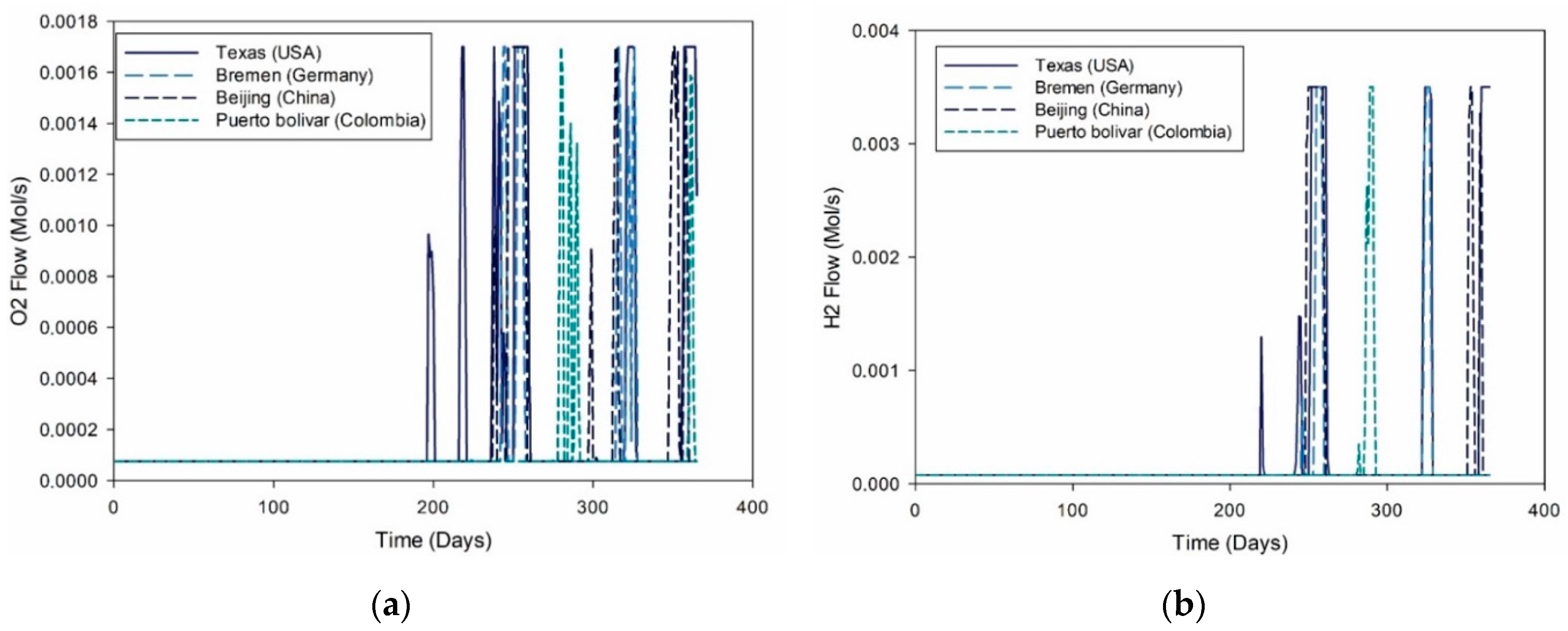
Based on the dynamic conditions established for the different places of interest by the control system, an evaluation of the behavior of the molar flows of $H_2$ and $O_2$ was carried out to identify the energy contribution of the PEM cell. The PEM cell complemented the energy generation provided by the wind turbine and the solar cell, achieving with these three, the dynamic load required by the system. The PID control system regulated this molar flow. This regulation resulted in the behavior presented in Figure 8. For the case of $O_2$ flow observed in Figure 8a, the molar flow was maintained at its minimum value to keep the PEM cell in operation without making energy contributions to the hybrid generation system in the four locations studied. On 19th October (day 292 of the year), the $O_2$ flow in Texas increased from $7.50\times {10}^{-5}$ mol/s to $5.50\times {10}^{-4}$ mol/s; this same increase was presented on 21 October (day 294 of the year) and 12 October (day 285 of the year) for Bremen and Beijing, respectively. As for Puerto Bolivar, the increase in the flow reached the value of $5.79\times {10}^{-4}$ mol/s on 11 November.

Similarly, for the flow of $H_2$ presented in Figure 8b, the molar flow was kept at its minimum value to keep the PEM cell in operation without providing energy to the hybrid generation system in the four locations studied. The increment of the molar flow of $H_2$ for 22 October went from $7.50\times {10}^{-5}$ mol/s to $2.91\times {10}^{-3}$ for Texas. Similarly, for Bremen, it went from $7.50\times {10}^{-5}$ mol/s to $8.32\times {10}^{-4}$ mol/s on 23 October, and from $7.50\times {10}^{-5}$ mol/s to $1.94\times {10}^{-3}$mol/s on 14 October for Beijing. In the case of Puerto Bolivar, on 29 November there was an increase from $7.50\times {10}^{-5}$ mol/s to $2.14\times {10}^{-3}$mol/s. The days indicated with an increment for $H_2$ and $O_2$ are the first days on which the PEM cell contributed to the generation to achieve the required load.

Two of the limitations to the proposed control system for the hybrid system based on non-conventional energy sources were to model the components of the system and to know the meteorological variables that allow for prediction of the energy generation of the system. Thus, Song-Yul Choe [41] performed dynamic modeling of a PEM-type fuel cell, where the load demand, fuel flow, and temperature play an important role when applying a control system. The dynamics and performance of the designed controllers were evaluated and analyzed by simulations using dynamic fuel cell system models, similar to the one proposed in the current study, using a multistep current and an actual load profile.

Likewise, Granda-Gutiérrez et al. [42] presented a model of a fuel cell integrated to a solar panel array and studied the effect of solar irradiation and solar cells on the voltage, current, and power of the fuel cell. One of the main limitations of that work, compared to the results presented in the current article, is that the system considers the wind resource in the hybrid system, and it also allows for the study of the time evolution of the complementarity of the energies and the performance of the control system to satisfy the energy demand.

For the case of load profile 2, Figure 9 illustrates the molar flow behavior of $H_2$ and $O_2$. Figure 9a shows the variation of $O_2$ flow required for the PEM cell. Initially, for the four locations, the flow presented is the minimum to keep the PEM cell working, and from 10th July, the $O_2$ flow for Texas showed an increase from $7.50\times {10}^{-5}$ mol/s to $9.65\times {10}^{-4}$ mol/s. Similarly, on 31 August and 4 September there was a change compared to the minimum flow value of $O_2$ in Bremen and Beijing, respectively; it went from $7.50\times {10}^{-5}$ mol/s to $1.29\times {10}^{-3}$ mol/s for Bremen and from $7.50\times {10}^{-5}$ mol/s to $1.70\times {10}^{-3}$ mol/s for Beijing. In the case of Puerto Bolivar, the increase of the minimum molar flow value of $O_2$ occurred on 7 October and went from $7.50\times {10}^{-5}$ mol/s to $1.70\times {10}^{-5}$ mol/s.

As for the flow of $H_2$, in Figure 9b it can be seen that for the case of Texas, on day 220 the first increase in molar flow was presented, going from $7.50\times {10}^{-5}$ mol/s a $1.26\times {10}^{-3}$ mol/s. In the case of Bremen and Beijing, the first increases occurred on 3 September and 6 September, respectively; going from $7.50\times {10}^{-5}$ mol/s to $7.77\times {10}^{-4}$ mol/s for the Bremen and from $7.50\times {10}^{-5}$ mol/s to $3.00\times {10}^{-3}$ mol/s for Beijing. On the other hand, in Puerto Bolivar, this increase in molar flow did not occur until 8 October, from $7.50\times {10}^{-5}$ mol/s a $1.10\times {10}^{-4}$ mol/s.

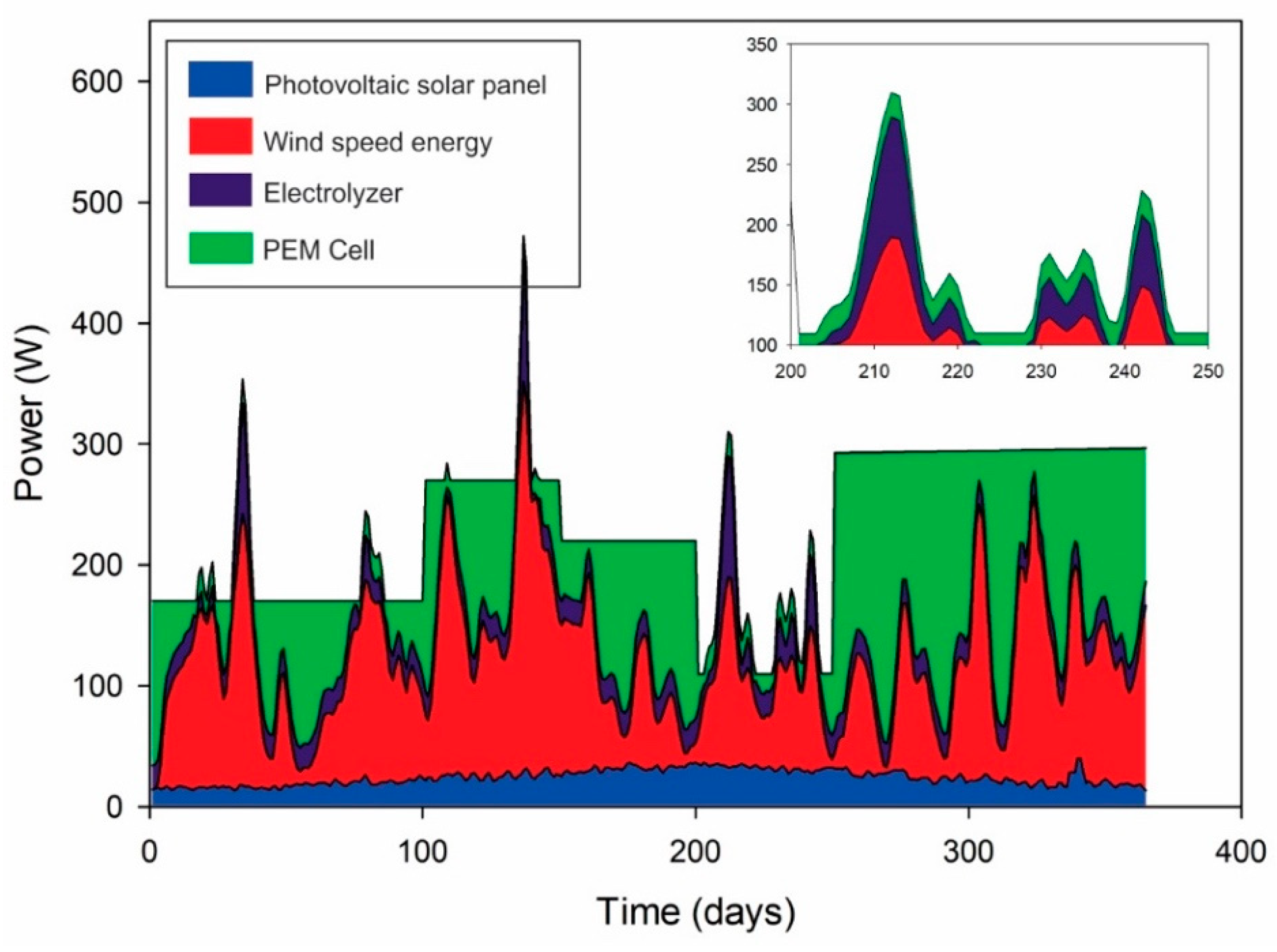
The variations in the intensities of solar radiation and wind speed that motivate these variations in the molar flows of $H_2$ and $O_2$ change the amount of power generated by each of the sources. These combinations are variable for each of the geographical areas analyzed, as well as for each load profile. These powers were analyzed for each of the areas studied. Figure 10 shows the power generated by the system for Puerto Bolivar (Colombia) for the demanded load profile 1. Figure 10 highlights what happened between 19 July and 7 September, days on which the generated power exceeded the power demand stipulated in the load profile. This was due to above-average winds and a slight increase in average solar radiation added to the low demand at this time of year, which led to the observed overshoot.

Similarly, Figure 11 shows the power generated by the system in Beijing (China) for load profile 1. As in the previous case, increases in solar radiation and wind speed and a decrease in load demand coincide. This point is relevant due to the fact that the excess in the demanded charge was maintained from 19 July to 7 September, unlike the cases that occured on the previous days, which were only daily peaks in wind speed. This figure also shows the influence of the solar radiation peak highlighted in Figure 6; this increase in radiation occurred at the time of year when the load demand for the simulation was higher, so the system needed the PEM fuel cell operation to achieve the load demand. However, the tunning parameters of the control system are responsible for ensuring that the hybrid system follows the energy demand, regardless of the wind or solar resource peaks.

Likewise, Figure 12 shows the power generated by the system in Texas (USA) for load profile 1. Figure 11 highlights the last days of January, together with the month of February, in which there was an increase in wind speed, causing a generated power higher than the demanded load profile. The rest of the time, the generation contributed by the solar radiation and the wind was complemented with the contribution of the PEM cell; this contribution is evident in the increase of the flows of $H_2$ and $O_2$ presented in Figure 8a,b.

In the case of Bremen (Germany), the results are presented in Figure 13. In Figure 13 it can be seen that in the first 100 days of the year, there were peaks in wind speed, which triggered an increase in the energy generated that exceeded the load profile. This increase was the highest presented in the four locations analyzed and is due to the increase in wind speed presented on those days, which, as in the previous peaks, generated a high activity in the electrolyzer observed in the purple area. Similarly, Figure 13 shows that the contribution of solar energy made at the peak of solar radiation highlighted in Figure 6 is not as high as the contribution made by the wind speed when it reached more than 10 m/s in the following days.

These generation peaks occur due to increased wind and solar radiation causing an overshoot of the load demanded by the profile. In

Table 6. Monthly generated renewable energy for demand 1.

		January	February	March	April	May	June	July	August	September	October	November	December
Puerto Bolivar	Solar panel (W)	1113.14	1019.97	1162.99	1157.18	1249.20	1210.05	1207.60	1226.76	1221.16	1263.60	1187.46	1218.06
	Wind power (W)	3054.36	2219.46	3075.58	3524.64	5324.62	2666.39	1831.65	2455.06	1452.63	2887.87	3807.78	3553.83
	PEM cell (W)	1042.01	1600.55	1079.52	1912.28	1751.58	2154.79	2464.76	538.48	4348.91	4337.55	3278.97	3782.90
	Total generated (W)	5209.50	4839.98	5318.09	6594.10	8325.40	6031.22	5504.01	4220.30	7022.69	8489.01	8274.20	8554.79
	Total demand (W)	4650.00	4200.00	4650.00	6500.00	7700.00	6000.00	4874.72	2783.02	6906.46	8489.01	8247.00	8554.79
	Difference (W)	559.50	639.98	668.09	94.10	625.40	31.22	629.29	1437.27	116.23	0.00	27.20	0.00
Beijing	Solar panel (W)	477.16	459.22	614.75	715.46	810.14	927.19	1033.32	977.13	866.45	727.82	602.23	645.93
	Wind power (W)	3054.36	2219.46	3075.64	3524.52	5324.69	2666.62	1831.64	2455.23	1452.48	2888.40	3807.53	3554.36
	PEM cell (W)	1385.43	2017.82	1334.14	2300.87	2057.70	2406.19	2586.94	565.96	4673.54	4872.80	3837.24	4354.50
	Total generated (W)	4916.95	4696.50	5024.53	6540.84	8192.53	6000.00	5451.90	3998.32	6992.47	8489.01	8247.00	8554.79
	Total demand (W)	4650.00	4200.00	4650.00	6500.00	7700.00	6000.00	4874.72	2783.02	6906.46	8489.01	8247.00	8554.79
	Difference (W)	266.95	496.50	374.53	40.84	492.53	0.00	577.18	1215.29	86.02	0.00	0.00	0.00
Bremen	Solar panel (W)	794.93	726.55	863.46	803.28	916.54	1003.02	1062.57	1038.76	958.51	930.13	852.45	867.23
	Wind power (W)	5531.56	4130.87	6764.05	3091.63	2538.34	2183.29	2466.17	2044.20	2414.06	3894.32	2178.62	4469.09
	PEM cell (W)	1074.83	778.89	1063.15	2605.09	4245.11	2813.69	1658.91	652.03	3752.50	3664.57	5215.94	3308.48
	Total generated (W)	7401.32	5636.32	8690.66	6500.00	7700.00	6000.00	5187.65	3734.99	7125.07	8489.01	8247.00	8644.80
	Total demand (W)	4650.00	4200.00	4650.00	6500.00	7700.00	6000.00	4874.72	2783.02	6906.46	8489.01	8247.00	8554.79
	Difference (W)	2751.32	1436.32	4040.66	0.00	0.00	0.00	312.93	951.96	218.61	0.00	0.00	90.02
Texas	Solar panel (W)	909.22	943.32	1019.30	1006.53	1179.46	1196.30	1235.67	1282.45	1186.99	1125.79	969.42	962.92
	Wind power (W)	2550.50	3006.07	2748.95	3384.86	3778.39	1827.29	1566.28	997.79	1726.32	2422.11	2320.54	2745.78
	PEM cell (W)	1528.65	549.47	1282.41	2108.60	2774.74	2976.41	2297.38	597.02	3993.14	4941.11	4957.04	4846.08
	Total generated (W)	4988.37	4498.85	5050.67	6500.00	7732.59	6000.00	5099.34	2877.26	6906.45	8489.01	8247.00	8554.79
	Total demand (W)	4650.00	4200.00	4650.00	6500.00	7700.00	6000.00	4874.72	2783.02	6906.46	8489.01	8247.00	8554.79
	Difference (W)	338.37	298.85	400.67	0.00	32.59	0.00	224.62	94.24	0.00	0.00	0.00	0.00

, a sum of the total energy generated monthly by the solar panel, the wind turbine, and the PEM cell for load profile 1 is presented. In addition, a comparison is made with the load demanded for the same period in each of the areas studied. This comparison allows us to observe that Bremen is the location with the highest excess energy generated due to the peaks of wind speed and solar radiation in the whole simulated period, reaching 9801 W, well above the 1389 W in Texas, equivalent to 14% of the excess energy generated in Bremen. Likewise, 3549 W was generated in excess in Beijing to reach 36% of what was generated in Bremen. Finally, in Puerto Bolivar, 4828 W was generated, reaching 49% of what was generated in Bremen. In spite of this, Bremen is the location with the second-highest number of months with a generation equal to the demand due to the load profile reaching 5 months, only surpassed by Texas that reached 6 months without excess generation, which shows that the high wind and solar activity presented in the first 3 months was decisive to achieve the 9801 W of excess generation in Bremen.

On the other hand,

Table 7. Monthly generated renewable energy for demand 2.

		January	February	March	April	May	June	July	August	September	October	November	December
Puerto Bolivar	Solar panel (W)	1113.14	1019.97	1162.99	1157.18	1249.20	1210.05	1207.60	1226.76	1221.16	1263.62	1187.48	1218.08
	Wind power (W)	3054.36	2219.46	3075.58	3524.64	5324.62	2666.39	1831.65	2455.06	1452.63	2888.39	3808.04	3553.93
	PEM cell (W)	1244.27	2649.25	1933.61	1548.55	1751.58	2154.79	2639.16	1294.45	4163.16	2320.30	1810.89	2864.61
	Total generated (W)	5411.76	5888.69	6172.17	6230.37	8325.40	6031.22	5678.42	4976.27	6836.95	6472.32	6806.40	7636.62
	Total demand (W)	5188.68	5516.11	5994.54	5973.29	7700.00	6000.00	5486.00	4855.37	6836.93	6268.42	6364.49	7636.61
	Difference (W)	223.08	372.58	177.63	257.08	625.40	31.22	192.42	120.90	0.02	203.90	441.92	0.02
Beijing	Solar panel (W)	477.16	459.22	614.75	715.48	810.20	927.22	1033.31	977.16	866.49	727.88	602.22	645.81
	Wind power (W)	3054.36	2219.46	3075.58	3524.64	5324.62	2666.39	1831.65	2455.06	1452.63	2887.87	3807.78	3553.83
	PEM cell (W)	1659.44	3098.64	2313.87	1914.40	2058.10	2406.39	2787.40	1528.74	4517.83	2798.72	2189.40	3436.95
	Total generated (W)	5190.96	5777.32	6004.20	6154.51	8192.92	6000.00	5652.36	4960.96	6836.95	6414.47	6599.39	7636.59
	Total demand (W)	5188.68	5516.11	5994.54	5973.29	7700.00	6000.00	5486.00	4855.37	6836.93	6268.42	6364.49	7636.61
	Difference (W)	2.28	261.21	9.66	181.22	492.92	0.00	166.37	105.59	0.02	146.05	234.90	0.01
Bremen	Solar panel (W)	794.93	726.55	863.46	803.28	916.54	1003.02	1062.57	1038.71	958.51	930.09	852.47	867.12
	Wind power (W)	5531.56	4130.87	6764.05	3091.63	2538.34	2183.29	2466.17	2044.37	2413.68	3894.36	2178.16	4469.09
	PEM cell (W)	1363.02	1583.52	1490.13	2104.98	4245.11	2813.69	1993.33	1866.19	3464.73	1600.83	3333.86	2509.48
	Total generated (W)	7689.51	6440.95	9117.64	5999.89	7700.00	6000.00	5522.08	4949.27	6836.93	6425.27	6364.49	7845.70
	Total demand (W)	5188.68	5516.11	5994.54	5973.29	7700.00	6000.00	5486.00	4855.37	6836.93	6268.42	6364.49	7636.61
	Difference (W)	2500.83	924.84	3123.10	26.60	0.00	0.00	36.08	93.91	0.00	156.85	0.00	209.09
Texas	Solar panel (W)	909.22	943.32	1019.30	1006.53	1179.46	1196.30	1235.66	1282.46	1186.98	1125.75	969.41	963.01
	Wind power (W)	2550.50	3006.07	2748.95	3384.86	3778.39	1827.29	1566.28	997.92	1726.24	2421.76	2320.64	2746.04
	PEM cell (W)	1893.94	1566.72	2269.55	1581.89	2774.74	2976.41	2684.06	2575.00	3923.68	2720.93	3074.43	3927.56
	Total generated (W)	5353.66	5516.11	6037.80	5973.29	7732.59	6000.00	5486.00	4855.37	6836.91	6268.44	6364.47	7636.60
	Total demand (W)	5188.68	5516.11	5994.54	5973.29	7700.00	6000.00	5486.00	4855.37	6836.93	6268.42	6364.49	7636.61
	Difference (W)	164.98	0.00	43.26	0.00	32.59	0.00	0.00	0.01	0.02	0.01	0.01	0.00

presents for load profile 2 the total sum of the energy generated monthly for each of the actors in the hybrid generation system. It shows Bremen as the location with the greatest excess of energy generated, reaching 7071 W, quite far from the excess generated in Texas, which only reached 204 W, meaning only 3.41% of the excess generated in Bremen. Likewise, in Beijing, 1600 W of excess energy was generated, representing 22% of the excess generated in Bremen. On the other hand, Puerto Bolivar was the closest location to Bremen, with an excess generation of 2646 W, being 37% of what Bremen generated. Besides this, Puerto Bolivar was the location that presented an excess of generation in more months, with 10 months exceeding the demand presented by the load profile 2. Only in September and December was this demand not exceeded. The opposite was the case with Texas, where the demand for the profile was exceeded in only three months and the PEM cell had to cover the demand imposed by the load profile.

For the evaluation of the performance of the controllers, the four indices selected for this evaluation are presented in Figure 14. For each of these indexes, the stabilization times were calculated, and the sum of all these times during the simulation year was plotted, obtaining two indicator values for each location studied. Figure 14a shows the IAE values for load profile 1 in black and for load profile 2 in gray; it can be seen that the stabilization time for load profile 2 is approximately 21% less on average, with the smallest time difference in Puerto Bolivar, presenting 17% less time for the second load profile. Figure 14b shows that the trend presented in the IAE is maintained in the ISE. In this indication, the stabilization time is more significant for load profile 1, and on average, the time for load profile 2 is approximately 31% less, reaching the most considerable difference in Texas where the stabilization time for the second load profile is 45% less. This significant difference in stabilization time occurs for two main reasons. The first is the difference in the load profiles; the changes in the load are smoother than in the second load profile than they are in the first. The second reason for this shorter stabilization time is that the power generated by the system in Texas for the second load profile almost never exceeds the demanded load, which allows reaching the setpoint more easily.

On the other hand, in Figure 14c the ITAE indicator is shown, in which it can be observed that, as in the two previous cases, the second load profile generates a time of stabilization less than the first, due to the smooth variation in the load demanded from the system. In this indicator, the load profile is 27% less on average for the four locations, pointing to Puerto Bolivar as the location that presented a smaller difference than the others, reaching a 19% difference between the profiles. This is due to the constant surpassing of the demanded load profile, caused by the constant increases in wind speed in this area.

Finally, Figure 14d shows, for the ITSE indicator, the most significant difference in stabilization time between the two load profiles. On average, the time for the second load profile is 44% less than the time required by the control system to achieve stabilization for the first profile. In this indicator, the difference in stabilization time between the two profiles presented in Texas is 57%. This difference is due to the fact that solar and wind power generation was always below the load profile.

The results presented in this article were developed from a dynamic hybrid system model similar to the one proposed by M.T. Iqba et al. [29], who presented the simulation of a photovoltaic component system, considering only a Southwest Wind Power Inc. AIR 403 wind turbine, a PEM fuel cell, and an electrolyzer. The dynamic model was evaluated in Simulink, and the transient responses of the system under a step change of the power load and wind speed were studied, regulating the system with a classical PID control system. In addition, G. E. Valencia et al. [43] tested the hybrid system model without a solar photovoltaic source and improved the energy performance using the generalized predictive control system, also simulated in MATLAB/Simulink software, which is a widely software used to simulate model of energy generation systems [44]. However, the application of this hybrid system guarantees the maximum use of the renewable energy resources available in the places selected in this study, since they are places with high solar radiation.

4. Conclusions

When reviewing the wind and solar behavior of the four selected locations, it was concluded that the level of solar radiation presented by Puerto Bolivar was higher than that presented by Texas, Beijing, and Bremen. Only Texas presented a similar behavior due to the fact that both regions are desert zones. As for the wind speed, the behavior presented was much more variable, with each region presenting its peak at different times of the year. The highest peaks occurred in the first three months of the year in all four locations.

Similarly, the simulation allowed us to conclude that the implementation of a PEM cell as a support to wind and solar generation system was very effective in meeting variable energy demand. The PEM cell, together with a PID system, was able to deliver the necessary energy in spite of the fact that in some seasons of the year, the climatic conditions to cover the demand were not available, as was observed in Texas for the load profile 2. This control system was strongly affected by the high peaks in the input variables over time. This can be appreciated in the first three months of the year in Bremen. The high wind supply made it difficult for the hybrid trigeneration system to maintain a stable power output by increasing the settling time, which could cause problems by exceeding the demanded load.

In addition, the evaluation of the performance of the controller through the indicators IAE, ISE, ITAE, and ITSE, showed that the PID used presented a shorter error stabilization time when the changes in the load were smoother, and the error was given by radiation levels, and wind speeds lower than necessary, forcing the PID to vary the molar flow of $H_2$ and $O_2$.

The results allow us to conclude that the difficulty of controlling a multivariable process such as a hybrid generation system is not limited only in the number of variables, but also by the interaction that exists between the subsystems (wind turbine, fuel cell, and solar photovoltaic system). The degree of interaction will determine whether the control strategy to control the process should be decentralized or centralized. Therefore, it is necessary to have interaction measures to help make such a decision, as is the case of the relative gain matrix, which is a heuristic technique without a strong theoretical basis, but rigorous connections have been established between the relative gain matrices and the stability for systems from their transfer functions. Thus, a relative gain matrix is proposed to advance in the study of the stability of multivariable control systems of hybrid energy generation processes.

In the ITSE, it was observed that the second load profile in the study generated a lower stabilization time than the first one, due to the smooth variation in the load demanded from the system. In this indicator, the load profile was 27% lower on average for the four locations, with Puerto Bolivar standing out as the location that presented the smallest difference from the others, reaching a 19% difference between the profiles due to the variability in the study period for wind and solar resources.

References

1. Yonoff, R.E.; Ochoa, G.V.; Cardenas-Escorcia, Y.; Silva-Ortega, J.I.; Meriño-Stand, L. Research trends in proton exchange membrane fuel cells during 2008–2018: A bibliometric analysis. Heliyon 2019, 5, e01724. [Google Scholar] [CrossRef] [PubMed] [Green Version]
2. Wolfram, C.; Shelef, O.; Gertler, P. How will energy demand develop in the developing world? J. Econ. Perspect. 2012, 26, 119–138. [Google Scholar] [CrossRef] [Green Version]
3. Valencia, G.; Duarte, J.; Isaza-Roldan, C. Thermoeconomic analysis of different exhaust waste-heat recovery systems for natural gas engine based on ORC. Appl. Sci. 2019, 9, 4017. [Google Scholar] [CrossRef] [Green Version]
4. Valencia, G.; Peñaloza, C.; Forero, J. Thermoeconomic optimization with PSO algorithm of waste heat recovery systems based on organic rankine cycle system for a natural gas engine. Energies 2019, 12, 4165. [Google Scholar] [CrossRef] [Green Version]
5. Alibaba, M.; Pourdarbani, R.; Hasan, M.; Manesh, K.; Valencia, G.; Duarte, J. Thermodynamic, exergo-economic and exergo-environmental analysis of hybrid geothermal-solar power plant based on ORC cycle using emergy concept. Heliyon 2020, 6, e03758. [Google Scholar] [CrossRef]
6. Goldemberg, J. The case for renewable energies. In Renewable Energy; Routledge: Thames, UK, 2012; pp. 31–42. [Google Scholar]
7. Duarte, J.; Duarte Forero, N.; Hernandez, B.; Vanegas, M.; Stand, R. Experimental study of partial fuel substitution with hydroxy and energy recovery in low displacement compression ignition engines. In ASME International Mechanical Engineering Congress and Exposition; American Society of Mechanical Engineers: New York, NY, USA, 2019; Volume 59452, p. V008T09A021. [Google Scholar]
8. Hache, E.; Palle, A. Renewable energy source integration into power networks, research trends and policy implications: A bibliometric and research actors survey analysis. Energy Policy 2019, 124, 23–35. [Google Scholar] [CrossRef]
9. De Paulo, A.F.; Porto, G.S. Solar energy technologies and open innovation: A study based on bibliometric and social network analysis. Energy Policy 2017, 108, 228–238. [Google Scholar] [CrossRef]
10. Koo, Y.; Oh, M.; Kim, S.-M.; Park, H.-D. Estimation and mapping of solar irradiance for korea by using COMS MI satellite images and an artificial neural network model. Energies 2020, 13, 301. [Google Scholar] [CrossRef] [Green Version]
11. Alghamdi, A.S. Potential for rooftop-mounted pv power generation to meet domestic electrical demand in saudi arabia: Case Study of a villa in jeddah. Energies 2019, 12, 4411. [Google Scholar] [CrossRef] [Green Version]
12. Mao, G.; Liu, X.; Du, H.; Zuo, J.; Wang, L. Way forward for alternative energy research: A bibliometric analysis during 1994–2013. Renew. Sustain. Energy Rev. 2015, 48, 276–286. [Google Scholar] [CrossRef]
13. Yue, C.-D.; Chiu, Y.-S.; Tu, C.-C.; Lin, T.-H. Evaluation of an offshore wind farm by using data from the weather station, floating LiDAR, mast, and MERRA. Energies 2020, 13, 185. [Google Scholar] [CrossRef] [Green Version]
14. Perea-Moreno, A.-J.; Alcalá, G.; Hernandez-Escobedo, Q. Seasonal wind energy characterization in the gulf of mexico. Energies 2019, 13, 93. [Google Scholar] [CrossRef] [Green Version]
15. KC, A.; Whale, J.; Urmee, T. Urban wind conditions and small wind turbines in the built environment: A review. Renew. Energy 2019, 131, 268–283. [Google Scholar] [CrossRef]
16. Pinheiro, E.; Bandeiras, F.; Gomes, M.; Coelho, P.; Fernandes, J. Performance analysis of wind generators and PV systems in industrial small-scale applications. Renew. Sustain. Energy Rev. 2019, 110, 392–401. [Google Scholar] [CrossRef]
17. Tsay, M.-Y. A bibliometric analysis of hydrogen energy literature, 1965–2005. Scientometrics 2008, 75, 421–438. [Google Scholar] [CrossRef]
18. He, M.; Zhang, Y.; Gong, L.; Zhou, Y.; Song, X.; Zhu, W.; Zhang, M.; Zhang, Z. Bibliometrical analysis of hydrogen storage. Int. J. Hydrogen Energy 2019, 44, 28206–28226. [Google Scholar] [CrossRef]
19. Tanç, B.; Arat, H.T.; Conker, Ç.; Baltacioğlu, E.; Aydin, K. Energy distribution analyses of an additional traction battery on hydrogen fuel cell hybrid electric vehicle. Int. J. Hydrogen Energy 2019. [Google Scholar] [CrossRef]
20. Prashanth, B.N.; Pramod, R.; Kumar, G.B.V. Design and development of hybrid wind and solar energy system for power generation. Mater. Today Proc. 2018, 5, 11415–11422. [Google Scholar] [CrossRef]
21. Haddad, A.; Ramadan, M.; Khaled, M.; Ramadan, H.S.; Becherif, M. Triple hybrid system coupling fuel cell with wind turbine and thermal solar system. Int. J. Hydrogen Energy 2019, 45, 11484–11491. [Google Scholar] [CrossRef]
22. Zhang, W.; Maleki, A.; Rosen, M.A.; Liu, J. Sizing a stand-alone solar-wind-hydrogen energy system using weather forecasting and a hybrid search optimization algorithm. Energy Convers. Manag. 2019, 180, 609–621. [Google Scholar] [CrossRef]
23. Ishaq, H.; Dincer, I.; Naterer, G.F. Development and assessment of a solar, wind and hydrogen hybrid trigeneration system. Int. J. Hydrogen Energy 2018, 43, 23148–23160. [Google Scholar] [CrossRef]
24. Elliott, D.; Schwartz, M.; Haymes, S.; Heimiller, D.; Scott, G.; Flowers, L.; Brower, M.; Hale, E.; Phelps, B. 80 and 100 Meter Wind Energy Resource Potential for the United States; Windpower 2010; National Renewable Energy Lab. (NREL): Golden, CO, USA, 2010. [Google Scholar]
25. Lütkehus, I.; Salecker, H.; Umweltbundesamt, D.E. Onshore wind energy potential in Germany. DEWI Mag. 2013, 43, 23–28. [Google Scholar]
26. Liu, F.; Sun, F.; Liu, W.; Wang, T.; Wang, H.; Wang, X.; Lim, W.H. On wind speed pattern and energy potential in China. Appl. Energy 2019, 236, 867–876. [Google Scholar] [CrossRef]
27. Antonio, F.; Barrozo, F.; Valencia, G.; Obregon, L.; Arango-Manrique, A.; Núñez Alvarez, J. Energy, economic, and environmental evaluation of a proposed solar-wind power on-grid system using HOMER Pro®: A case study in Colombia. Energies 2020, 13, 761307. [Google Scholar]
28. Pandiarajan, N.; Muthu, R. Mathematical modeling of photovoltaic module with Simulink. In Proceedings of the 1st International Conference on Electrical Energy Systems (ICEES), Newport Beach, CA, USA, 3–5 January 2011; pp. 258–263. [Google Scholar]
29. Khan, M.J.; Iqbal, M.T. Dynamic modeling and simulation of a small wind–fuel cell hybrid energy system. Renew. Energy 2005, 30, 421–439. [Google Scholar] [CrossRef]
30. Şen, S.; Demirer, G. Anaerobic treatment of real textile wastewater with a fluidized bed reactor. Water Res. 2003, 37, 1868–1878. [Google Scholar]
31. Kader, A.A.; Colina-Irezabal, M.L. Métodos de mezclado, muestreo y análisis de gases. Tecnología Postcosecha de Cultivos Hortofrutícolas 2007, 24, 169–174. [Google Scholar]
32. Valencia, G.; Benavides, A.; Cárdenas, Y. Economic and environmental multiobjective optimization of a wind-solar-fuel cell hybrid energy system in the Colombian Caribbean region. Energies 2019, 12, 2119. [Google Scholar] [CrossRef] [Green Version]
33. Meshram, P.M.; Kanojiya, R.G. Tuning of PID controller using ziegler-nichols method for speed control of DC motor. In Proceedings of the IEEE International Conference on Advances in Engineering, Science and Management (ICAESM), Nagapattinam, India, 30–31 March 2012; pp. 117–122. [Google Scholar]
34. Smith, C.A.; Corripio, A.B. Principles and Practice of Automatic Process Control; Wiley: New York, NY, USA, 1985; Volume 2. [Google Scholar]
35. Shinskey, F.G. Feedback Controllers for the Process Industries; McGraw-Hill: New York, NY, USA, 1994. [Google Scholar]
36. Dorf, R.C.; Bishop, R.H. Modern Control Systems, 12th ed.; Pearson Education, Inc.: Upper Saddle River, NJ, USA, 2011. [Google Scholar]
37. Valencia Ochoa, G.; Núñez Alvarez, J.; Vanegas Chamorro, M. Data set on wind speed, wind direction and wind probability distributions in Puerto Bolivar—Colombia. Data Brief 2019, 27, 104753. [Google Scholar] [CrossRef]
38. De la Cruz Buelvas, J.; Valencia Ochoa, G.; Vanegas Chamorro, M. Estudio estadístico de la velocidad y la dirección del viento en los departamentos de Atlántico y Bolívar en Colombia. Ingeniare Revista Chilena de Ingeniería 2018, 26, 319–328. [Google Scholar] [CrossRef] [Green Version]
39. Carta, J.A.; Ramírez, P. Analysis of two-component mixture Weibull statistics for estimation of wind speed distributions. Renew. Energy 2007, 32, 518–531. [Google Scholar] [CrossRef]
40. Seguro, J.V.; Lambert, T.W. Modern estimation of the parameters of the Weibull wind speed distribution for wind energy analysis. J. Wind Eng. Ind. Aerodyn. 2000, 85, 75–84. [Google Scholar] [CrossRef]
41. He, J.; Choe, S.-Y.; Hong, C.-O. Analysis and control of a hybrid fuel delivery system for a polymer electrolyte membrane fuel cell. J. Power Sources 2008, 185, 973–984. [Google Scholar] [CrossRef]
42. Granda-Gutiérrez, E.E.; Orta, O.A.; Díaz-Guillén, J.C.; Jimenez, M.A.; Osorio, M.; Gonzleáz, M.A. Modelado y simulación de celdas y paneles solares. Congreso Internacional de Ingeniería Electrónica 2013, 35, 17–22. [Google Scholar]
43. Valencia, G.; Glen, G.; Turizo, J.; Chamorro Coneo, R.J. Mimo generalized predictive control for a small wind turbine–fuel cell hybrid energy system. In Proceedings of the ASME 2009 3rd International Conference on Energy Sustainability collocated with the Heat Transfer and InterPACK09 Conferences, San Francisco, CA, USA, 19–23 July 2009; pp. 557–562. [Google Scholar]
44. Ochoa, G.V.; Isaza-Roldan, C.; Forero, J.D. A phenomenological base semi-physical thermodynamic model for the cylinder and exhaust manifold of a natural gas 2-megawatt four-stroke internal combustion engine. Heliyon 2019, 5, e02700. [Google Scholar] [CrossRef] [PubMed] [Green Version]
Figure 1. The geographical location of the studied regions.
Applsci 10 03093 g001
Figure 2. Schematic layout of the hybrid energy generation system.
Applsci 10 03093 g002
Figure 3. Wind turbine transient response curve.
Applsci 10 03093 g003
Figure 4. Frequency distribution of wind speed for each location.
Applsci 10 03093 g004
Figure 5. Wind speeds for each location.
Applsci 10 03093 g005
Figure 6. Solar radiation for each location.
Applsci 10 03093 g006
Figure 7. The proposed syystem charge profiles.
Applsci 10 03093 g007
Figure 8. Flow for charge profile 1 for (a) O2 and (b) H2.
Applsci 10 03093 g008
Figure 9. Flow for charge profile 2 for (a) O2 and (b) H2.
Applsci 10 03093 g009
Figure 10. Power in Puerto Bolivar (Colombia).
Applsci 10 03093 g010
Figure 11. Power in Beijing (China).
Applsci 10 03093 g011
Figure 12. Power in Texas (USA).
Applsci 10 03093 g012
Figure 13. Power in Bremen (Germany).
Applsci 10 03093 g013
Figure 14. Performance indicators (a) absolute value of the error (IAE), (b) integral of the square of the error (ISE), (c) the integral of the absolute value of the error for time (ITAE), and (d) integral of the square of the error for time (ITSE).
Applsci 10 03093 g014