Classical Music Prediction and Composition by Means of Variational Autoencoders

Abstract

This paper proposes a new model for music prediction based on Variational Autoencoders (VAEs). In this work, VAEs are used in a novel way to address two different issues: music representation into the latent space, and using this representation to make predictions of the future note events of the musical piece. This approach was trained with different songs of Handel. As a result, the system can represent the music in the latent space, and make accurate predictions. Therefore, the system can be used to compose new music either from an existing piece or from a random starting point. An additional feature of this system is that a small dataset was used for training. However, results show that the system is able to return accurate representations and predictions on unseen data.

1. Introduction

Since Pythagoras, mankind has always tried to use formal instructions and processes to create or analyze music. This is not limited to the music, researchers from all times have tried to understand the laws behind a creative mind in any kind of art. Although researchers have been able to unveil some of those rules, the idea, as Turing express himself in 1950 [1], of an artificial artist continues to be a challenge, even today.

In this sense, as in many other knowledge fields, the breakthrough of Deep Learning has become an absolute revolution for art generation in recent times. Proof of that is the increasing number of advances published every year which relates art generation and Deep Learning. However, it may be highlighted that the generation of images is the one that has attracted most of the attention [2], even though other areas such as text generation have experienced also much research [3].

Focusing the attention on the combination of music processing and Deep Learning, some approaches that allow the generation of audio have arisen in recent years. However, the most used methods (Generative Adversarial Networks, GANs, and Linear Shot-Term Memories, LSTMs), are not very suitable because they are usually too complex methods and require large training datasets with long training periods [4,5].

Alternatively, there are other models for this task, such as Variational Autoencoders (VAEs) [6]. This approach combines an encoder and a decoder in order to make a transformation from a usually high-dimensional space into a lower-dimensional space. The resulting new space, called latent space, is usually more compact and keep the spatial relationship between pattern from the original space. Therefore, any latent vector between two (or more) musical pieces will return a musical piece with the properties of those mixed. This allows the user to change the values of the latent vector in order to get a similar musical piece. This feature can make VAEs a powerful technique for music composition, in which the user has more control and can change at any moment the melody being composed by the system.

VAEs have already been explored as systems for musical analysis [7]; however, its use for composition and prediction is still unexplored. This paper shows how VAEs can be used for music prediction and, therefore, for music composition from a small dataset. In this work, classical music was used for training the system and, as a result, the system is able to compose melodies similar to those of the dataset used for training. Moreover, and oppositely with other systems, VAEs allow the training with a relatively small dataset. Results show that the system is able to perform on unseen data with the same accuracy as with data used in the training process. Therefore, no large datasets are needed to develop this system and to learn from an author.

It may be highlighted that the application of the VAEs in this work differs significantly from other previous works. Usually, inputs and targets have the same value and thus VAEs are used to perform encoding-decoding operations. In the present work, a different approach is carried out. In this approach, the target values used are not identical to the inputs. Instead of it, they represent the future values of the musical piece. With this scheme, the VAE performs codification-prediction operations instead of codification-prediction operations. Therefore, the main contribution of this work is the use of VAEs to predict future parts of a musical piece.

The rest of the paper is organised as follows: Section 2 contains a description of the most relevant works in this area. Section 3 provides a description of VAEs. Section 4 describes the method used in this work, with the descripction of the representation of the music in Section 4.1, the implementation of the VAE in Section 4.2, and the different metrics used for measuring the results in Section 4.3. Section 5 describes the experiments carried out in this work. Finally, Section 6 and Section 7 describe the main conclusions of this work and the future works that can be carried out from it.

2. State of the Art

Music generation by means of Artificial Intelligence techniques is a long-time pursued objective. Although over the years several works, such as [8,9,10,11,12], have been published about music composition, one of the most used techniques in the close past for this task has been the Deep Learning approaches. As new Deep Learning models have been developed, these models have been applied to music generation because they allow new ways to process the signals.

Among the Deep Learning approches for art generation, Generative Adversarial Networks is probably the most prominent one. The technique is based on the development of two different neural networks called generator and discriminator. The generator is used to produce new plausible examples from the problem domain, while the discriminator is used to classify examples as real or fake. Although this approach has been mainly applied in image generation [13], there are some works in the field of music generation with some modifications to model the temporal structure and the multi-track interdependency of a song [4,14,15]. However, the technique is based on reaching the Nash equilibrium [16] between the generator and the discriminator which is not always easy resulting in monotonous pieces or without temporal coherence with the previous part of the piece.

Pursuing that temporal line, Convolutional Neural Networks have been used to extract features. However, its main goal was not to compose music, but to perform audio-to-MIDI alignment, audio-to-audio alignment, and singing voice separation [17]. Alternatively, other works focused their attention on the application of Long Short-Term Memory (LSTM) networks, which are networks with recurrent connections broadly used for temporal processing [18]. For example, simple LSTMs were used for musical transduction [5] to implement a pitch detection system and LSTMs were also used by [19] to model text representations of music, which uses over 2000 chord progressions for training an LSTM. However, focusing on music generation, LSTMs were combined with VAEs for music generation [20,21]. The idea behind this work was trying to keep the temporal coherence by means of the LSTM, while reducing the search space with the VAEs. The result was a two-layer LSTMs network with 1024 neurons per layer used as the decoder. The main problem is that the size of the network requires large datasets to be trained. For example, in one of the most important works with LSTMs, 23,000 music transcriptions were used to train an LSTM to create music transcription models in folk tunes [22,23]. This is probably one of the biggest musical dataset used to train a neural network model. As a result, the folk-RNN model was evaluated by a community of composers with good reviews. Deep recurrent neural networks were also used for encoding the music sequences of over 2000 tunes [24] or Bach’s compositions were used to train an LSTM for music composition [25]. However, the same approach can not be followed in most of the cases because Batch was one of the most prolific compositors, most of the datasets for a specific style/composer will be very limited in size.

Consequently, in models with fewer examples, reducing the dimensionality of the input space to is a task that some authors have tackle with Autoencoders (AEs) like [26] which used them to synthesize musical notes. Thus, the focus of this work was not to generate music compositions but independent raw musical notes. Alternatively, going along the same line, VAEs have also been used for music-based tasks [27,28]. For instance, in [7,29], VAEs were used for timbre studies. In this work, the Short-Term Fourier Transform (STFT) in combination with a Discrete Cosine Transform (DCT) and the Non-Stationary Gabor Transform (NSGT) to preprocess the audio before the application of the VAE. In another work, recurrent VAEs were used for lead sheet generation, together with a convolutional generative adversarial network for arrangement generation [30]. Those works support the fact that VAEs are a suitable approach to analyze and reduce the dimensionality with fewer examples.

Supporting this idea of the capabilities for sound analysis of the VAEs, they have been also applied to process speech signals with the objective of making modifications in some attributes of the speakers [31,32]. In another work, VAEs were combined with LSTMs used as encoders, and recurrent neural networks (RNNs) as decoders [20] and they were also used for sound modeling [33]. However, those works with raw audio instead of MIDI files since its objective is to model sound and not music generation.

Alternatively, other works have explored the improvement in VAEs by perturbing the representations in the latent space with Perlin Noise [34]. In a different work, another variation called Convolutional Variational Recurrent Neural Network that combines different neural network models is used for music generation [35], using a sequence-to-sequence model.

In this work, VAEs are going to be used in order to keep the coherence of the latent space and produce suitable outputs in music generation. Oppositely to other works, this one is going to use a small dataset of MIDI files from a single compositor. The challenge of this approach is having very small data to identify the features while using a discrete format like MIDI instead of raw or analog signals.

3. Variational Autoencoders

Variational Autoencoders arose from the evolution of autoencoders [6,36,37]. Both techniques aim to codify a set of data into a smaller vector, and then reconstructing the original data from this vector. In AEs, the set of data points in the input space is mapped to a smaller vector, which is a point in a new space with fewer dimensions called latent space. Usually, Multilayer Perceptrons (MLPs) are used for the codification and decodification tasks. This approach allows for interesting tasks such as information compression. However, in this latent space, other points different than those obtained from an input do not usually correspond to output with significance in the original space.

The latent space built by VAEs is usually more compact by the other latent spaces built by other techniques such as autoencoders. Thus, in this latent space, those similar inputs usually have latent representations close to each other, and the points in the space between them correspond to outputs that have a significance in the original space. VAEs allow powerful representations while being a simple and fast learning framework.

The objective of Variational Autoencoders is to find the underlying probability distribution of the data $p\left(x\right)$, where x is a vector in a high dimensional space. In a lower-dimensional space z, a set of latent variables are considered. It should be noticed that, on the following equations, the bold font variables always represent vectors while regular ones represent single values. The model is defined by the probability distribution described in the Equation (1).

$$p(\mathbf{x},\mathbf{z})=p\left(\mathbf{x}\right|\mathbf{z}\left)p\right(\mathbf{z}).$$

(1)

The function $p\left(\mathbf{x}\right|\mathbf{z})$ represents a probabilistic decoder that models how the generation of observed data $\mathbf{x}$ is conditioned on the latent vector $\mathbf{z}\sim p\left(\mathbf{z}\right)$, i.e., describes the distribution of the encoded variable given the original one. The function $p\left(\mathbf{z}\right)$ represents the probability distribution of the latent space and is usually modeled by a standard Gaussian distribution. For a specific observation $\mathbf{x}$, the latent vector can be calculated as $\mathbf{z}\sim p\left(\mathbf{z}\right)$, and from this vector an approximation of the original input vector can be calculated by $\mathbf{x}\sim p\left(\mathbf{x}\right|\mathbf{z})$.

The probabilistic encoder is given by the function $p\left(\mathbf{z}\right|\mathbf{x})$, which describes the distribution of the encoded variable given the original one. Given the Bayesian rule (Equation (2))

$$p\left(\mathbf{z}\right|\mathbf{x})=\frac{p\left(\mathbf{x}\right|\mathbf{z}\left)p\right(\mathbf{z})}{p\left(\mathbf{x}\right)}=\frac{p\left(\mathbf{x}\right|\mathbf{z}\left)p\right(\mathbf{z})}{\int p\left(\mathbf{x}\right|\mathbf{z}\left)p\right(\mathbf{z})dz}.$$

(2)

The integral in the denominator can be approximated by means of variational inference with distribution $q\left(\mathbf{z}\right|\mathbf{x})$. This model works as an encoder, and, for a specific $\mathbf{x}$, emits two latent vectors, $\mathbf{\mu }$ and $\mathbf{\sigma }$, that represent the mean and standard deviation of the Gaussian probability for that data:

$$q\left(\mathbf{z}\right|\mathbf{x})=\mathcal{N}(\mathbf{z};\mathbf{\mu }\left(\mathbf{x}\right),{\mathbf{\sigma }}^2\left(\mathbf{x}\right)).$$

(3)

The optimization problem consists of minimizing the Kullback–Leibler (KL) divergence between the approximation and the original density. This value measures the information lost when using $q\left(\mathbf{z}\right|\mathbf{x})$ to approximate $p\left(\mathbf{z}\right|\mathbf{x})$, and is given by:

$$D_{KL}\left(q\left(\mathbf{z}\right|\mathbf{x})\right|\left|p\left(\mathbf{z}\right|\mathbf{x})\right)={\mathbb{E}}_{q\left(\mathbf{z}\right)}\left[logq\left(\mathbf{z}\right|\mathbf{x})\right]-{\mathbb{E}}_{q\left(\mathbf{z}\right)}\left[logp(\mathbf{x},\mathbf{z})\right]+logp\left(\mathbf{x}\right).$$

(4)

This equation can be rewritten as

$$logp\left(\mathbf{x}\right)=D_{KL}\left(q\left(\mathbf{z}\right|\mathbf{x})\right|\left|p\left(\mathbf{z}\right|\mathbf{x})\right)-{\mathbb{E}}_{q\left(\mathbf{z}\right)}\left[logq\left(\mathbf{z}\right|\mathbf{x})\right]+{\mathbb{E}}_{q\left(\mathbf{z}\right)}\left[logp(\mathbf{x},\mathbf{z})\right].$$

(5)

Here, a function called evidence lower bound (ELBO) can be defined. This value allows the calculation of the approximate posterior inference. Given that $\varphi$ denotes the parameters of the encoder and $\theta$ the parameters of the decoder (weights and biases), the ELBO function can be written as:

$$ELBO(\varphi ,\theta ,\mathbf{x})={\mathbb{E}}_{q\left(\mathbf{z}\right)}\left[logp(\mathbf{x},\mathbf{z})\right]-{\mathbb{E}}_{q\left(\mathbf{z}\right)}\left[logq\left(\mathbf{z}\right|\mathbf{x})\right].$$

(6)

Therefore Equation (5) can be rewritten as:

$$logp\left(\mathbf{x}\right)=D_{KL}\left(q\left(\mathbf{z}\right|\mathbf{x})\right|\left|p\left(\mathbf{z}\right|\mathbf{x})\right)+ELBO(\varphi ,\theta ,\mathbf{x}).$$

(7)

Since the KL divergence is greater than or equal to zero, minimizing this KL divergence is equivalent to maximizing the ELBO function. Therefore, the objective can be changed into maximizing the marginal log-likelihood $log{p}_{\theta }\left(\mathbf{x}\right)$ over a training dataset of vectors $\mathbf{x}$. In order to accomplish maximize the ELBO function, a stochastic gradient descent process is performed to optimize the parameters (weights and biases).

Many times a $\beta$ value is introduced in the second term, leading to the $\beta$-VAE formulation. In this formulation, a Lagrangian multiplier $\beta$ is introduced, and together with the application of the Karush-Kuhn-Tucker conditions, allow to weight the relative importance of the reconstruction error with the compactness of the latent space. A compact latent space usually leads to having more interpretable decodification vectors.

The parameter $\beta$ controls the influence of the second objective: higher values of this parameter give more importance to the statistical independence than on the reconstruction, making the decodification of latent vectors more interpretable. However, this also has a drawback: less importance is given to the reconstruction error. With a value of $\beta =1$, then the model will be identical to a VAE. This modification can lead to having better results [6]; however, some works suggest a modification of this parameter through the training process [37]. This term allows the control of the trade-off between output signal quality and compactness/orthogonality of the latent coefficients $\mathbf{z}$.

4. Model

4.1. Representation

The model proposed in this paper uses a representation of the music with the shape of a binary matrix M with dimensions $n\times t$, where n is the number of pitches and t is time. In this work, a time step of 100 milliseconds was used. This period was used because it was found that the reconstruction of the songs with it resulted in very low differences with the original ones. Therefore, $M_{ij}=1$ for those moments j in which a pitch i is being played, while $M_{ij}=0$ when that pitch is not being played. In this codification, the velocity (i.e., the volume) of the note events has not been taken into consideration.

This matrix was built from an MIDI file that contains the notes and their durations. In this case, the used MIDI files are in physical time. From these files, the notes were read and the matrix M was built. A note with a pitch i that begins in the instant t and has a duration of $100*d$ milliseconds was situated in row i, and in the columns from t to $t+d$. In the case of having two consecutive overlapping notes with the same pitch, the matrix M had, on that note, a series of 1 s from the beginning of the first note to the end of the second, with no distinction of being one long note or two different overlapping notes. To make this distinction, the value of M at the moment previous to the second note was set to 0.

To make the dataset, 14 different compositions of Handel were used. Although it may seem a very low number, one of the objectives of this work is to show that this system can learn the representation of the latent space with a small dataset, and the resulting model can learn correctly from an author.

Table 1. Information about the compositions used in this work.

Name	Duration
Aylesford Air	2:51
Aylesford Fughette	0:54
Aylesford Gavotte	1:32
Aylesford Menuet in Am	2:59
Aylesford Menuet in D	2:33
Aylesford Passepied	0:53
Aylesford Sarabande	3:01
Aylesford Sonata	3:52
Gigue in G	2:07
Harmonious Blacksmith Op107	7:01
Hirtensinfonie	2:37
Joy to the World	1:14
Overture from the Messiah	3:22
Courante from Suite No. 11	2:42

shows a summary of the compositions used in this work. Each composition was extracted from a different MIDI file and codified into binary matrices as described above. The midi files were downloaded from https://www.classicalguitarmidi.com/.

4.2. Autoencoder Implementation

Once the matrices were obtained, the inputs and targets of the VAE were elaborated. In a traditional approximation, the inputs and targets of the VAE were the same vectors. However, in this particular case, a different approach was used. The inputs were a time window of T seconds of the matrix M, i.e., a set of consecutive columns reshaped as a vector. An overlapping of $T-1$ seconds was used for building different inputs from the same matrix. In this case, the targets for these inputs were not the same vector. Instead of it, the target for each input was the following input assuming a Markov chain. Since an input and the following one had a difference of 1 s, $T-1$ seconds of the targets correspond to values in the inputs, and 1 s of the targets are new musical notes.

With this approach, we want the VAE not only to learn the dependencies between notes that allow making a representation in the latent space, but also the dependencies with the next second of music. Therefore, VAE is aimed to solve two different problems: music recomposition and music prediction. Once T seconds of music are codified into a latent vector, the decodification of this vector returns the following T notes with overlapping of $T-1$ seconds. Therefore, with this VAE trained, the generation of new musical compositions is very simple. First, T initial seconds of music are taken. These seconds may be some already existing seconds from any composition or the decodification of any random vector in the latent space. Then, these seconds are used as inputs to the VAE to generate T seconds in which the first $T-1$ are overlapping. Thus, 1 second of new music is generated. These T seconds can be used again as inputs to generate a new second, and therefore a loop is built in which it can have as many iterations as seconds are needed.

It is important to bear in mind that this system cannot be used to fill a gap in a composition, but to continue an unfinished composition. If the system is used for this purpose, then the T initial seconds will be an existing part of the composition, and the system will try to continue this composition in the same way as Handel would have done.

Moreover, the part given by the system is not unique. Different parts can be returned if the vector is modified in the latent space. In this sense, this system allows the composition of different continuations.

Since a VAE is used, a loss function has to be given. This loss function was defined in Section 3. In this implementation, sigmoid functions are used in the output layer, and therefore the system returns values between 0 and 1. In order to build music representation as a boolean matrix as described in Section 4.1, a threshold must be used. This threshold is used for obtaining the matrix that represents a MIDI from the outputs of the neural network. This threshold is used for obtaining the matrix that represents a MIDI from the outputs of the neural network by converting the numerical output values of the ANN to boolean values. The transfer function used in the output layer is sigmoid, so the outputs are in the rank from 0 to 1. Therefore, an output value higher than the threshold means the presence of a pitch in that timestep, and a lower value means the absence of a pitch in that timestep. As a consequence, the threshold value allows us to convert a numeric matrix into a boolean matrix that represents the musical information. Experimentation with different thresholds has to be done in order to find one the returns the best results. Low values will make the system return musical pieces with many pitches, while high values will make the system return musical pieces with less pieces.

During the training process, in each step, the inputs used were the ground truth, not the generated ones. However, the system can be run using the generated outputs as new inputs to the system.

4.3. Performance Measures

In order to measure the behavior of this system, the outputs generated by this system, after the application of the threshold, must be compared with the targets. Since both outputs and targets are boolean values, this comparison can be done by means of Accuracy (ACC), Sensitivity (SEN) and Predictive Positive Value (VPP).

These values can be calculated from a confusion matrix. This matrix is built from four values:

• True Positives (TP) is the number of pitches and time steps correctly played.
• False Positives (FP) is the number of pitches played in a time step in which there should be silence.
• True Negatives (TN) is the number of pitches and time steps in which no notes are played and there should be silence.
• False Negatives (FN) is the number of pitches and time steps in which no notes are played but there should be played.

From these values, ACC, SEN and VPP can be calculated with the following equations [38]:

$$ACC=\frac{TP+FP}{TP+FP+TN+FN}$$

(8)

$$SEN=\frac{TP}{TP+FN}$$

(9)

$$VPP=\frac{TP}{TP+FP}.$$

(10)

ACC represents the ability of the model to play values adequately. SEN represents the ability to play the true notes, even some additional notes might be played. PPV is the probability of the system that the notes played correspond to true notes, even if some true notes are left to be played.

Since SEN and PPV are important measures, a good trade-off between SEN and PPV is needed. These values, as well as ACC, highly depend on the threshold chosen. A low value on the threshold leads to having a high number of notes played, even if many of them do not correspond to the original piece. A high value of the threshold corresponds to having a low number of notes, but with a high probability that they belong to the original piece.

Many times, these two measures (SEN, PPV) are summarized in a single metric called the F1 score. This metric is with the harmonic mean of SEN and PPV metrics and it is usually better than accuracy on imbalanced binary data, as is the case of this dataset [39].

5. Experiments

In order to develop the system described in Section 4.2, different experiments were carried out to set the values of the different parameters.

As it was already said, the system tries to predict 1 s of music from $T-1$ seconds of music. Therefore, this value of T is an important parameter. Low values doe not give enough information to predict the music. On the other hand, too large values may give too much information and make the training process too slow, and overfit to the training set. The experimentation was performed with values of $T=2$ to $T=10$ s. These values of window length were the results of some preliminary experiments using different values for T. Additionally, a value of $T=1$ was also chosen, in order to make predictions of 0.5 s instead of 1 s. These windows were overlapping, so very little information on the ending of pieces had to be discarded.

With respect to the architecture of the network, in all of the cases, the decoder was an MLP with one hidden layer and the decoder had the same architecture. An important parameter is the number of neurons in the hidden layers. Experiments with 500 and 750 neurons were performed. These values were chosen to be very different to study the impact of this hyperparameter.

Another important parameter was the dimension of the latent space. In this sense, values of 100 and 200 were chosen for this parameter. As with the number of neurons, very different values of this hyperparameter were chosen to study its impact. Finally, a value of $\beta =0.5$ was used in these experiments, as described in Section 3.

The dataset was randomly divided leaving different compositions in the training and test sets. The idea of this division is to test the system in some compositions different than the ones used in training so the measurements in the test set are completely independent of those of the training set. Since 14 compositions were used, 78.57% of the compositions were for training and 21.43% were used for test, i.e., 11 compositions were used for training and 3 were used for test. An ADAM optimizer was used with a learning rate of 0.001.

The system was trained with all of the parameter configurations described. For each configuration, different thresholds were used in order to select the best threshold and configurations. Figure 1 shows the results obtained for each configuration. The figures on the left show the F1 scores and accuracies obtained with the best threshold for each configuration on the training set. The figures on the right show the F1 scores and accuracies obtained on the test set with the thresholds given by the left figures. As can be seen, accuracies and F1 scores are very high on both training and test sets. Moreover, having a larger number of neurons (750) seems to return much better results than with a lower number (500). When using a specific number of hidden neurons, whether it is 500 or 750, a different latent dimension does not seem to return very different results. A higher latent dimension seems to return slightly higher results; however, the difference was very low. Therefore, the number of neurons seems to be a hyperparameter with a higher impact on the system. From this figure, a configuration with a window size of 9 seg, 750 hidden neurons and a latent dimension of 200 was chosen since it returned the best results on the training dataset.

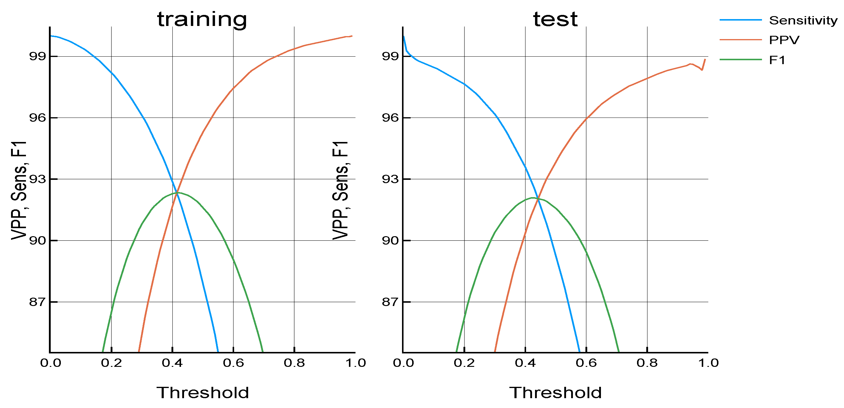
Figure 2 shows the results obtained with a different threshold for this configuration. This figure shows Sensitivity, PPV and F1 score on training and test sets. As was explained, low threshold values lead to having compositions with more notes, while high values lead to having fewer notes. Therefore, low threshold values lead to having high sensitivity and low PPV. On the other side, a high threshold leads to having low sensitivity and high PPV. Therefore, a trade-off between these two values is needed. For this reason, the F1 score was used. As a result, the value with the highest F1 score in the training set was used as a threshold, being this value 0.41. The right plot shows the sensitivity, PPV and F1 score for the test set.

All of these performance values were calculated as a result of the training process. As Figure 1 and Figure 2 show, results in the test sets are slightly worse than in the training set. This means that the codification and decodification performed by the system on unseen data (i.e., different musical pieces) are almost as accurate as on the data used for training.

As these figures show, the train and test results are very close which points out to a low overfitting to a similar performance in not previously seen data even when having a small dataset. This leads to the conclusion that the system has learned the features from a small set of compositions from this author, and the representation of these pieces is robust and can be applied to new compositions from the same author.

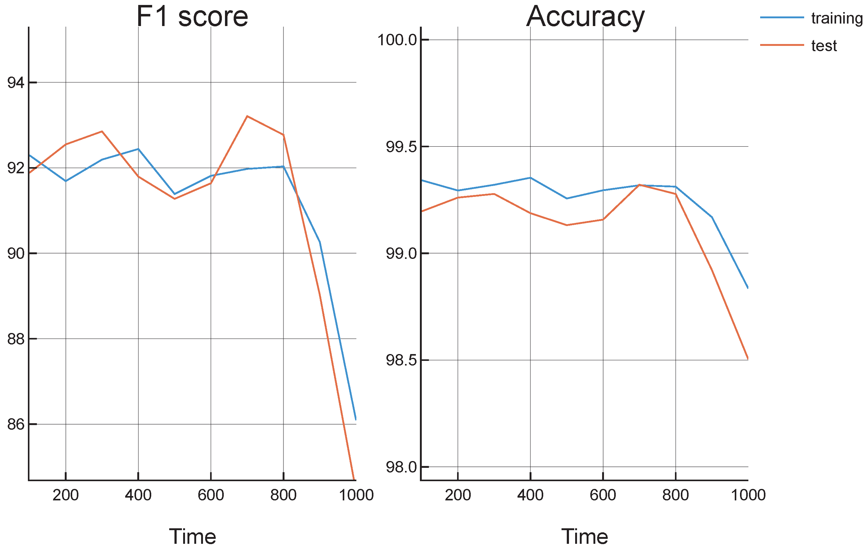
However, in this work, the application of VAEs is performed not only to codify and reconstruct a part of a composition, but also to predict the next second of the composition. Therefore, it can be seen that two different problems are studied here: reconstruction and prediction. Figure 3 shows the F1 scores and accuracies obtained for the selected configuration and threshold value, measured separately for the 8 s reconstruction and the 1-s prediction. The figures on the left show training results, while the figures on the right show test results. The figures on the top show the F1 score while the figures on the bottom show the accuracies. As can be seen, the two figures on the top show F1 scores identical to those in Figure 2. However, these figures also show the prediction F1 scores, as well as accuracies, so the results in these two tasks can be compared. Therefore, four figures show a comparison between the different metrics in the reconstruction and prediction tasks. As was expected, the F1 score and accuracy of the prediction are lower than those of the reconstruction. However, it is slightly lower, with a small difference. Therefore, the system returns good results in both tasks: reconstruction and prediction of musical compositions from this specific author.

According to the results shown in Figure 3, the prediction of music is very accurate to the real music. In this sense, it is interesting to see if this prediction is better or worse as the prediction time is further from the last known moment. Figure 4 shows the F1 score and accuracies obtained for the different moments in the one-second prediction. As a timestep of 100 ms was used, this figure only has 10 values n the x-axis. As can be seen in this figure, the F1 score and accuracy seem not to be influenced by the moment of the prediction until it reaches the one second limit. Until that moment, it seems that there is no clear tendency about having a better or worse prediction depending on the time. However, when the one-second limit is reached, the prediction drops.

In order to further evaluate the performance of the proposed model in the prediction problem, another model was implemented which only gives as prediction copies of the last frame of the input repeatedly. In this case, the accuracy in the prediction problem was 91.37%. Comparing this number to Figure 4 (right), it can be clearly seen that this system returns much better results. As the accuracy of the new repeating model was 91.37%, most of the notes and silence are repeated. In this sense, the musical information is stored on the 8.63% parts that are not repeated. An accuracy of over 99% leads to having an error rate lower than 1%. This means that very few of the non-repeating parts were missed by the neural network.

6. Conclusions

This work shows the possibility of using VAEs for music processing to solve two different problems: music codification and reconstruction, and music prediction. Two different metrics have been used, and, as the results show, both problems have been successfully solved since the results are very high in both metrics. As could be imagined, the prediction problem shows worse results than the reconstruction problem. However, these results are only slightly worse. This means that the learned features can make accurate predictions.

Therefore, it can be concluded that the features learned from the VAE can correctly be used to continue the composition similarly as the composer could have done. Moreover, this system was developed so that the decodification of the features corresponding to a specific part leads to having the following second of music. This process can be consecutively repeated with an overlap of 1 s. As a result, a whole composition can be represented in the latent space as a trajectory between different vectors in this space. Further analysis of these trajectories can give new insights about the composition and style of different authors, for example, comparing the latent spaces of the codification for two different composers can determine the similarities between them or the difference in complexity.

The development with a small dataset is one of the most prominent features of this work. Although this could be considered as a big drawback for the training of the VAE, test results are comparable to training results for both considered metrics. Therefore, the systems behave correctly with unseen pieces of music, returning their features in the latent space, and giving a prediction of the following second. However, we can not affirm that the parameters of these VAEs can be generalized to other datasets with compositions from other authors; the system should be re-trained for them.

The system described in this work was applied to compositions of only one author. Further research is still to be done in order to apply this system to different authors and/or styles. As a result, this system could be used by the community of media artists in order to help them to create new compositions or improve their compositions.

7. Future Works

From the work presented in this paper, different directions can be taken. First, in the modeling of the audio, the velocity (volume) has not been taken into account. A new model could be developed in which the output of each neuron, a real value between 0 and 1, can be interpreted as the volume of that pith in that specific moment.

As was already explained in Section 6, a musical composition can be represented as a trajectory in the latent space. This system could be trained with compositions from different authors. When high enough accuracies were obtained in both training and test sets, these trajectories could be analyzed in order to discover the differences between authors. This could be mixed with a clustering technique to discover interesting patterns in music composition. Alternatively, some researchers, such as [40], have pointed out the need for new metrics to evaluate the music generated by VAEs.

Finally, as shown in Section 5, the prediction seems to drop when it is getting to 1 s. Further studies should be carried out in order to find out if this prediction can be improved with bigger network architecture.