Design and Verification of an Interval Type-2 Fuzzy Neural Network Based on Improved Particle Swarm Optimization


Abstract
1. Introduction
2. Structure of IT2FNN
- Layer 1:
- This layer is the input layer, and each node is an input node. Only the input signal is passed to the next layer of the network.
- Layer 2:
- This layer is the membership function layer that performs the fuzzification operations. Each node is defined as a type-2 fuzzy set. Each membership function is a Gaussian membership function represented by an uncertain mean [,] and a fixed standard deviation (STD) . The function is expressed as follows:where and represent the ith input of the j-term mean and standard Gaussian membership function, respectively. The footprint of uncertainty of the Gaussian membership function represents a bounded interval of the upper membership function and lower membership function . The output of each node in the second layer represents an interval . The formula for calculating the membership degree is as follows:and
- Layer 3:
- This layer is also called the firing layer, and each node is a rule node; an algebraic product calculation is used to receive the firing strength of each rule node and .where and represent the firing strength of the rule corresponding to the upper and lower boundaries of the interval.
- Layer 4:
- This layer is called consequent layer and generates type-1 fuzzy sets through a type-reducer operation. In this layer, a numerical output is obtained after defuzzification process. The center of sets type-reducer was used to reduce the computational complexity of the type-reducer process [29]. The formula is as follows:This method simplifies the type-reducer process and only considers the combination of upper and lower boundary firing strength. The combination of firing strength and the corresponding output are expressed as follows:andwhere is obtained from the nonlinear combination of the FLNN input variables , is the link weight of each node in the FLNN, and is the function extension of the input variable. The function expansion consists of the basis functions of trigonometric polynomials.where , M represents the number of basis functions, and N represents the number of input variables.
- Layer 5:
- This layer is the output layer, and the type-reducer operation is performed on the previous layer. An interval type output is obtained. Finally, defuzzification is completed by calculating the average of and , and the NN crisp value of output y is obtained.
3. Proposed Improved Particle Swarm Optimization
- (1)
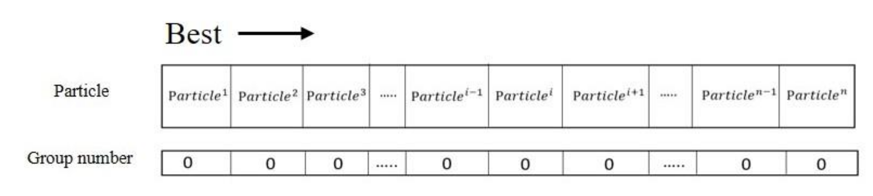
- Step 1: Coding
- (2)
- Step 2: Sorting
- (3)
- Step 3: Calculate the Similarity Threshold
- (4)
- Step 4: Particle Grouping
- (5)
- Step 5: Determine Whether to End Grouping
- (6)
- Step 6: Updating Particles Cooperatively
- (7)
- Step 7: Whether the Terminal Condition is Reached
4. Experimental Results
4.1. Dynamic System Identification
4.2. Chaotic Time-Series Prediction
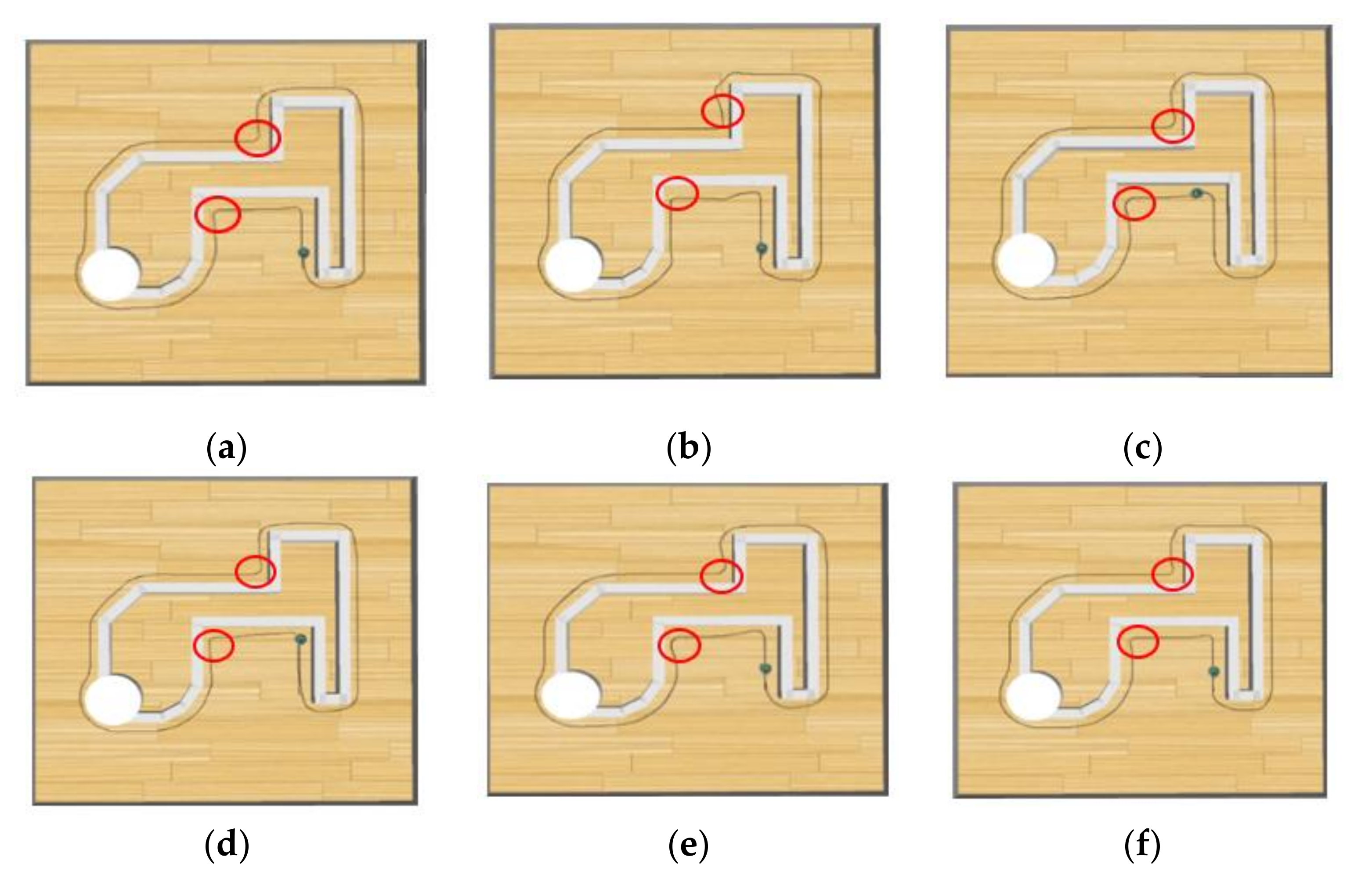
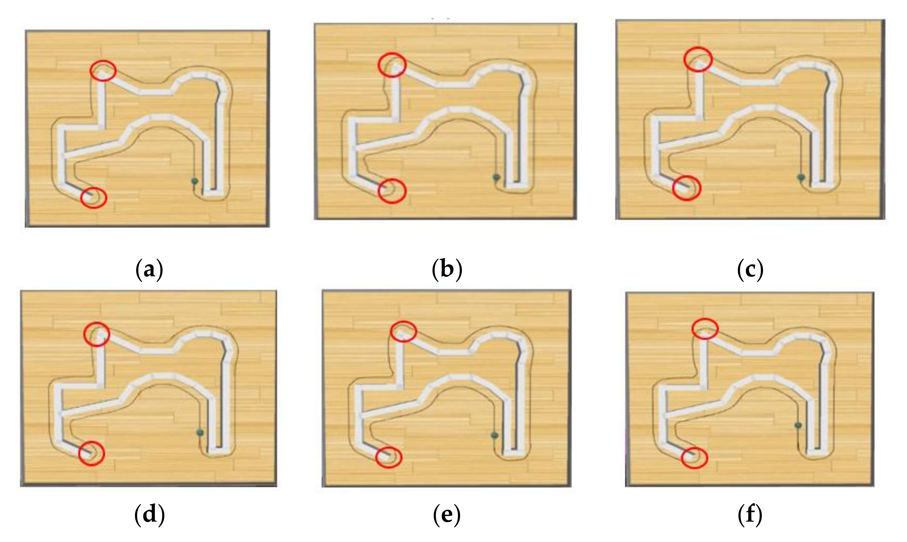
4.3. Wall-Following Control of a Mobile Robot
- The mobile robot moves more distance in the training setting than the distance of a circle around the training setting (only one circle of the training setting), indicating that the mobile robot successfully circled the training setting.
- One sensor of the mobile robot measures a distance of less than 1 cm. Figure 18a illustrates a collision between the mobile robot and the wall.
- A sensor to the side of the mobile robot detects a distance greater than 6 cm, indicating that the mobile robot has deviated from the wall, as depicted in Figure 18b.
- Total distance the mobile robot moved: The closer the moving distance of the mobile robot is to the predefined value , the closer the mobile robot is to completing one circle around the training setting.If , then the mobile robot successfully circumvents the training setting under all conditions. If , then the fitness function is zero.
- The distance the mobile robot maintained from the wall: The fitness function is the average value of WD(t) during the moving time. The aim is to maintain a fixed distance between the mobile robot and the wall. In each time step, the distance WD(t) between the side of the mobile robot and the wall is calculated as follows:where is the expected distance of the robot from the wall. A predefined distance was set to 4 cm, as shown in Figure 19a, and is the time step of the mobile robot during the learning process of the wall-following motion. If the mobile robot maintains a fixed expected distance from the wall, then the value of is equal to zero.
- The degree of parallelism between the mobile robot and the wall: The fitness function was used to evaluate the degree of parallelism between the mobile robot and the wall. If the robot was parallel to the wall, then the angle between the sensor on the right side of the mobile robot and the wall was 90°. According to the law of cosines, must be equal to , forming an isosceles triangle, as depicted in Figure 19b. The formulas are expressed as follows:where and are the distances of the mobile robot sensors, and r is the radius of the mobile robot. The fitness function is defined as the average value of the degree of parallelism between the mobile robot and the wall during the moving time. If the mobile robot is parallel to the wall, then the value of is equal to zero.Therefore, a fitness function F (·) was used to evaluate overall control performance. This fitness function was formed by combining the aforementioned subfitness functions () as follows:This proposed DGCPSO was compared with other evolutionary algorithms. Table 5 lists the initial parameter settings of DGCPSO. To evaluate the algorithm stability, the experiment was performed ten times for each algorithm.
5. Conclusions
- (1)
- The proposed DGCPSO uses the dynamic grouping and cooperative particle swarm optimization to improve search capabilities and reach near global optimum;
- (2)
- Interval type-2 fuzzy sets are used in IT2FNN to reduce sensor-sensing noise and disturbance;
- (3)
- The effectiveness and robustness of the proposed method are improved in identification, prediction, and control problems.
Author Contributions
Funding
Conflicts of Interest
References
- Qi, C.; Fourie, A.; Chen, Q. Neural network and particle swarm optimization for predicting the unconfined compressive strength of cemented paste backfill. Constr. Build. Mater. 2018, 159, 473–478. [Google Scholar] [CrossRef]
- Naung, Y.; Schagin, A.; Oo, H.L.; Ye, K.Z.; Khaing, Z.M. Implementation of data driven control system of DC motor by using system identification process. In Proceedings of the 2018 IEEE Conference of Russian Young Researchers in Electrical and Electronic Engineering (EIConRus), Moscow, Russia, 29 January–1 February 2018. [Google Scholar] [CrossRef]
- Cupertino, F.; Giordano, V.; Naso, D.; Delfine, L. Fuzzy control of a mobile robot. IEEE Robot. Autom. Mag. 2006, 13, 74–81. [Google Scholar] [CrossRef]
- Zhu, M.; Wang, X.; Wang, Y. Human-like automous car-following model with deep reinforcement learning. Transp. Res. Part C Emerg. Technol. 2018, 97, 348–368. [Google Scholar] [CrossRef]
- Anish, P.; Parhi, D.R. Multiple mobile robots navigation and obstacle avoidance using minimum rule based ANFIS network controller in the cluttered environment. Int. J. Adv. Robot. Autom. 2016, 1, 1–11. [Google Scholar]
- Masmoudi, M.S.; Krichen, N.; Masmoudi, M.; Derbel, N. Fuzzy logic controllers design for omnidirectional mobile robot navigation. Appl. Soft Comput. 2016, 49, 901–919. [Google Scholar] [CrossRef]
- Hidalgo, D.; Castillo, O.; Melin, P. Type-1 and type-2 fuzzy inference systems as integration methods in modular neural networks for multimodal biometry and its optimization with genetic algorithms. Inf. Sci. 2009, 179, 2123–2145. [Google Scholar] [CrossRef]
- Kayacan, E.; Khanesar, M.A. Chapter 2: Fundamentals of Type-1 Fuzzy Logic Theory. Fuzzy Neural Netw. Real Time Control Appl. 2016, 2, 13–24. [Google Scholar]
- Kayacan, E.; Khanesar, M.A. Chapter 3: Fundamentals of Type-2 Fuzzy Logic Theory. Fuzzy Neural Netw. Real Time Control Appl. 2016, 3, 25–35. [Google Scholar]
- Maguire, L.P.; Roche, B.; McGinnity, T.M.; McDaid, L.J. Predicting a chaotic time series using a fuzzy neural network. Inf. Sci. 1998, 112, 125–136. [Google Scholar] [CrossRef]
- Sarabakha, A.; Fu, C.; Kayacan, E. Intuit before tuning: Type-1and type-2 fuzzy logic controllers. Appl. Soft Comput. 2019, 81, 105495. [Google Scholar] [CrossRef]
- Castillo, O.; Melin, P.; Kacprzyk, J.; Pedrycz, W. Type-2 Fuzzy Logic: Theory and Applications. In Proceedings of the 2007 IEEE International Conference on Granular Computing (GRC 2007), Fremont, CA, USA, 2–4 November 2007. [Google Scholar] [CrossRef]
- Castillo, O.; Melin, P. Comparison of hybrid intelligent systems, neural networks, and interval type-2 fuzzy logic for time series prediction. In Proceedings of the International Joint Conference on Neural Networks, Orlando, FL, USA, 12–17 August 2007; pp. 3086–3091. [Google Scholar]
- El-Nagar, A.M.; El-Bardini, M. Interval type-2 fuzzy neural network controller for a multivariable anesthesia system based on a hardware-in-the-loop simulation. Artif. Intell. Med. 2014, 61, 1–10. [Google Scholar] [CrossRef] [PubMed]
- Kim, C.J.; Chwa, D. Obstacle Avoidance Method for Wheeled Mobile Robots Using Interval Type-2 Fuzzy Neural Network. IEEE Trans. Fuzzy Syst. 2015, 23, 677–687. [Google Scholar] [CrossRef]
- Mendel, J.M. General Type-2 Fuzzy Logic Systems Made Simple: A Tutorial. IEEE Trans. Fuzzy Syst. 2013, 22, 1162–1182. [Google Scholar] [CrossRef]
- Liu, F. An efficient centroid type-reduction strategy for general type-2 fuzzy logic system. Inf. Sci. 2008, 179, 2224–2236. [Google Scholar] [CrossRef]
- Sharifian, A.; Ghadi, M.J.; Ghavidel, S.; Li, L.; Zhang, J. A new method based on Type-2 fuzzy neural network for accurate wind power forecasting under uncertain data. Renew. Energy 2018, 120, 220–230. [Google Scholar] [CrossRef]
- Adigun, O.; Kosko, B. Training Generative Adversarial Networks with Bidirectional Backpropagation. In Proceedings of the 2018 17th IEEE International Conference on Machine Learning and Applications (ICMLA), Orlando, FL, USA, 17–20 December 2018; pp. 1178–1185. [Google Scholar]
- Hou, Y.; Zhao, L.; Lu, H. Fuzzy neural network optimization and network traffic forecasting based on improved differential evolution. Future Gener. Comput. Syst. 2018, 81, 425–432. [Google Scholar] [CrossRef]
- Gu, P.; Xiu, C.; Cheng, Y.; Luo, J.; Li, Y. Adaptive ant colony optimization algorithm. In In Proceedings of the IEEE 2014 International Conference on Mechatronics and Control (ICMC), Jinzhou, China, 3–5 July 2014; Volume 6, pp. 6–8. [Google Scholar]
- Chen, X.; Wei, X.; Yang, G.; Du, W. Fireworks explosion based artificial bee colony for numerical optimization. Knowl.-Based Syst. 2020, 188, 105002. [Google Scholar] [CrossRef]
- Mirjalili, S.; Lewis, A. The Whale Optimization Algorithm. Adv. Eng. Softw. 2016, 95, 51–67. [Google Scholar] [CrossRef]
- Gong, W.; Cai, Z. Differential Evolution with Ranking-Based Mutation Operators. IEEE Trans. Cybern. 2013, 43, 2066–2081. [Google Scholar] [CrossRef]
- Cai, X.; Gao, L.; Li, F. Sequential approximation optimization assisted particle swarm optimization for expensive problems. Appl. Soft Comput. 2019, 83, 105659. [Google Scholar] [CrossRef]
- Gan, W.; Zhu, D.; Ji, D. QPSO-model predictive control-based approach to dynamic trajectory tracking control for unmanned underwater vehicles. Ocean Eng. 2018, 158, 208–220. [Google Scholar] [CrossRef]
- Liu, X.F.; Zhou, Y.R.; Yu, X. Cooperative particle swarm optimization with reference-point-based prediction strategy for dynamic multiobjective optimization. Appl. Soft Comput. 2020, 87, 105988. [Google Scholar] [CrossRef]
- Chang, J.Y.; Lin, Y.Y.; Han, M.F.; Lin, C.T. A functional-link based interval type-2 compensatory fuzzy neural network for nonlinear system modeling. In Proceedings of the 2011 IEEE International Conference on Fuzzy Systems (FUZZ-IEEE 2011), San Diego, CA, USA, 8–12 March 2011; pp. 939–943. [Google Scholar]
- Mendel, J.M. Type-2 fuzzy sets and systems: An overview. IEEE Comput. Intell. Mag. 2007, 2, 20–29. [Google Scholar] [CrossRef]


| NP | ω | Generation | Rule | ||
|---|---|---|---|---|---|
| 30 | 0.3 | 2 | 2 | 200 | 6 |
| Algorithm | DGCPSO | Differential Evolution (DE) [24] | Particle Swarm Optimization (PSO) [25] | Quantum-Based PSO (QPSO) [26] | Cooperative PSO (CPSO) [27] | |
|---|---|---|---|---|---|---|
| Fitness | ||||||
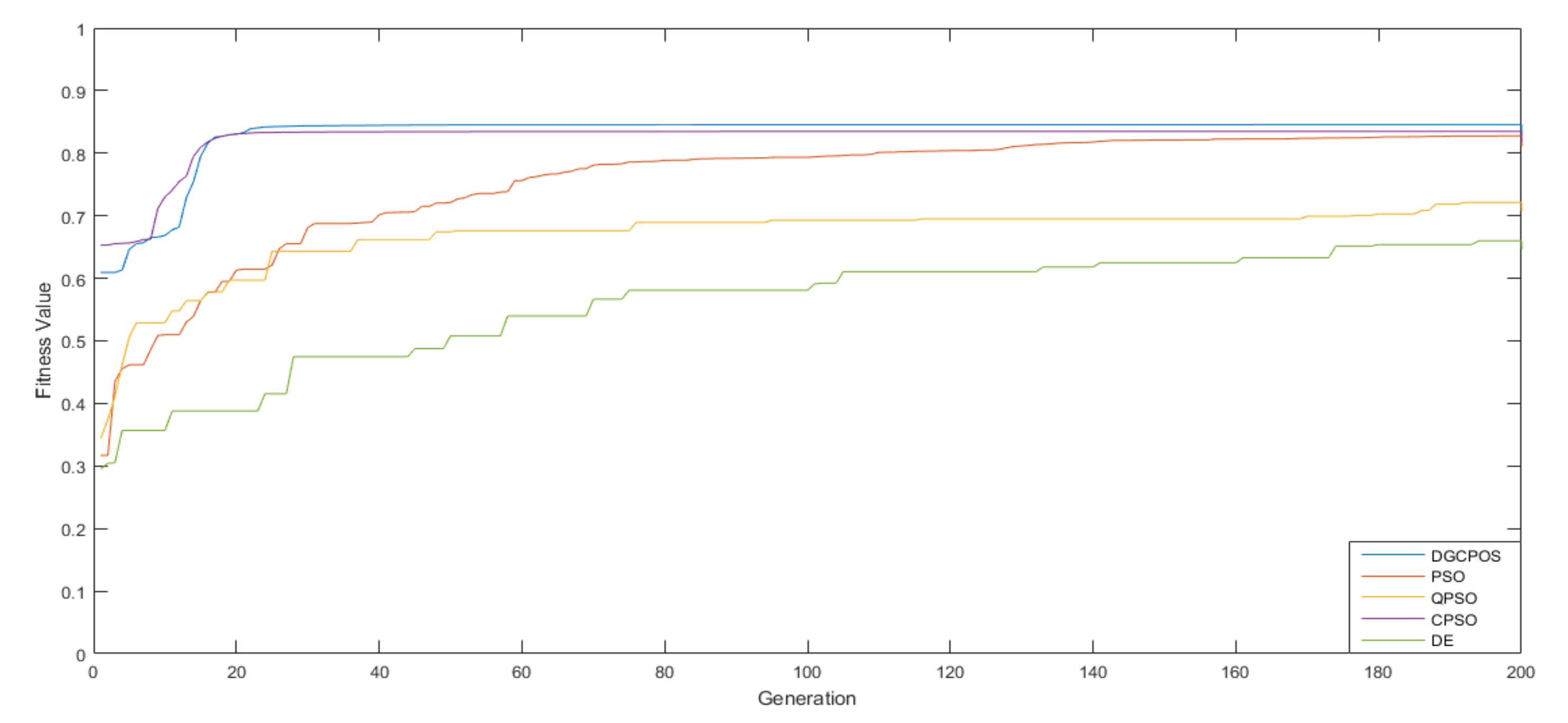
| Best | 0.851 | 0.830 | 0.844 | 0.810 | 0.834 | |
| Worst | 0.833 | 0.793 | 0.823 | 0.750 | 0.612 | |
| Average | 0.842 | 0.811 | 0.831 | 0.770 | 0.690 | |
| Standard deviation (SD) | 0.002 | 0.009 | 0.003 | 0.015 | 0.105 | |
| NP | ω | Generation | Rule | ||
|---|---|---|---|---|---|
| 30 | 0.3 | 2 | 2 | 200 | 6 |
| Algorithm | DGCPSO | DE [24] | PSO [25] | QPSO [26] | CPSO [27] | |
|---|---|---|---|---|---|---|
| Fitness | ||||||
| Best | 0.990 | 0.987 | 0.981 | 0.984 | 0.983 | |
| Worst | 0.987 | 0.979 | 0.962 | 0.960 | 0.952 | |
| Average | 0.984 | 0.980 | 0.973 | 0.974 | 0.972 | |
| SD | 0.004 | 0.006 | 0.005 | 0.006 | 0.005 | |
| NP | ω | Generation | Rule | ||
|---|---|---|---|---|---|
| 30 | 0.3 | 2 | 2 | 3000 | 6 |
| Algorithm | Fitness Value | Number of Successful Runs (NSR) | |||
|---|---|---|---|---|---|
| Best | Worst | Average | SD | ||
| DGCPSO | 0.942 | 0.905 | 0.922 | 0.004 | 10 |
| Artificial Bee Colony (ABC) [22] | 0.862 | 0.794 | 0.837 | 0.004 | 8 |
| Whale Optimization Algorithm (WOA) [23] | 0.933 | 0.826 | 0.872 | 0.015 | 8 |
| DE [24] | 0.848 | 0.824 | 0.853 | 0.005 | 10 |
| PSO [25] | 0.932 | 0.844 | 0.901 | 0.005 | 10 |
| QPSO [26] | 0.937 | 0.867 | 0.921 | 0.002 | 10 |
© 2020 by the authors. Licensee MDPI, Basel, Switzerland. This article is an open access article distributed under the terms and conditions of the Creative Commons Attribution (CC BY) license (http://creativecommons.org/licenses/by/4.0/).
Share and Cite
Lin, C.-J.; Jeng, S.-Y.; Lin, H.-Y.; Yu, C.-Y. Design and Verification of an Interval Type-2 Fuzzy Neural Network Based on Improved Particle Swarm Optimization. Appl. Sci. 2020, 10, 3041. https://doi.org/10.3390/app10093041
Lin C-J, Jeng S-Y, Lin H-Y, Yu C-Y. Design and Verification of an Interval Type-2 Fuzzy Neural Network Based on Improved Particle Swarm Optimization. Applied Sciences. 2020; 10(9):3041. https://doi.org/10.3390/app10093041
Chicago/Turabian StyleLin, Cheng-Jian, Shiou-Yun Jeng, Hsueh-Yi Lin, and Cheng-Yi Yu. 2020. "Design and Verification of an Interval Type-2 Fuzzy Neural Network Based on Improved Particle Swarm Optimization" Applied Sciences 10, no. 9: 3041. https://doi.org/10.3390/app10093041
APA StyleLin, C.-J., Jeng, S.-Y., Lin, H.-Y., & Yu, C.-Y. (2020). Design and Verification of an Interval Type-2 Fuzzy Neural Network Based on Improved Particle Swarm Optimization. Applied Sciences, 10(9), 3041. https://doi.org/10.3390/app10093041