State Estimation for DC Microgrids using Modified Long Short-Term Memory Networks

Abstract

The development of state estimators for local electrical energy supply systems is inevitable as the role of the system’s become more important, especially with the recent increased interest in direct current (DC) microgrids. Proper control and monitoring requires a state estimator that can adapt to the new technologies for DC microgrids. This paper mainly deals with the DC microgrid state estimation (SE) using a modified long short-term memory (LSTM) network, which until recently has been applied only in forecasting studies. The modified LSTM network for the proposed state estimator adopted a specifically weighted least square (WLS)-based loss function for training. To demonstrate the performance of the proposed state estimator, a comparison study was done with other SE methods included in this paper. The results showed that the proposed state estimator had high accuracy in estimating the states of DC microgrids. Other than the enhanced accuracy, the deep-learning-based state estimator also provided faster computation speeds than the conventional state estimator.

1. Introduction

State estimation (SE) is an important component of an energy management system (EMS), since it allows the system operator to control and monitor an electric power system [1]. The state of a power system can be estimated based on the supervisory control and data acquisition (SCADA) measurements, phasor measurement unit (PMU) measurements, and a topology processor. Some of the most important functions of EMS are based on the SE, such as contingency analysis, optimal power flow, and security assessment [2,3]. Measurement data obtained straight from the telemetry is usually not perfect, as random errors are always present. These kinds of measurements need to be processed by SE to get the closest approximation to the real value before being used by the EMS functions. This fortifies the importance of SE in the transmission system level of power systems [4].

In the last decade, there has been a paradigm shift in the distribution system technology. The conventional unidirectional model had changed as the consumers in the distribution system have evolved from passive users to active users [5]. Around the same period, the concept of microgrids started to emerge as an alternative solution for local energy systems with distributed energy resources [6]. The introduction of microgrids led to distribution systems that are more active, with more diverse dynamics and service-oriented actions compared to their predecessor. This phenomenon established a need to bring distribution systems into the operation control and monitoring circle. Consequently, the development of microgrid SE is inevitable. However, due to the differences of the transmission and distribution systems [7,8], the tools used for transmission system SE (TSSE) might not be directly applicable for microgrids and would need some adjustment for microgrid SE application.

One of the main problems in microgrid SE applications is the lack of available real-time measurements in microgrids. As a result, the input data required by the observability analysis in the SE process is not sufficient. One of the ideas to solve the measurement scarcity problem is the use of pseudo-measurements [1,9]. Pseudo-measurements are usually generated using the daily load profile (DLP) with annual updates [10]. Nowadays, the presence of advanced metering infrastructure (AMI) might help in providing a more accurate definition of DLP, which could lead to improved pseudo-measurements [11], and as a result, a more accurate microgrid SE.

Conventionally, state estimators are formulated as overdetermined systems of nonlinear equations, which are then solved by using the weighted least squares (WLS) method [1,12]. Conventional SE use the measurement data acquired at the present time to estimate the state of the system. In [13], a fuzzy linear SE model based on Tanaka’s fuzzy linear regression model was employed to model the uncertainty in the system. In [14], a decentralized SE method was proposed for hybrid microgrids using a dual decomposition approach, where the estimation was separately conducted for either grid, with only limited information exchanged during the process. In [15], a state estimator was developed with centralized and decentralized approaches for hybrid alternating current (AC)/high voltage DC (HVDC) grids. The optimization-oriented state estimators were proven to be functional and stable, but in terms of computational speed and accuracy further improvement is desired. In [16], a fast real-time state estimator based on the belief propagation algorithm was proposed. The model proved to be robust against ill-conditioned scenarios caused by the differences between various measurements.

Different efforts towards a fast real-time SE were introduced in [17], where the artificial neural network (ANN) method was used for a smart grid SE. Another effort using a deep learning-based state estimator is shown in [18], which combines the use of a deep neural network (DNN) for TSSE and a recurrent neural network (RNN) for state forecasting. With the offline training phase, the state estimator proved to be able to run in real time with affordable training and minimal tuning, which resulted in improved performance compared with existing alternatives. In [19], a shallow neural network is used in a distribution system state estimator to produce an approximation of the system’s state. The state is then sent into the Gauss–Newton algorithm for refinements, which results in fast convergence to an optimal solution of SE. Different deep learning methods for distribution grid SE were tested in [20]. In the literature, an auto-associative neural network (AANN), or autoencoder-based state estimator, was shown to have the advantage of being independent of the network parameters and topology, which resulted in effective and accurate estimation.

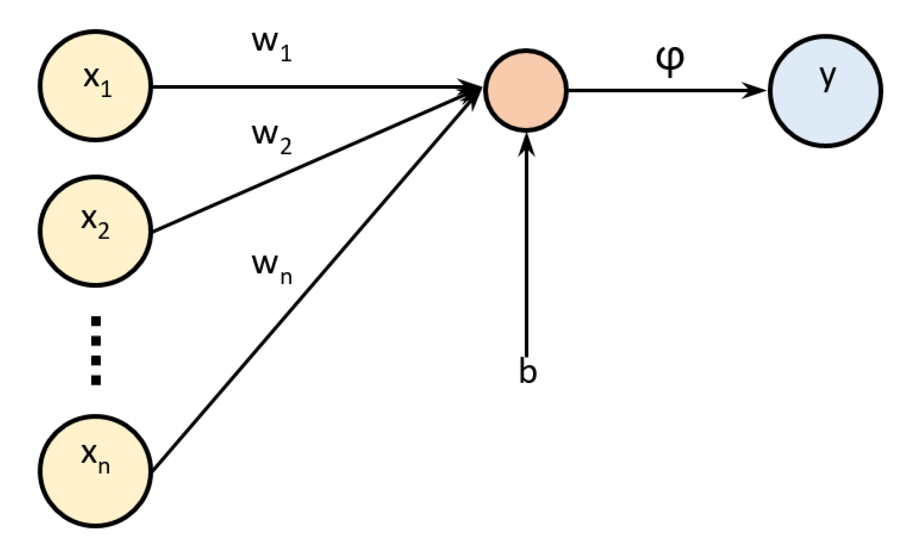
In electric power systems, deep learning applications are not limited to SE only. A multilayer perceptron (MLP) neural network was adopted in [21] for short-term load forecasting, which produces minimal estimation errors. Another deep learning method, namely the long short-term memory (LSTM) network, was used in [22] for residential load forecasting, which outperformed the listed rival algorithm in forecasting individual residential households in terms of forecasting performance. Meanwhile, in [23], LSTM was used to forecast solar irradiance for microgrids based on widely available weather data only. The literature showed higher accuracy compared to the simple feedforward neural network (FFNN) method.

From all the previous works, one can notice that neural networks and deep learning approaches can provide better results over the conventional methods in some applications in terms of accuracy and computational speed. Additionally, in microgrid SE, one problem with the conventional method is the usage of pseudo-measurement. Out of several measurement types used as the SE input, the pseudo-measurement has the highest error variance, which could cause a sub-optimal SE result. For application of the deep learning method for SE in the microgrid system, the historical data is used in the training process of the state estimator, unlike the conventional WLS SE, which only uses the present time data. However, even though both methods used pseudo-measurement, the deep learning method training process disregarded the error variance of all measurement types. Hence, the deep learning method, if applied for SE in microgrid systems, might give improved SE results.

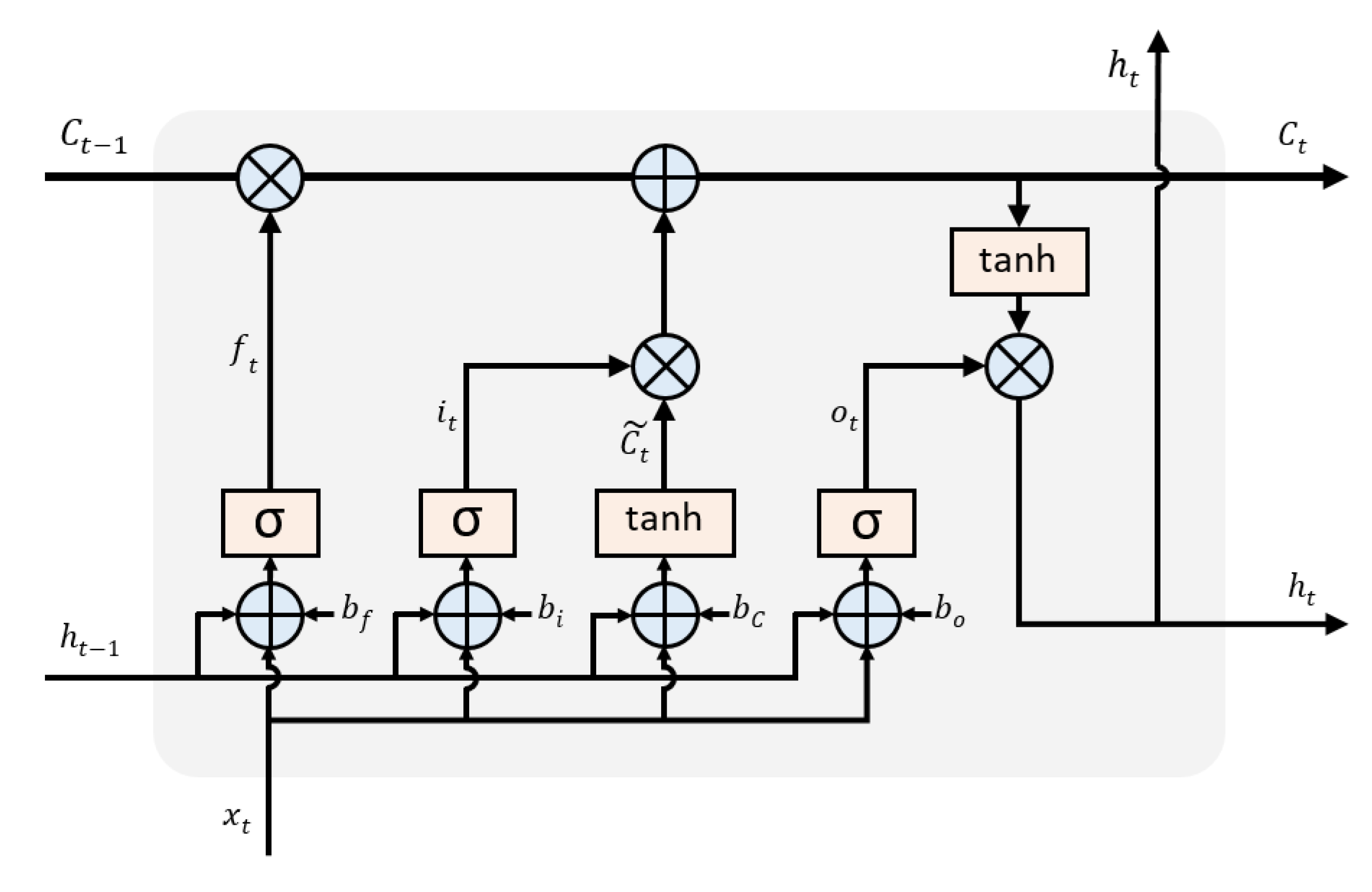
A lot of studies have been done on SE, such as TSSE, distribution system SE, and microgrid SE in general. However, not many studies have discussed DC microgrid SE. In particular, this paper proposes a DC microgrid state estimator using a modified LSTM network. LSTM is chosen as its structure allows the capability to learn the long-term dependencies in sequential data [24,25,26]. This ability makes LSTM especially good at learning time-series data, which conveniently, in the case of microgrid SE, is the structure of the measurement data as the historical data. LSTM predicts an output based on the current input and previous calculated output. In comparison, MLP only considers the current input to predict an output and does not utilize its previous output to improve its prediction accuracy. Furthermore, there had not been any previous attempt at using the LSTM method for SE.

To estimate the state of a DC microgrid, measurements of the bus voltage magnitude and current flow are collected to train our LSTM state estimator. Additionally, in order to demonstrate the algorithm’s ability to solve the observability problem in microgrid systems, the pseudo-measurements are included to increase the accuracy of the SE. In this paper, a loss function resembling the objection function of the conventional WLS state estimator is used to train the network model. A set of weights is applied to the loss function, in which certain weight values correspond to certain measurement types. The same simulation schemes are applied to the other methods of SE (e.g., conventional WLS, MLP-based, and normal LSTM-based SE) as a comparison to validate the performance of the proposed modified LSTM-based SE.

The contributions of this paper in comparison with the existing literature can be summarized as follows:

• The paper investigated a deep-learning-based state estimator for DC microgrids.
• The state estimator adopted the LSTM network method, which until recently has only been applied in forecasting studies.
• The LSTM for the state estimation of DC microgrids was modified to obtain better performance, using WLS-based loss function for training.

The rest of this paper is structured as follows. In Section 2, the background of the conventional SE method for electrical power systems is explained. Section 3 covers the basics of deep learning methods, such as multilayer perceptron (MLP) and LSTM networks. Further discussion about SE for DC systems, the system configuration used for simulation, and the types of measurements for SE are presented in Section 4. Section 5 gives an overview of the proposed state estimator. The simulation outcomes of the previously studied and the proposed state estimators are then demonstrated and discussed in Section 6 and Section 7, respectively. Finally, the conclusion is presented in Section 8.

2. Conventional WLS SE Method

SE is an algorithm used to determine a close approximation of the system’s actual state from raw measurement data that is corrupted by noise. The WLS method is one of the most common methods adopted for SE [1,12]. The weight in the WLS method is introduced into the algorithm to emphasize trusted measurements and de-emphasize less-trusted measurements. The WLS method is based on a nonlinear optimization problem that minimizes the squared error of the measurement while taking into account the error variance of different measurement types. The general measurement model for SE is written as

$$z=h\left(x\right)+e,$$

(1)

where $z$ is the measurement vector, $x$ is the true state vector, $h\left(x\right)$ is the function linking the measurement to the state, and $e$ is the measurement error, which is assumed to have zero mean and variance ${\sigma }_N^2$. The complex nodal voltage is a commonly used variable in SE [1]. The true state vector $x$ is written as

$$x=\left[\begin{array}{c}{V}_N\\ {\mathsf{\theta }}_N\end{array}\right],$$

(2)

where $V_N$ is the voltage magnitude and ${\theta }_N$ is the voltage angle.

The WLS method calculates the system’s state by iteratively minimizing the cost function

$$J={\displaystyle \sum }_{i=1}^N\frac{{\left(z_i-h_i\left(x\right)\right)}^2}{{\sigma }_i^2}={\left[z-h\left(x\right)\right]}^T·W·\left[z-h\left(x\right)\right],$$

(3)

where ${\sigma }_i^2$ is the error variance and $N$ is the number of measurements [1,12,15]. The weighting matrix $W$ is equal to the inverse of the error variance matrix $R\in {ℝ}^{N\times N}$. The Gauss–Newton algorithm is used to minimize the cost function (Equation (3)). The algorithm is calculated iteratively, resulting in the normal equation being written as

$$G\Delta x=H^T·W·\left(z-h\left(x\right)\right),$$

(4)

where$H$ is the Jacobian matrix of the measurement function $h\left(x\right)$. The gain matrix $G$ in Equation (4) is defined as $G=H^T·W·H$. The state estimate $x^{k+1}$ is calculated using the vector $\Delta x$ for each iteration $k$ by the following equation, which is written as

$$x^{k+1}=x^k+\Delta x.$$

(5)

The iteration process will stop and give the state estimate result when $\Delta x^T\Delta x<ϵ$ is reached, where $ϵ$ is the desired accuracy.

3. Deep Learning Theoretical Background

Deep learning is a subset of machine learning that uses multiple layers of the algorithm to learn the data representation to extract higher level features from a raw input. Deep learning evolved from artificial neural networks, which have existed since the 1940s [24]. As MLP and LSTM methods are used in our simulation, both deep learning methods will be explained in detail in this section.

3.1. MLP Network

MLP is a class of FFNN. The term MLP or “multilayer perceptron”, refers to a number of perceptrons that are organized into several layers [24]. A single perceptron can calculate one output from multiple inputs by mathematically making a linear combination [25,27]. A perceptron is illustrated in Figure 1. In the figure, $x$ is denoted as the input signal vector, $w$ as the weight vector, $b$ as the bias, and $y$ as the output. The output $y$ can be obtained by putting the weighted sum of $x$, $w$, and $b$ into the activation function $\phi$ [23,25]. The equation is written as

$$y=\phi \left({\displaystyle \sum }_{i=1}^n{w}_i{x}_i+b\right).$$

(6)

Several perceptron can be used as the building blocks for a more structurally complex MLP since one perceptron has a limited ability to map the output. Conventionally, an MLP is composed of at least three layers, which are the input layer, the hidden layer, and the output layer. Each layer can have several neurons or nodes. Consider an MLP with one hidden layer illustrated in Figure 2. The calculation for each layer is done in a similar manner to Equation (6), and it can be written as

$$z=\phi \left({\displaystyle \sum }_{j=1}^n{w}_{{~}_j}\left({\displaystyle \sum }_{i=1}^m{w}_{j_i}{x}_i+b_j\right)+b_{~}\right),$$

(7)

where $z$ is the output vector; $x$ is the input vector; $w_{j_i}$ and $b_j$ are the weight matrix and the bias vector of the input layer, respectively; $w_{{~}_j}$ and $b_{~}$ are the weight matrix and the bias vector of the hidden second layer, respectively; and $\phi$ is the activation function. The nonlinear activation function can be either sigmoid, tanh, rectified linear unit (ReLU), etc [28].

The MLP network can be trained using a supervised learning technique called the backpropagation algorithm [25,27,29]. The backpropagation algorithm is composed of two steps—the forward pass and the backward pass. The forward pass would calculate the predicted output with the corresponding input using Equation (7). At the end of the forward step, an error would be obtained by calculating the predicted output and the real output difference. The error would be evaluated with a cost function. Next, in the backward pass, the partial derivative of the cost function with respect to different parameters would be calculated and propagated back through the network with chain rule. Based on the result, the model would adjust the parameters for the highest accuracy. The weight of the network would be adjusted using gradient-based optimization. This whole process would be done iteratively until the weight values converge or the weight value that would minimize the error is found [25].

3.2. Long Short-Term Memory Network

The LSTM network is a special type of RNN that is capable of learning long-term dependencies. The LSTM network structure allows it to learn the correlation between an output based on the current input and the previous calculated output. Hence, LSTM is good at processing and predicting sequential data such as time-series data. LSTM was developed by Hochreiter and Schmidhuber in 1997 [30]. LSTM is modeled similarly to a chain of repeating modules of neural networks. LSTM does not suffer much from vanishing or exploding gradient problems, as with RNNs, because of the inclusion of the forget gate $f_t$ and the dependency of the current cell state to the forget gate [24,26]. Typically, LSTM is composed of a cell state, a forget gate, an input gate, and an output gate.

Figure 3 illustrates a single LSTM unit, as discussed in [23,24]. The important part of LSTM is the cell state $C_t$, which acts as a memory that stores values for a period of time. The cell state $C_t$ is regulated by three gates composed of a sigmoid function, which gives output values of between 0 and 1 [23,24,26]. At time step $t$, the forget gate layer $f_t$ would assess the input $x_t$ and the previous step’s hidden state $h_{t-1}$ in order to decide which information would be forgotten from the cell state $C_{t-1}$. A value between 0 and 1 would be assigned for each element in the cell state vector $C_{t-1}$. The value 0 would indicate that the LSTM should forget the state, while the value 1 would mean that the state should be kept. The forget gate equation is written as

$$f_t=\sigma \left(W_f{h}_{t-1}+U_f{x}_t+b_f\right).$$

(8)

Afterward, the input gate would decide which cell unit would be updated by giving an output of between 0 and 1, using the equation

$$i_t=\sigma \left(W_i{h}_{t-1}+U_i{x}_t+b_i\right).$$

(9)

Then, the candidate set of new values would be calculated for the cell state using $x_t$ and $h_{t-1}$, with the equation written as

$$\widetilde{C_t}=tanh \left(W_C{h}_{t-1}+U_C{x}_t+b_C\right).$$

(10)

The new cell state $C_t$ would then be updated with the equation

$$C_t=f_t\ast C_{t-1}+i_t\ast \widetilde{C_t}.$$

(11)

In order to determine which cell state to output, $x_t$ and $h_{t-1}$ would be passed through the output gate, which would give an output value of between 0 and 1 for each component in the cell state $C_t$, with the equation written as

$$o_t=\sigma \left(W_o{h}_{t-1}+U_o{x}_t+b_o\right).$$

(12)

The updated hidden state $h_t$ is then calculated by putting the cell state through a tanh function and multiplying it with output $o_t$, which is written as

$$h_t=o_t\ast tanh\left(C_t\right).$$

(13)

Note that in Equations (8)–(13), the term $f$ refers to the forget gate, $i$ refers to the input gate, $o$ refers to the output gate, and $C$ refers to the cell; all of which are of the same dimensions as the hidden vector $h$. $W$, $U$, and $b$ are the recurrent weight matrix, the input weight matrix, and the bias terms, respectively.

The LSTM network can be trained using a supervised learning technique similar to the MLP network’s backpropagation algorithm, called the backpropagation through time (BPTT) algorithm [24]. This algorithm is used for recurrent networks such as LSTM networks. The BPTT algorithm is started by unfolding a recurrent neural network in time. The unfolded network contains one input time step, one output, and one copy of the network for each time step. Next, for each time step, the loss and the corresponding error will be calculated and backpropagated. After the process is finished, the recurrent network will be folded back, and the weights will be updated. As the number of timesteps in the BPTT algorithm increases, the calculation process also become more complex, making it computationally expensive compared to the standard backpropagation algorithm.

4. DC Microgrid SE and System Configuration

4.1. SE for DC System

Since the proposed state estimator is intended for DC microgrid application, the state variable that would be used is the voltage magnitude $V_N$. The resulting vector $x_{DC}$ contains the states of all buses, which are the voltage magnitude of each bus inside the DC system, denoted as

$$x_{DC}=\left[\begin{array}{c}{V}_1\\ ⋮\\ V_N\end{array}\right],$$

(14)

with $N$ as the number of buses.

The measurements that could be considered for a DC microgrid SE are the voltage magnitude measurement, the current flow measurement, the power flow measurement, the current injection measurement, and the power injection measurement [15]. For the current and power flow measurements, the equations are written as

$$I_{flow,ij}=\left(V_i-V_j\right)·g_{ij}$$

(15)

and

$$P_{flow,ij}=V_i·\left(V_i-V_j\right)·g_{ij},$$

(16)

where $i$ is the sending bus, $j$ is the receiving bus, and $g_{ij}$ is the conductance of the line between the buses. For the current and power injection measurements on bus $i$, the equations are written as

$$I_{inj,i}={\displaystyle \sum }_{j=1}^N\left(V_i-V_j\right)·g_{ij}$$

(17)

and

$$P_{inj,i}={\displaystyle \sum }_{j=1}^N{V}_i·\left(V_i-V_j\right)·g_{ij}.$$

(18)

4.2. DC Microgrid System Configuration

In this paper, a 9-bus DC microgrid test system is designed and used for the simulation. As illustrated in Figure 4, the DC microgrid is connected to an AC utility grid by a bi-directional interlink converter (IC) at bus 8. The test system is mainly composed of loads, a battery energy storage system (BESS), and a photovoltaic (PV) system. The BESS is modeled using the electrical equivalent circuit model of a lithium-ion battery and the PV is modeled after the monocrystalline solar cell. In the simulation, the DC loads are rated at 20 kW, and are located on bus 1, bus 2, and bus 3. The BESSs are located on bus 5, bus 6, and bus 8, all with a rating of 20 kW. The PV systems are also located on bus 5, bus 6, and bus 8, with a rating of 20 kW.

In normal operation, the power consumed by the load and the power generated from generation sources inside the microgrid are balanced. Meanwhile, for fluctuating DC loads, the BESS control should solve this problem by instructing BESS to charge or discharge power. Additionally, with the addition of BESSs and PV systems, if the grid operation mode changes from grid-connected mode to islanded mode, the microgrid will be able to maintain the system stability, as it can maintain the balance between load and generation within the grid.

5. Experimental Setup of the Proposed Modified LSTM-Based State Estimator

5.1. Measurement Data Preparation for DC Microgrid SE

The Power System Computer-Aided Design (PSCAD) software is used to simulate the DC microgrid. PSCAD is a time domain simulation software for analyzing power system transience. From the PSCAD simulation, we obtained 21-day long measurement data composed of the estimation input and the target output. The time resolution for the measurement data is 5 min.

For the conventional WLS state estimator, the last day of the 21-day long measurement data is used to estimate the state of the DC microgrid. For the deep-learning-based state estimator, the 21-day long measurement data are divided into 20-day long training data and 1-day long testing data, similar to the conventional WLS state estimator.

The estimation input is used for both the conventional WLS state estimator and the deep-learning-based state estimator to estimate the system state. For the DC microgrid SE, the estimation input is composed of three measurement types: the bus voltage, the current flow, and the power injection. White Gaussian noise is also added into these measurements.

The power sources in the DC microgrid are located on bus 5, bus 6, and bus 8. Assuming that the buses with the power sources are the controlled buses, the real measurements for voltage were performed on bus 5 (V_bus5), bus 6 (V_bus6), and bus 8 (V_bus8). Measurement error of 1% was considered for the voltage measurement.

The measurements of the current flow were done on all of the lines connected to the buses with the power sources. The real measurements were done on line 5–4 (I_flow54), line 6–4 (I_flow64), line 5–7 (I_flow57), line 6–9 (I_flow69), line 8–7 (I_flow87), and line 8–9 (I_flow89). Measurement error of 3% was considered for the current flow measurement.

Assuming that there were no real measurements on the load buses, pseudo-measurements were used to get the power injection measurements. The pseudo-measurements used in the simulated state estimators were obtained and modified based on the actual load demand of mainland South Korea in June 2014. The measurements were conducted on bus 1 (P_inj1), bus 2 (P_inj2), and bus 3 (P_inj3). For pseudo-measurement, the measurement error of 15% was considered.

For the deep-learning-based state estimator, the information of the target output is needed to train the network model. In this research, the target output is composed of all of the buses’ voltage magnitude in the DC microgrid. The measurements were carried out on bus 1 (V₁), bus 2 (V₂), bus 3 (V₃), bus 4 (V₄), bus (V₅), bus 6 (V₆), bus 7 (V₇), bus 8 (V₈), and bus 9 (V₉).

In order to get the error variance of the measurement, for a given percentage of measurement error, the equation is written as

$${\sigma }_i=\frac{{\mu }_i\times error\%}{300},$$

(19)

assuming that ${\mu }_i=z_i$ is the mean value of ith measurement and a $\pm 3{\sigma }_i$ deviation around the mean covers about 99.7% of the Gaussian curve [9].

5.2. WLS-Based Loss Function for the Modified LSTM-Based State Estimator

In order to evaluate the candidate solution in an optimization algorithm, a function called the objective function is used. The objective function is often referred to as the cost function or loss function, and the value calculated by the loss function is referred to as loss [26]. For the regression problem, the most commonly used loss function is the mean squared error (MSE) loss. Another loss function, such as the mean absolute error (MAE) or mean squared logarithmic error loss (MSLE), can also be used, depending on the need.

In this paper, the author proposed a WLS-based loss function for the training of the LSTM state estimator network. WLS loss error is chosen to represent the conventional WLS SE method in the deep-learning-based SE. The loss function equation is written as

$$LOS{S}_{WLS}={\displaystyle \sum }_{i=1}^n{W}_i·{\left(y_{actual,i}-y_{predicted,i}\right)}^2,$$

(20)

where the square of the differences between the actual ith output $y_{actual,i}$ and the predicted ith output $y_{predicted,i}$ based on the estimated DC voltages are multiplied by the corresponding weight of each different measurement type.

The weight $W$ can also be represented as

$$W_i=\frac{1}{{\sigma }_i^2} .$$

(21)

In building the weight matrix $W$, the ${\sigma }_i^2$ is calculated using Equation (19), based on the measurement type $i$. The weight matrix $W$ dimension should be made to be identical to the prediction or the actual output, which in this case is the 9-bus voltage magnitude. The diagonal matrix $W\in {ℝ}^{9\times 9}$ is denoted as

$$\begin{array}{cc}W& =diag\left[\begin{array}{ccc}\begin{array}{ccc}{W}_{V1}& W_{V2}& W_{V2}\end{array}& \begin{array}{ccc}{W}_{V4}& W_{V5}& W_{V6}\end{array}& \begin{array}{ccc}{W}_{V7}& W_{V8}& W_{V9}\end{array}\end{array}\right] \\ & =diag\left[\begin{array}{ccc}\begin{array}{ccc}\frac{1}{{\sigma }_{pinj}^2}& \frac{1}{{\sigma }_{pinj}^2}& \frac{1}{{\sigma }_{pinj}^2}\end{array}& \begin{array}{ccc}\frac{1}{{\sigma }_{iflow}^2}& \frac{1}{{\sigma }_v^2}& \frac{1}{{\sigma }_v^2}\end{array}& \begin{array}{ccc}\frac{1}{{\sigma }_{iflow}^2}& \frac{1}{{\sigma }_v^2}& \frac{1}{{\sigma }_{iflow}^2}\end{array}\end{array}\right].\hfill \end{array}$$

(22)

The weight for the voltage output on bus 1, bus 2, and bus 3 is calculated in regard to the error variance of the power injection measurement, since in the conventional WLS state estimator, the pseudo-measurement of the power injection is used to estimate the voltage magnitude of the buses. For the same reason, the weight for the voltage output on bus 4, bus 7, and bus 9 is calculated in regard to the error variance of the current flow measurement, and the weight for the voltage output on bus 5, bus 6, and bus 8 is calculated in regard to the error variance of the voltage measurement.

5.3. Modified LSTM-Based State Estimator Specification

The specification for the proposed modified LSTM-based state estimator is shown in

Table 1. Specifications of the deep-learning-based state estimator.

		Modified LSTM	MLP	LSTM
Epoch		100	100	100
Batch		9	9	9
Number of layers	Hidden 1	100	100	100
	Hidden 2	50	50	50
	Hidden 3	50	50	50
	Output	9	9	9
Activation function		ReLU	ReLU	ReLU
Loss function		Modified WLS	MSE	MSE
Optimizer		Adam	Adam	Adam

. Additionally, the MLP-based state estimator and the normal LSTM-based state estimator were also simulated in comparison to the proposed modified LSTM-based state estimator. Initially, the number of layers and neurons were chosen arbitrarily from low number, then the number was gradually increased until the parameters that worked best for the specific dataset were found.

One of the most common problems in deep learning is the overfitting of the network model. Overfitting can happen when the model learns the training dataset too well but cannot generalize on another hold-out dataset [24,26]. We could diagnose whether a network model experienced overfitting by evaluating the network model’s performance on the training dataset and a validation dataset during the training period. In an overfitted model, the performance on the training dataset would usually be good and would continue to improve. At the same time, the performance on the validation dataset would improve up to $n$ epoch, after which it would degrade. In this case, it is desirable to stop the training of the network model before the performance on the validation dataset starts degrading [26]. This research used this early-stopping technique to overcome the overfitting problem, which improved the generalization of the deep-learning-based state estimator. The model with the highest validation accuracy is set as the final model.

5.4. State Estimator Performance Validation

The performance of all state estimators is validated by calculating the error value between the real simulated voltage value and the value estimated by the estimator. The types of error considered in this paper are the mean absolute error (MAE) in Equation (23), mean absolute percentage error (MAPE) in Equation (24), mean squared error (MSE) in Equation (25), and root mean squared error (RMSE) in Equation (26). In Equations (23)–(26), $n$ is the number of samples in the dataset, $x_i$ denotes the actual output, and $y_i$ denotes the predicted output.

$$MAE=\frac{1}{n}{\displaystyle \sum }_{i=1}^n\left|x_i-y_i\right|$$

(23)

$$MAPE=\frac{100\%}{n}{\displaystyle \sum }_{i=1}^n\left|\frac{x_i-y_i}{x_i}\right|$$

(24)

$$MSE=\frac{1}{n}{\displaystyle \sum }_{i=1}^n{\left(x_i-y_i\right)}^2$$

(25)

$$RMSE=\sqrt{\frac{1}{n}{\displaystyle \sum }_{i=1}^n{\left(x_i-y_i\right)}^2}$$

(26)

6. Simulation Results

Four different SE simulation methods were tested, but only two methods will be discussed in their own subsections. The explanations for the conventional WLS state estimator and the modified LSTM-based state estimator are discussed in Section 6.1 and Section 6.2, respectively. All the state estimators estimated the voltage magnitude value of the buses in the DC microgrid for one day (or 24 h) in the presence of the voltage fluctuation caused by the load variance.

6.1. Conventional WLS State Estimator

The voltage estimation results of the conventional WLS state estimator are shown in Figure 5. Based on the simulation results, this method initially gave an accurate estimation of the voltage on bus 5 in Figure 5e, bus 6 in Figure 5f, and bus 8 in Figure 5h, as those buses were the voltage measurement point used as the inputs of the conventional WLS state estimator. However, because of the low number of measurements close to the load buses, even with the presence of power injection as a pseudo-measurement, the accuracy gradually became worse as the distance between the estimated bus and the voltage measurement point increased. This is especially obvious in the estimation of bus 1 in Figure 5a, bus 2 in Figure 5b, and bus 3 in Figure 5c, as they were the furthest buses from the measurement points. In those three buses, although the estimation fitted well at the start of the data, from hour 9 onwards the DC voltage estimation deviated in the range of 0.15–0.75 V from the true simulated voltage value. This phenomenon did not discernibly occur on the voltage measurement point buses (Figure 5e,f,h). The addition of pseudo-measurement of those buses did not increase the accuracy of the estimation, as pseudo-measurements have high error variance. The estimation of the remainder of the buses also did not follow the true simulated voltage value pattern.

6.2. Modified LSTM-Based State Estimator

The voltage estimation results of the proposed modified LSTM-based state estimator are shown in Figure 6. Since the measurement data used in the estimation process were time-series or sequential data, the LSTM network’s special ability in predicting these types of data gave a more accurate estimation of all bus voltages when compared to the conventional WLS state estimator. The voltage estimations for bus 1 in Figure 6a, bus 2 in Figure 6b, bus 3 in Figure 6c, bus 4 in Figure 6d, bus 7 in Figure 6g, and bus 9 in Figure 6i gave better results than the WLS estimator (Figure 5a,b,c,d,g,i), with the estimation pattern in the period from hour 9 to hour 24 being arguably closer to the real simulated voltage values. Furthermore, owing to the modified WLS loss function applied in the training process, the modified LSTM state estimator gave more consistent accuracy for all bus voltage estimations, even though the voltage estimations for bus 5 in Figure 6e, bus 6 in Figure 6f, and bus 8 in Figure 6h were not as good as when using the WLS method (Figure 5e,f,h), as there were 0.1 V deviations from hour 9 to hour 12 and from hour 14 to hour 17. However, unlike the estimation in the conventional WLS state estimator, all voltage predictions with the modified LSTM-based state estimator showed the same pattern as the true simulated voltage value, with deviations of up to 0.2 V and with less noise. This resulted in smaller errors than all other previous state estimators that had been tested. Furthermore, the model is shown to quickly converge within 38 epochs with the use of the WLS loss function.

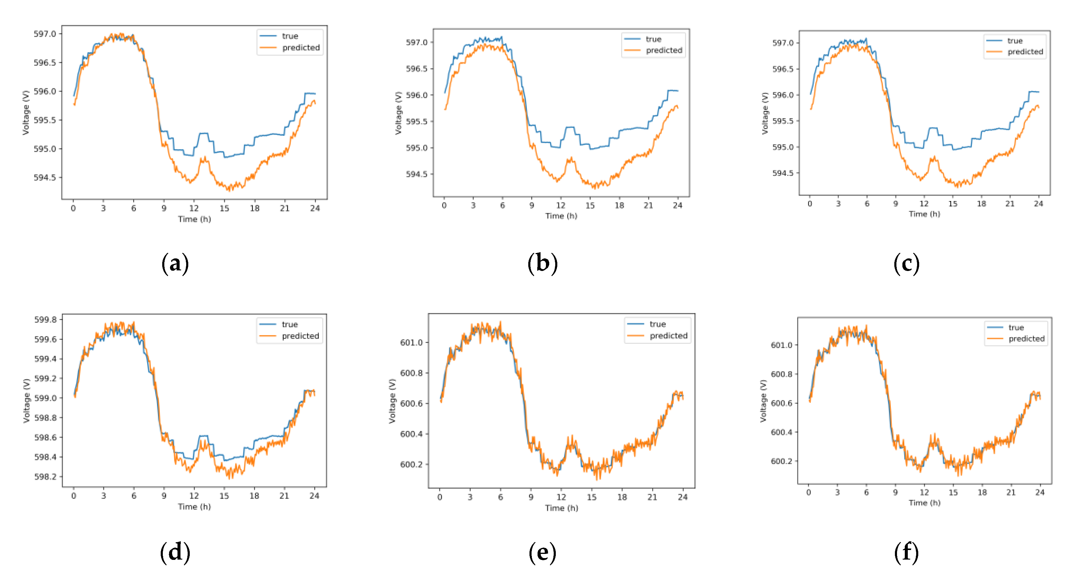
7. Discussion of Performance Evaluation

In order to demonstrate the effectiveness of the proposed method in estimating the DC microgrid’s state, the resulting error of the proposed modified LSTM-based state estimator is compared to the conventional WLS state estimator, the MLP-based state estimator, and the normal LSTM-based state estimator. Different types of evaluation metrics were calculated based on the equations (Equations (24–27)) shown in Section 5.4, specifically the MAE, MAPE, MSE, and RMSE. The values for each type of error are shown in

Table 2. Comparison of state estimator error values.

State Estimator	MAE	MAPE	MSE	RMSE
Conventional WLS	0.1862939	0.0312271	0.0757673	0.2752587
Modified LSTM-based	0.0673793	0.0112801	0.0088547	0.0940993
MLP-based	0.1156711	0.0193747	0.0217652	0.1475303
LSTM-based	0.0911940	0.0152753	0.0149962	0.1224592

.

Based on the results, the conventional WLS state estimator can be concluded to have the highest error rate for all error types compared to the deep-learning-based state estimators. This is due to the nature of the conventional WLS state estimator, which is dependent on the number of available measurements and the measurements’ error variance. The addition of pseudo-measurement in the conventional WLS state estimator did not help much in reducing the overall estimation error.

The difference between the conventional WLS state estimator and the deep-learning-based state estimators is the utilization of historical data and weight selection. Unlike the WLS state estimator, deep-learning-based state estimators also consider the past data information during their training process. Furthermore, in contrast to the WLS state estimator, for which weight is set based on the measurement error variance, the deep-learning-based state estimators can optimize their weight values to produce better predictions. By executing the learning approach and the data pattern recognition on the historical data, the deep-learning-based state estimators were shown to have smaller error values compared to the conventional WLS state estimator.

More specifically for the MLP approach, historical data were used in the training process of the network, resulting in an optimal weight to estimate the system state. The MLP network is trained using the backpropagation algorithm to learn the correlation between an output and current input, while optimizing its own weight with the gradient descent algorithm. As a result, the MLP-based state estimator produced better estimation than the conventional WLS state estimator.

Even though MLP can be used to make a time-series prediction, LSTM is much more suited for processing time-series data. Due to the structure of the network, LSTM allows all past information to persist over time. In the training process, the LSTM method calculated an output based on the current input and the previous output using the backpropagation through time algorithm, while the weight is optimized with the gradient descent algorithm. This process further improved the LSTM-based state estimator’s estimation more than the MLP-based and the conventional WLS state estimators.

The proposed modified LSTM-based state estimator has the smallest error value for all error types. Other than the advantages of the LSTM method itself, this is caused by the addition of the WLS loss function in the training of the LSTM network. Differing from the MSE loss function used in the normal LSTM-based state estimator, in the WLS loss function, the different weight values that were assigned to each parameter output error helped put an emphasis on the different types of measurements. The DC bus with the real simulated voltage measurement has the highest weight value, while the DC bus with pseudo-measurement has the lowest weight value. The addition of these weights further enhances the estimation output of the LSTM-based method.

The computation time of each state estimator is shown in

Table 3. Computation times of state estimators.

State Estimator	Computation Time
	Training (s)	Testing (s)
Conventional WLS	-	14.109
MLP-based	15.944	0.029
LSTM-based	42.586	0.169
Modified LSTM-based	51.092	0.157

. The training time is the computation time in the offline training stage for the deep-learning-based estimators, while the testing time is the computation time required for each state estimator to estimate the voltage magnitude of DC buses to its highest accuracy in the online testing stage. Based on the table, overall, it took longer for the conventional WLS state estimator to estimate the voltage magnitude of DC buses. For the deep-learning-based estimators, although the training processes took quite some time, the computation times in the online testing stage are significantly faster than the conventional WLS state estimator. The modified LSTM-based state estimator has the longest training time, followed by the normal LSTM-based state estimator and the MLP-based state estimator. Looking at the structure of the network, the LSTM network has a more complex structure compared to the MLP network. Consequently, the computation times for LSTM-based state estimators are longer than the MLP-based state estimator.

The implementation of the proposed state estimator as the deep learning method in the real power system might have some drawbacks. The deep-learning-based state estimator need to be trained with a lot of measurement data, as this is necessary for good approximation of the system and is generally not possible for bulk power systems. Additionally, for topology changes in the system, the learning process for SE needs to be repeated. However, for microgrids, the acquisition of measurement data is rather easy, as the metering technology has become more advanced. Consequently, this makes the modified LSTM-based SE more applicable for microgrids systems.

Overall, based on the analysis, in terms of accuracy and computation time, the proposed modified LSTM-based state estimator has the best results. This proves the superiority of the proposed method in estimating the DC microgrid’s state compared to the other state estimators tested in this paper.

8. Conclusions

The objective of the SE is to give accurate information of the state of a power system. With the proper information obtained from the SE, the system operator can operate and control the power system securely. The distribution system is an example of a section of the power system where real-time measurement is unfortunately lacking. The integration of DC microgrids in this system and the need for system control that comes with it intensify the urgency for a more accurate SE. In this paper, a new method for a DC microgrid’s SE is proposed. The state estimator is based on the deep learning method, which is the LSTM network. With LSTM as the deep learning method, the dependence on the error variance of measurement types for weight selection, such as in conventional WLS SE, was reduced, since the deep learning method can optimize its own weight. Furthermore, a specifically modified WLS loss function was integrated into the training process to assign certain weights for each measurement, which were used as inputs, based on their respective error variance. This novel method ensures more consistent accuracy in the estimation of all the bus voltages, irrespective of their distance to the voltage measurement point. The performance of the modified LSTM-based SE method and other previously investigated methods discussed in this paper was further validated by comparing the state estimators’ error value. Out of all state estimators, the modified LSTM-based state estimator is shown to have the lowest error value for all error types. Aside from increased accuracy, when compared to the conventional WLS state estimator, the deep-learning-based state estimators also give significantly faster computational time in the online testing stage after intensively training the network model in the offline training stage. Therefore, it can be concluded that with the adoption of the modified LSTM-based state estimator as the deep learning method, the estimation of the DC microgrid’s state can be performed more efficiently and with more accuracy compared to its predecessor.

References

1. Monticelli, A. Electric Power System State Estimation. Proc. IEEE 2000, 88, 262–282. [Google Scholar] [CrossRef]
2. Primadianto, A.; Lu, C. A Review on Distribution System State Estimation. IEEE Trans. Power Syst. 2017, 32, 3875–3883. [Google Scholar] [CrossRef]
3. Ahmad, F.; Rasool, A.; Ozsoy, E.; Rajasekar, S.; Sabanovic, A.; Elitas, M. Distribution system state estimation-A step towards smart grid. Renew. Sustain. Energy Rev. 2018, 81 Pt 2, 2659–2671. [Google Scholar] [CrossRef] [Green Version]
4. Zhu, K.; Nordstrom, L.; Ekstam, L. Application and analysis of optimum PMU placement methods with application to state estimation accuracy. In Proceedings of the IEEE Power Energy Society General Meeting, Calgary, AB, Canada, 26–30 July 2009; pp. 1–7. [Google Scholar]
5. Arritt, R.F.; Dugan, R.C. Distribution system analysis and the future smart grid. IEEE Trans. Ind. Appl. 2011, 47, 2343–2350. [Google Scholar] [CrossRef]
6. Kaushik, R.A.; Pindoriya, N.M. A hybrid AC-DC microgrid: Opportunities & key issues in implementation. In Proceedings of the International Conference on Green Computing and Electrical Engineering (ICGCCEE), Coimbatore, India, 6–8 March 2014. [Google Scholar]
7. Huang, Y.; Werner, S.; Huang, J.; Kashyap, N.; Gupta, V. State Estimation in Electric Power Grids: Meeting New Challenges Presented by the Requirements of the Future Grid. IEEE Signal Process. Mag. 2012, 29, 33–43. [Google Scholar] [CrossRef] [Green Version]
8. Hayes, B.; Prodanovic, M. State Estimation Techniques for Electric Power Distribution Systems. In Proceedings of the 2014 European Modelling Symposium, Pisa, Italy, 21–23 October 2014; pp. 303–308. [Google Scholar]
9. Hatziargyriou, N. Microgrids Architectures and Control; John Wiley and Sons Ltd.: West Sussex, UK, 2014. [Google Scholar]
10. McMenamin, J.S. Impact of AMI on Load Research and Forecasting. Available online: http://content.energycentral.com/reference/whitepapers/103036/Impact-of-AMI-on-Load-Research-and-Forecasting (accessed on 11 November 2019).
11. Krsman, V.; Tesanovic, B.; Dojic, J. Pre-processing of pseudo measurements based on AMI data for distribution system state estimation. In Proceedings of the Mediterranean Conference on Power Generation, Transmission, Distribution and Energy Conversion (MedPower 2016), Belgrade, Serbia, 6–9 November 2016; pp. 1–6. [Google Scholar]
12. Vaishnavi, C.; Sheikh, I.A. A Review of Power System State Estimation by Weighted Least Square Technique. In Proceedings of the National Conference on Recent Research in Engineering and Technology, Mogar-Anand, India, 13–14 March 2015; International Journal on Advance Engineering and Research Development (IJAERD): Gujarat, India, 2015. [Google Scholar]
13. Al-Othman, A.K. A fuzzy state estimator based on uncertain measurements. Measurement 2019, 42, 628–637. [Google Scholar] [CrossRef]
14. Xia, N.; Gooi, H.B.; Chen, S.; Hu, W. Decentralized State Estimation for Hybrid AC/DC Microgrids. IEEE Syst. J. 2019, 12, 434–443. [Google Scholar] [CrossRef]
15. Grahn, P.; Briggner, V.; Johansson, L.; Babazadeh, D.; Nordstrom, L.; Babazadeh, D. Centralized versus distributed state estimation for hybrid AC/HVDC grid. In Proceedings of the 2017 IEEE PES Innovative Smart Grid Technologies Conference Europe (ISGT-Europe), Torino, Italy, 26–29 September 2017; pp. 1–6. [Google Scholar]
16. Cosovic, M.; Vukobratovic, D. Fast real-time DC state estimation in electric power systems using belief propagation. In Proceedings of the 2017 IEEE International Conference on Smart Grid Communications (SmartGridComm), Dresden, Germany, 23–26 October 2017; pp. 207–212. [Google Scholar]
17. Abdel-Nasser, M.; Mahmoud, K.; Kashef, H. A Novel Smart Grid State Estimation Method based on Neural Networks. Int. J. Interact. Multimed. Artif. Intell. 2018, 5, 92–100. [Google Scholar] [CrossRef] [Green Version]
18. Zhang, L.; Wang, G.; Giannakis, G.B. Real-time Power System State Estimation and Forecasting via Deep Unrolled Neural Networks. IEEE Trans. Signal Process. 2018, 67, 4069–4077. [Google Scholar] [CrossRef] [Green Version]
19. Zamzam, A.S.; Fu, X.; Sidiropoulos, N.D. Data-driven Learning-based Optimization for Distribution System State Estimation. IEEE Trans. Power Syst. 2019, 34, 4796–4805. [Google Scholar] [CrossRef] [Green Version]
20. Barbeiro, P.N.P.; Krstulovic, J.; Teixeira, H.; Pereira, J.; Soares, F.J.; Iria, J.P. State estimation in distribution smart grids using autoencoders. In Proceedings of the 2014 IEEE 8th International Power Engineering and Optimization Conference (PEOCO2014), Langkawi, Malaysia, 24–25 March 2014; pp. 358–363. [Google Scholar]
21. Singh, A.; Tripathi, V.K. Load Forecasting using Multilayer Perceptron Neural Network. Int. J. Eng. Sci. Comput. 2016, 6. [Google Scholar] [CrossRef]
22. Kong, W.; Dong, Z.Y.; Jia, Y.; Hill, D.J.; Xu, Y.; Zhang, Y. Short-Term Residential Load Forecasting Based on LSTM Recurrent Neural Network. IEEE Trans. Smart Grid 2019, 10, 841–851. [Google Scholar] [CrossRef]
23. Husein, M.; Chung, I.-Y. Day-Ahead Solar Irradiance Forecasting for Microgrids Using a Long Short-Term Memory Recurrent Neural Network: A Deep Learning Approach. Energies 2019, 12, 1856. [Google Scholar] [CrossRef] [Green Version]
24. Pattayanak, S. Pro Deep Learning with Tensorflow; Apress: Berkeley, CA, USA, 2017. [Google Scholar]
25. Haykin, S. Neural Networks—A Comprehensive Foundation, 2nd ed.; Prentice-Hall: Englewood Cliffs, NJ, USA, 1998. [Google Scholar]
26. Goodfellow, I.; Bengio, Y.; Courville, A. Deep Learning; The MIT Press: Cambridge, MA, USA, 2016. [Google Scholar]
27. Kim, P. MATLAB Deep Learning; Apress: Berkeley, CA, USA, 2017. [Google Scholar]
28. Nwankpa, C.; Ijomah, W.; Gachagan, A.; Marshall, S. Activation functions: Comparison of trends in practice and research for deep learning. arXiv 2018, arXiv:1811.03378. [Google Scholar]
29. Rumelhart, D.; Hinton, G.; Williams, R. Learning representations by back-propagating errors. Nature 1986, 323, 533–536. [Google Scholar] [CrossRef]
30. Hochreiter, S.; Schmidhuber, J. Long short-term memory. Neural Comput. 1997, 9, 1735–1780. [Google Scholar] [CrossRef]
Figure 1. A perceptron.
Applsci 10 03028 g001
Figure 2. A multilayer perceptron (MLP) network.
Applsci 10 03028 g002
Figure 3. A single long short-term memory (LSTM) unit.
Applsci 10 03028 g003
Figure 4. Configuration of a DC microgrid system.
Applsci 10 03028 g004
Figure 5. Conventional weighted least squares (WLS) voltage estimation results for: (a) bus 1; (b) bus 2; (c) bus 3; (d) bus 4; (e) bus 5; (f) bus 6; (g) bus 7; (h) bus 8; (i) bus 9.
Applsci 10 03028 g005aApplsci 10 03028 g005b
Figure 6. Modified LSTM-based voltage estimation results for: (a) bus 1; (b) bus 2; (c) bus 3; (d) bus 4; (e) bus 5; (f) bus 6; (g) bus 7; (h) bus 8; (i) bus 9.
Applsci 10 03028 g006aApplsci 10 03028 g006b