A Novel Hydraulic Fracturing Method Based on the Coupled CFD-DEM Numerical Simulation Study

Featured Application

Based on a coupled CFD-DEM numerical simulation and an experimental study, a novel hydraulic fracturing method for the development of tight reservoirs is proposed.

Abstract

For the development of tight oil reservoirs, hydraulic fracturing employing variable fluid viscosity and proppant density is essential for addressing the problems of uneven placement of proppants in fractures and low propping efficiency. However, the influence mechanisms of fracturing fluid viscosity and proppant density on proppant transport in fractures remain unclear. Based on computational fluid dynamics (CFD) and the discrete element method (DEM), a proppant transport model with fluid–particle two-phase coupling is established in this study. In addition, a novel large-scale visual fracture simulation device was developed to realize the online visual monitoring of proppant transport, and a proppant transport experiment under the condition of variable viscosity fracturing fluid and proppant density was conducted. By comparing the experimental results and the numerical simulation results, the accuracy of the proppant transport numerical model was verified. Subsequently, through a proppant transport numerical simulation, the effects of fracturing fluid viscosity and proppant density on proppant transport were analyzed. The results show that as the viscosity of the fracturing fluid increases, the length of the “no proppant zone” at the front end of the fracture increases, and proppant particles can be transported further. When alternately injecting fracturing fluids of different viscosities, the viscosity ratio of the fracturing fluids should be adjusted between 2 and 5 to form optimal proppant placement. During the process of variable proppant density fracturing, when high-density proppant was pumped after low-density proppant, proppants of different densities laid fractures evenly and vertically. Conversely, when low-density proppant was pumped after high-density proppant, the low-density proppant could be transported farther into the fracture to form a longer sandbank. Based on the abovementioned observations, a novel hydraulic fracturing method is proposed to optimize the placement of proppants in fractures by adjusting the fracturing fluid viscosity and proppant density. This method has been successfully applied to more than 10 oil wells of the Bohai Bay Basin in Eastern China, and the average daily oil production per well increased by 7.4 t, significantly improving the functioning of fracturing. The proppant settlement and transport laws of proppant in fractures during variable viscosity and density fracturing can be efficiently revealed through a visualized proppant transport experiment and numerical simulation study. The novel fracturing method proposed in this study can significantly improve the hydraulic fracturing effect in tight oil reservoirs.

1. Introduction

Hydraulic fracturing with variable fluid viscosity and proppant density is critical for the development of tight oil and gas reservoirs. This type of fracturing adjusts the viscosity of the fracturing fluid and the proppant density to improve the proppant placement in fractures, which determines the final effect of fracturing measures [1,2,3,4]. The proppant transport law in fractures is essential in affecting the morphology of proppant placement in fractures [5,6,7]. The flow state of the fluid in its fractures, the properties of the fracturing fluid and proppant, and the interaction between the proppant particles all seriously affect proppant transport and sedimentation [8,9,10].

Researchers at home and abroad have conducted a significant amount of research on the proppant transport law via experimental tests and numerical simulation methods [11,12]. Kern et al. [13] conducted the first vertical fracture experiment, injecting water and sand at a constant rate. Shokir et al. [14] established a small-slit experimental device to study the effect of proppant concentration on proppant convection. Dayan et al. [15] established a small fracture device with branch fractures and studied the proppant transport behavior in complex fractures. The results show that if the flow velocity is low, then the proppant only accumulates in the main fracture. When the flow velocity is greater than a specified threshold, the proppant can enter the secondary fracture from the main fracture. Sahai [16] carried out large-scale experimental tests in the laboratory to evaluate proppant transport in complex fracture geometries with primary and secondary fracture slots. Chun et al. [17] found through experiments that as the fracture plane angle becomes closer to the horizontal plane, the proppant withstands greater friction along the wall, and the proppant placement area is larger.

Several numerical simulation studies focused on the proppant transport mechanism have been conducted. Babcock et al. [18] took the lead in developing correlations using the “equilibrium velocity” and “bank-buildup constant”, which can predict the proppant settling in both Newtonian and non-Newtonian fluids. Gadde et al. [19] established a proppant transport model, coupled it with a three-dimensional fracture propagation model, and solved the model using the finite element method. Their results show that the proppant settlement has a significant effect on the length of a fracture, considering turbulent flow. Huang et al. [20] used the mixture model to simulate the movement of proppants carried by high viscosity fracturing fluids in simple rectangular fractures. Zhang et al. [21] established a Euler–Euler dual-fluid model of fluid-structure coupling that simulated the behavior of proppant transported by water in a single slot, and studied the effects of parameters such as the perforation position and injection speed on the shape of the proppant dune. Zeng et al. [22] adopted a representative particle model (RPM) to scale up proppant particles to study the transport mechanism of proppants in fractures. Yang et al. [23] simplified the shale complex fracture network into a complex fracture model in which the primary and secondary fractures are orthogonal to each other. Kou et al. [24] used the CFD-DEM method to study proppant transport in complex fractures, indicating that the proppant concentration and the ratio between the secondary fracture aperture and proppant diameter are the key factors affecting the proppant transport during fracture interactions. However, very few studies have focused on the effects of fracturing fluid viscosity and proppant density on the proppant transport law.

Based on computational fluid dynamics and the discrete element method, the effects of proppant and proppant, proppant and fluid, and proppant and fracture wall surfaces are considered to establish a fluid–particle coupled proppant transport model. Through a numerical simulation of proppant transport, the effects of the fracturing fluid viscosity and proppant density on the proppant transport law were analyzed. In this study, the proppant transport law in fractures during the process of hydraulic fracturing with variable fluid viscosity and proppant density is effectively revealed. This is used as a basis for theoretical research of the proppant transport law and parameter optimization of hydraulic fracturing with variable fluid viscosity and proppant density.

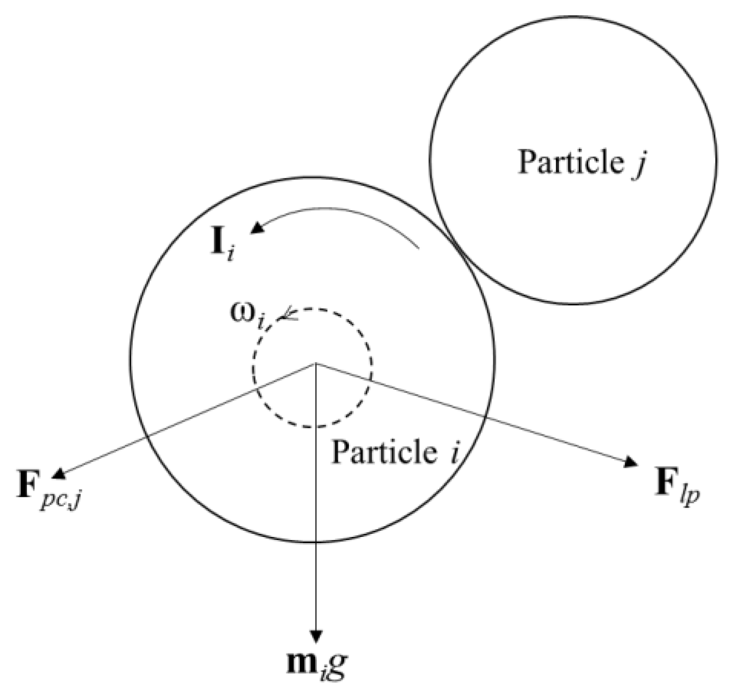
2. Proppant Transport Model

In this study, a coupled method of CFD and DEM is utilized. A fluid–particle two-phase flow model is established by considering particle–particle, particle–wall, and fluid–particle interaction forces. The following assumptions were made for the model.

• The fluid (slippery water) is incompressible, and the fluid rheology and temperature will not change during the simulation.
• Ultralow density proppants are regular spherical particles.
• The particles were fully mixed with the fluid, and the particles were evenly distributed in the fluid at the fracture entrance.
• The particles are rigid bodies, the spheres are not deformed, and the contact between the particles is point contact.

When establishing the governing equation of the fluid, the effect of particles on fluid is considered. Therefore, the liquid flow control equation is the Navier–Stokes equation of liquid–solid coupling. Because the simulated fluid inlet velocity is high and the flow field changes drastically, after calculating the Reynolds number, the standard $\mathrm{k}-\epsilon$ model is invoked as the turbulent flow model to solve the slurry flow field [25,26,27,28].

The turbulence flow energy equation is as follows:

$$\frac{\partial (\rho k)}{\partial t}+\frac{\partial (\rho k{u}_i)}{\partial x_i}=\frac{\partial }{\partial x_j}\left[\left(\mu +\frac{{\mu }_t}{{\sigma }_k}\right)\frac{\partial k}{\partial x_j}\right]+G_k-\beta \epsilon +S_K$$

(1)

The turbulence diffusion equation is as follows:

$$\frac{\partial (\rho \epsilon )}{\partial t}+\frac{\partial (\rho \epsilon u_i)}{\partial x_i}=\frac{\partial }{\partial x_j}\left[\left(\mu +\frac{{\mu }_t}{{\sigma }_{\epsilon }}\right)\frac{\partial \epsilon }{\partial x_j}\right]+\frac{C_{1\epsilon }}{k}{G}_k-C_{2\epsilon }\rho \frac{{\epsilon }^2}{k}+S_{\epsilon }$$

(2)

where $k$ is the turbulence kinetic energy of the fluid phase; $\epsilon$ is the turbulence dissipation rate; $G_k$ is the turbulence kinetic energy generation term; ${\sigma }_k$ is the Prandtl number corresponding to the turbulence kinetic energy, which is 1.0; ${\sigma }_{\epsilon }$ is the Prandtl number corresponding to the turbulence dissipation rate, and the value is taken as 1.3; $S_K$ and $S_{\epsilon }$ are the turbulence exchange term between the liquid and solid phases, respectively; and $C_{1\epsilon }$ and $C_{2\epsilon }$ are constants with values of 1.44 and 1.92, respectively.

${\mu }_t$ is the turbulence viscosity and its expression is as follows:

$${\mu }_t=\rho C_{\mu }\frac{k^2}{\epsilon }$$

(3)

The motion of proppant particles follows Newton’s second law. When particles follow the fluid, the movement of each particle is affected by the surrounding fluid and adjacent particles; hence, the particles are mainly subject to the force from the fluid, adjacent particles and fracture walls (Figure 1).

The equation of particle motion consists of a translational equation and a rotational equation, following Newton’s second law of motion. The equation of the translational is as follows:

$$m_{p,i}\frac{\mathrm{d}{u}_{p,i}}{\mathrm{d}t}={\displaystyle \sum F_{pc,ij}}+F_{lp,i}+m_{p,i}g$$

(4)

The rotation equation is as follows:

$$I_{pc,ij}\frac{\mathrm{d}{\omega }_{p,i}}{\mathrm{d}t}=T_{pc,ij}$$

(5)

where $m_i$ is the mass of particle i, $u_{p,i}$ is the linear velocity of the particle, $F_{pc,ij}$ is the contact force produced by particle i in contact with other particles, $F_{lp,i}$ is the force of the fluid on particle i, $I_{pc,ij}$ is the moment of inertia of particle i, ${\omega }_{p,i}$ is the angular velocity of particle i, and $T_{pc,ij}$ is the contact moment produced by particle i in contact with particle j.

Fluid–solid coupling requires the establishment of a fluid–particle interaction model and a particle–particle interaction model. The buoyancy and drag forces of the fluid on the particles are mainly considered in the fluid–particle force model. By calculating the particle Reynolds number, the drag force is obtained using the Gidspow model [29]. The calculation formula is as follows:

$$F_{l\mathrm{s}}=\{\begin{array}{cc}\frac{3}{4}{C}_D\frac{{\rho }_l\left(1-{\epsilon }_s\right){\epsilon }_s\left|{\overrightarrow{u}}_s-{\overrightarrow{u}}_l\right|}{d_s}{\left(1-{\epsilon }_s\right)}^{-2.65}& {\epsilon }_l>0.8\\ \frac{150{\epsilon }_s{}^2{\mu }_l}{\left(1-{\epsilon }_s\right)d_s^2}+\frac{1.75{\rho }_l{\epsilon }_s\left|{\overrightarrow{u}}_s-{\overrightarrow{u}}_l\right|}{d_s}& {\epsilon }_l\le 0.8\end{array}$$

(6)

$$C_D=\frac{24}{{\epsilon }_l{\mathrm{Re}}_s}\left(1+0.15{\left({\epsilon }_l{\mathrm{Re}}_s\right)}^{0.687}\right)$$

(7)

$${\mathrm{Re}}_{\mathrm{s}}=\frac{{\epsilon }_l{\rho }_l\left|u_s-u_l\right|d_s}{{\mu }_l}$$

(8)

where ${\rho }_l$ is the density of the liquid, ${\epsilon }_s$ is the volume fraction of the particles, ${\overrightarrow{u}}_s$ is the moving speed of the particles, ${\overrightarrow{u}}_l$ is the moving speed of the liquid phase, $d_s$ is the particle size of the particle phase, and ${\mu }_l$ is the fluid viscosity.

When particle i migrates in the fracture, it receives contact force from particle j and noncontact force from particle k. As the particle size of this article is small, only the contact force between particles and particles is considered. When fracturing fluid flows in a fracture, its boundary conditions include inlet conditions and wall conditions. The inlet conditions were set as a constant speed, and the outlet conditions used a pressure of 0 MPa. The fracture wall surface was set to have no slip boundary; that is, the normal velocity and tangential velocity of the fluid at the wall surface were both zero. In the fracturing process, prefluid is first injected into the formation to open the fracture, and then uniformly mixed slurry is injected. In order to accurately simulate this process, the stable flow is first calculated to converge in CFD, and stable flow field is used as the initial condition.

Based on the abovementioned two–phase coupling model, a fracture physical model (4000 mm × 600 mm × 6 mm) was established. As the fracture model has a simple shape and is a rectangular fracture, according to the previous research experience, the mesh refinement was performed at the inlet and exit of the fracture model, a hexahedron was used to mesh the fracture model. Two hundred, 30 and 4 grids were divided in sequence along the length, height and width of the fracture, with a total grid number of 24,000. Based on the Rayleigh time step calculation results, the proppant particle simulation time step was set to 0.2 times the Rayleigh time step, which is 2 × 10⁻⁵ s, and the fluid simulation time step was set to 20 times the Rayleigh time step, which is 2 × 10⁻³ s. The specific steps in the CFD–DEM coupling solution are as follows:

• CFD iteratively calculates the fluid flow field distribution and the fluid–particle interaction force according to the initial conditions, and transmits information such as drag and buoyancy to the DEM solver.
• The DEM solver calculates the contact force of each particle, including the particle–particle and particle–wall forces, and updates the particle position and velocity according to the combined force. The volume fraction and the force of the particles on the fluid were calculated and passed to the CFD solver.
• Based on the updated particle volume fraction and the force between the two phases, the CFD solver starts the iterative solution of the next time step, repeating the processes of (1) and (2) until convergence or reaching a preset number of simulation steps.

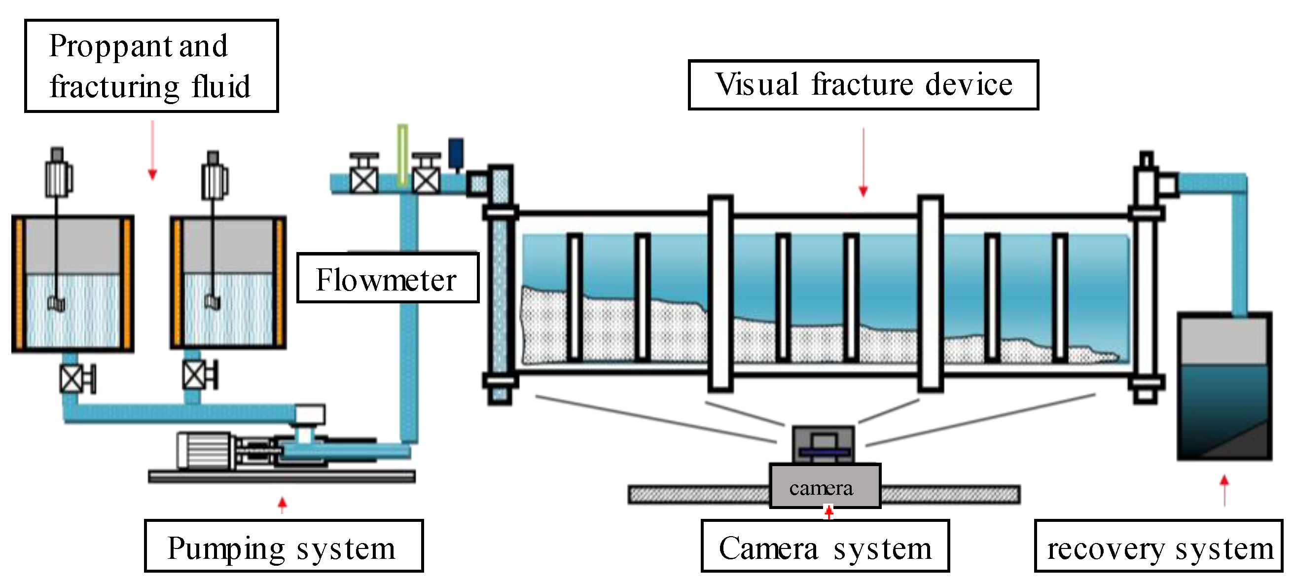
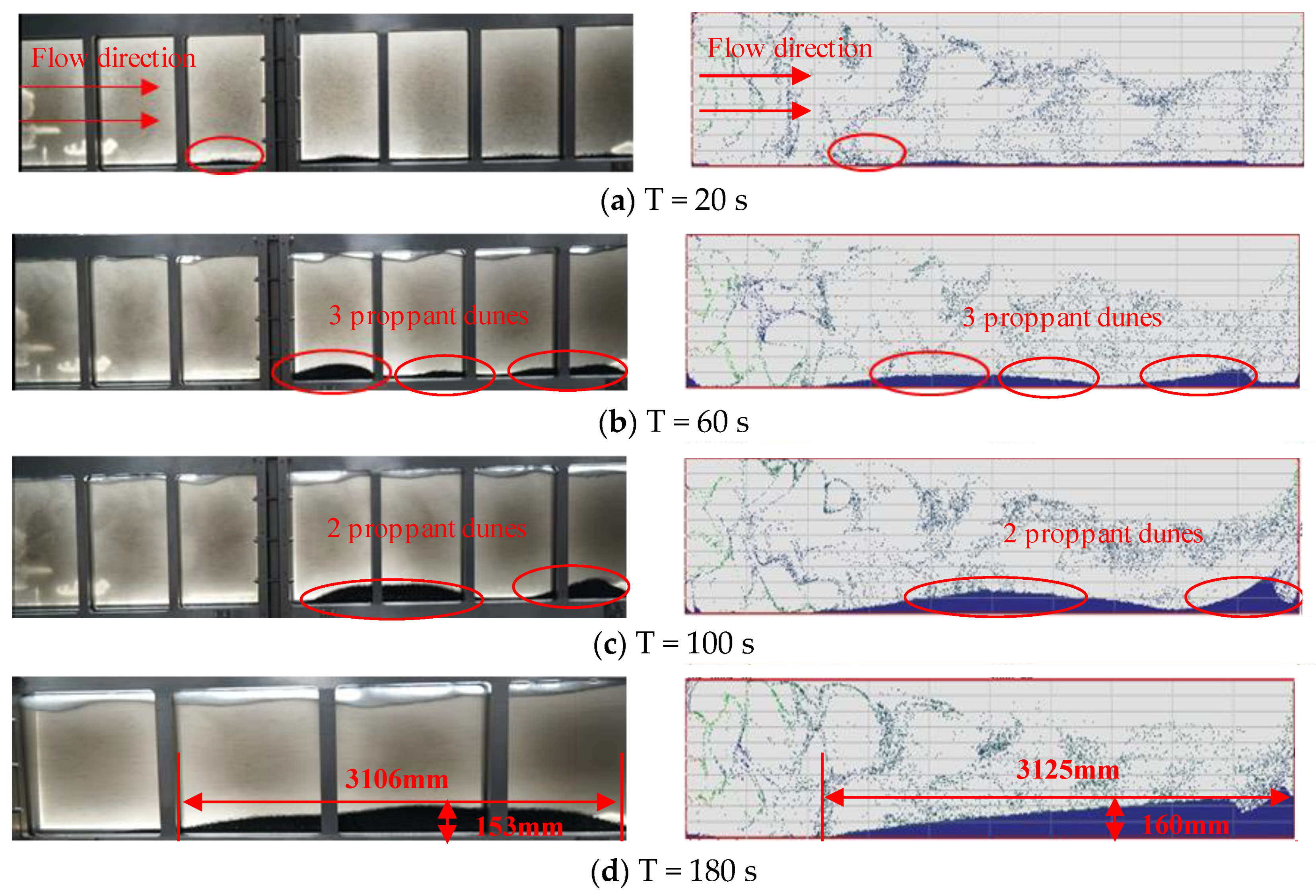
3. Experimental Verification

To further verify the reliability of the two-phase coupling model, an experiment on the proppant transport in visualized fractures was conducted. The experimental device consisted of six main parts (Figure 2). The experimental steps were as follows:

• Prepare the proper amount of proppant and fracturing fluid with different viscosities.
• The proppant and the fracturing fluid are thoroughly mixed by a mixing system.
• The mixed slurry is pumped to the visual fracture system through the pumping device.
• Collect the proppant placement morphology in the fracture device at different times through the camera system.
• Waste treatment and recycling.

Through physical experiments and numerical simulations, the flow of proppant in the fracturing fluid (slip water) was studied. In order to truly reflect the flow behavior of proppant particles in fractures, it is necessary to ensure that the dynamic behavior of the slurry in the numerical simulation is similar to that in physics experiments. Therefore, based on the principle of equal linear speed, the oilfield pumping rate wasw converted into the experimental pumping rate and the inlet speed of the numerical simulation. The conversion formula is as follows:

$$v_1=\frac{v_2}{h_2\times w_2\times 2}\times \left(h_1\times w_1\right)\times 1000$$

(9)

where $v_1$ is the experimental pumping rate, $v_2$ is the oilfield pumping rate, $h_1$ is the experimental fracture height, $h_2$ is the oilfield fracture height, $w_1$ is the experimental fracture width, and $w_2$ is the oilfield fracture width.

The experimental parameters are listed in

Table 1. Experimental and numerical simulation parameters.

Oilfield Pumping Rate (m3/min)	Experimental Pumping Rate (L/min)	Simulation Inlet Speed (m/s)	Proppant Concentration (%)
10	195	0.93	2
Proppant diameter (mm)	Proppant density (kg/m3)	Fluid viscosity (mPa·s)	Fluid density (kg/m3)
1	1350	3	998

.

To verify the accuracy of this fluid–particle two–phase coupled flow model, the simulation results at different times were compared with the experimental results (Figure 3). Owing to the influence of perforation, the flow velocity of the fluid near the fracture inlet is high and changes rapidly, and the proppant hardly settles down.

4. Factors Influencing Proppant Transportation

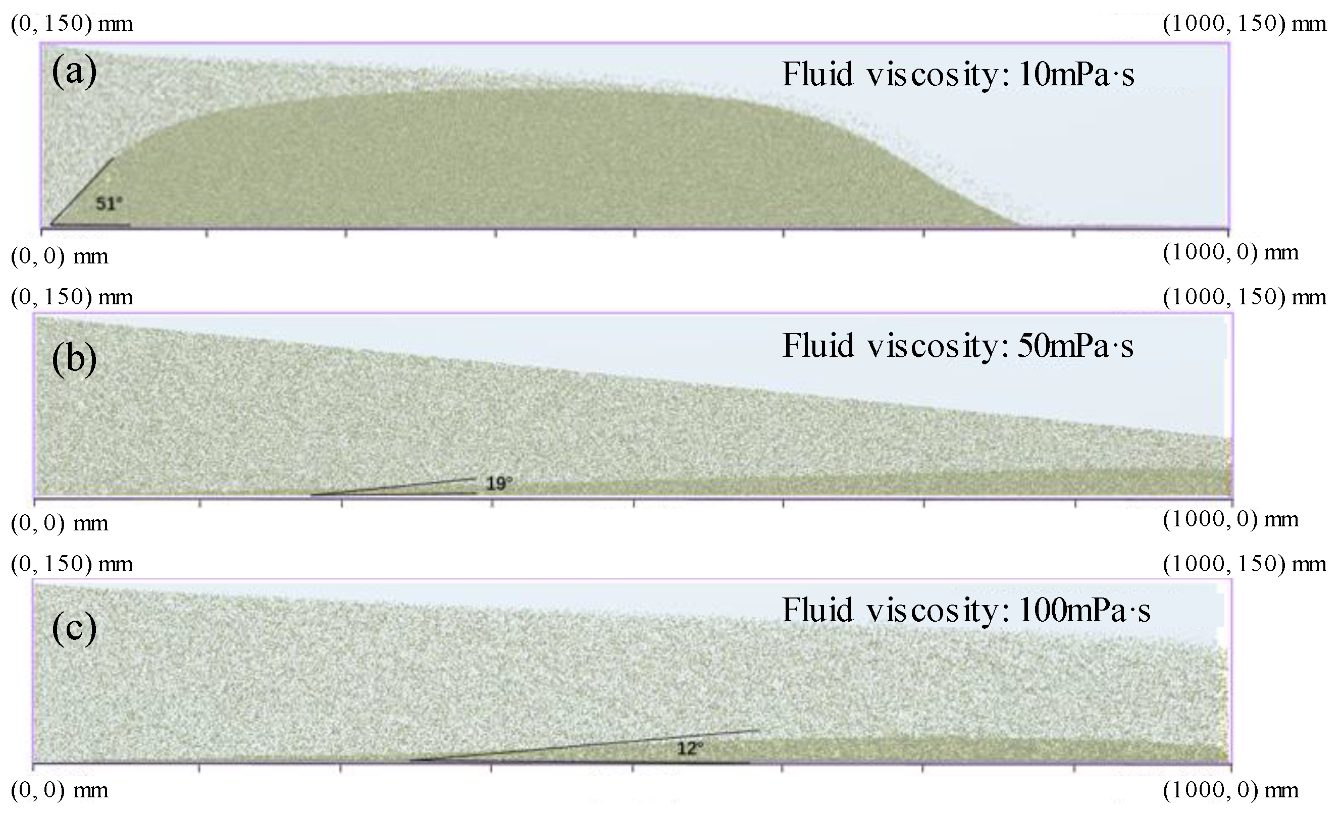
4.1. Fracturing Fluid Viscosity

In this study, three different fluid viscosities of 10, 50, and 100 mPa·s were selected to study the effect of fracturing fluid viscosity on proppant transport. The results are presented in Figure 4.

From an analysis of the sand bank accumulation position, there is an evident “sand-free area” at the entrance of the crack. When the fracturing fluid viscosity increased from 10 to 50 mPa·s, the distance between the sand bank and the fracture entrance increased from 10 to 312 mm. When the fracturing fluid viscosity increased to 100 mPa·s, the distance between the sand bank and inlet increased to 374 mm. The greater the viscosity of the fracturing fluid, the longer the “sand-free area.” The sand dune accumulation position obviously moves toward the fracture end, and more proppant is moved far away from the fracture.

From an analysis of the sand bank morphology, when the fracturing fluid viscosity increased from 10 to 50 mPa·s, the height of the sand dune decreased from 115 to 30 mm, and the “inlet slope angle” decreased from 51° to 19°. When the viscosity of the fracturing fluid increased to 100 mPa·s, the height of the dune decreased to 20 mm, and the “inlet slope angle” decreased to 12°. When the fracturing fluid has a low viscosity, proppant particles mainly settle at the fracture entrance. As the viscosity of the fracturing fluid increases, the suspending force of the fracturing fluid on the proppant increases, and the proppant particles can be transported to further positions inside the fracture, which can obtain a longer dune length, but the dune height decreases.

It is concluded that when a low viscosity fracturing fluid is injected, the proppant transport distance is short, and a short sand-bank length is obtained. When a high-viscosity fracturing fluid is injected, the “sand-free zone” at the fracture entrance is longer, and the sand bank height is lower. Therefore, injecting only one fracturing fluid of the same viscosity does not contribute to improving the effectiveness of proppant placement.

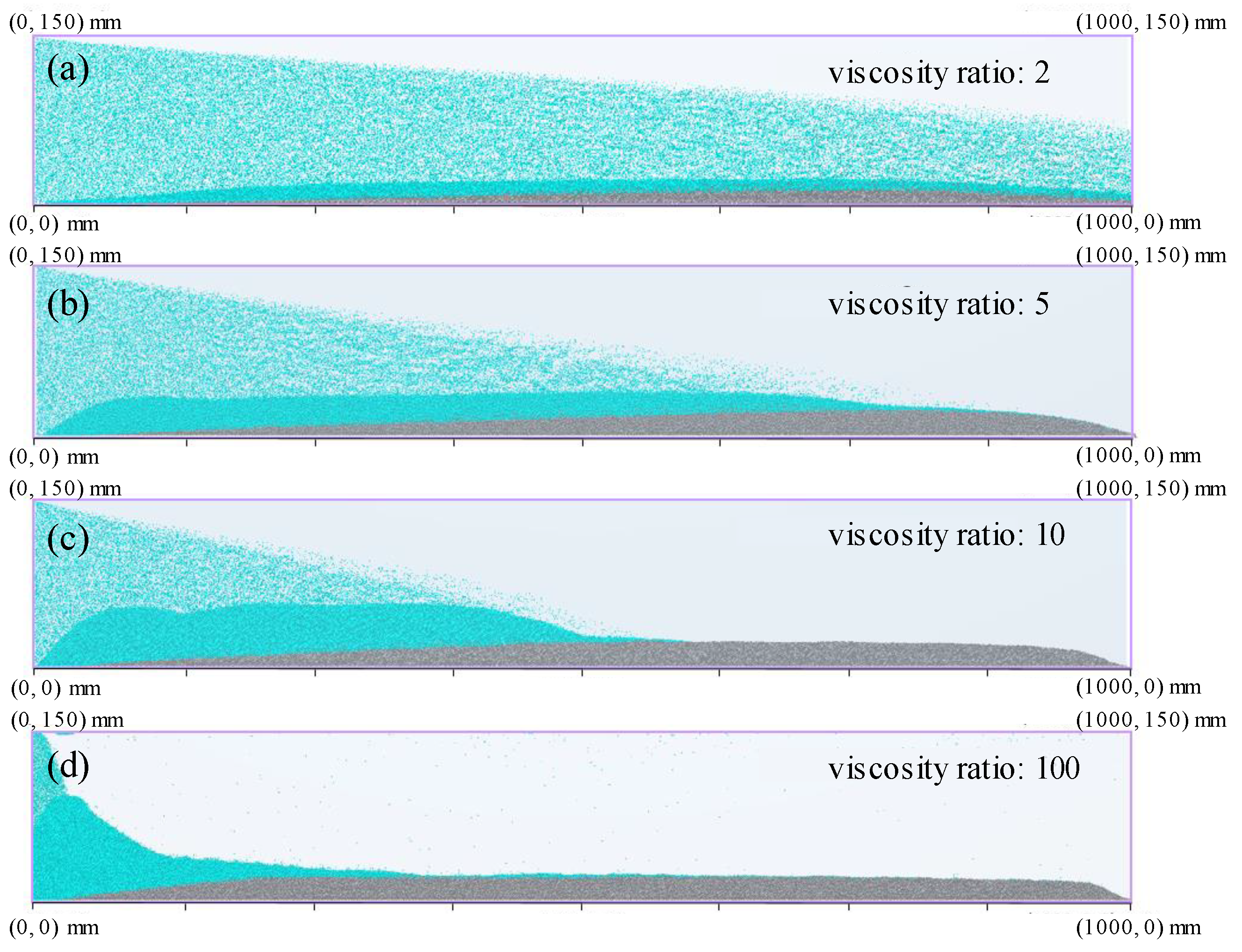
4.2. Fracturing Fluid Viscosity Ratio

In this study, four different fracturing fluid viscosity ratios of 100, 10, 5, and 2 were selected to study the effect of the viscosity ratio on proppant transport and proppant placement. Fracturing fluid is injected with a viscosity of 100 mPa·s, and then fracturing fluid with a lower viscosity is injected.

Under different viscosity ratio conditions, the shape of the sand dunes is significantly altered (Figure 5). Comparing the lengths of sand dunes under different viscosity ratios, it was found that when the viscosity ratio was greater than or equal to 5, the length of the sand banks was equal to 1000 mm, and the length of the sand banks did not increase after lower viscosity fracturing fluid was injected. When the viscosity ratio was 2, because the fracturing fluid injected later still had a good carrying capacity, the length of the sand dune increased (to greater than 1000 mm). With regard to the height of the sand bank, when the viscosity ratio increased from 2 to 5, the height of the sand bank increased from 29 to 40 mm. In the case of viscosity ratios of 10 and 100, although the sand dune height increased dramatically, its height increase mainly occurred at the fracture inlet, and the proppant was unevenly distributed in the fracture. In particular, when the viscosity ratio was increased to 100, the proppant settled in the fracture inlet almost as soon as it entered the fracture, increasing the risk of sand plugging.

When the variable viscosity injection method was used, the viscosity ratio increased within a certain range, the proppant transport distance increased, the height of the sand bank was higher, and the proppant was more uniformly laid. Therefore, to form an effective proppant placement shape, the viscosity ratio should be maintained between 2 and 5.

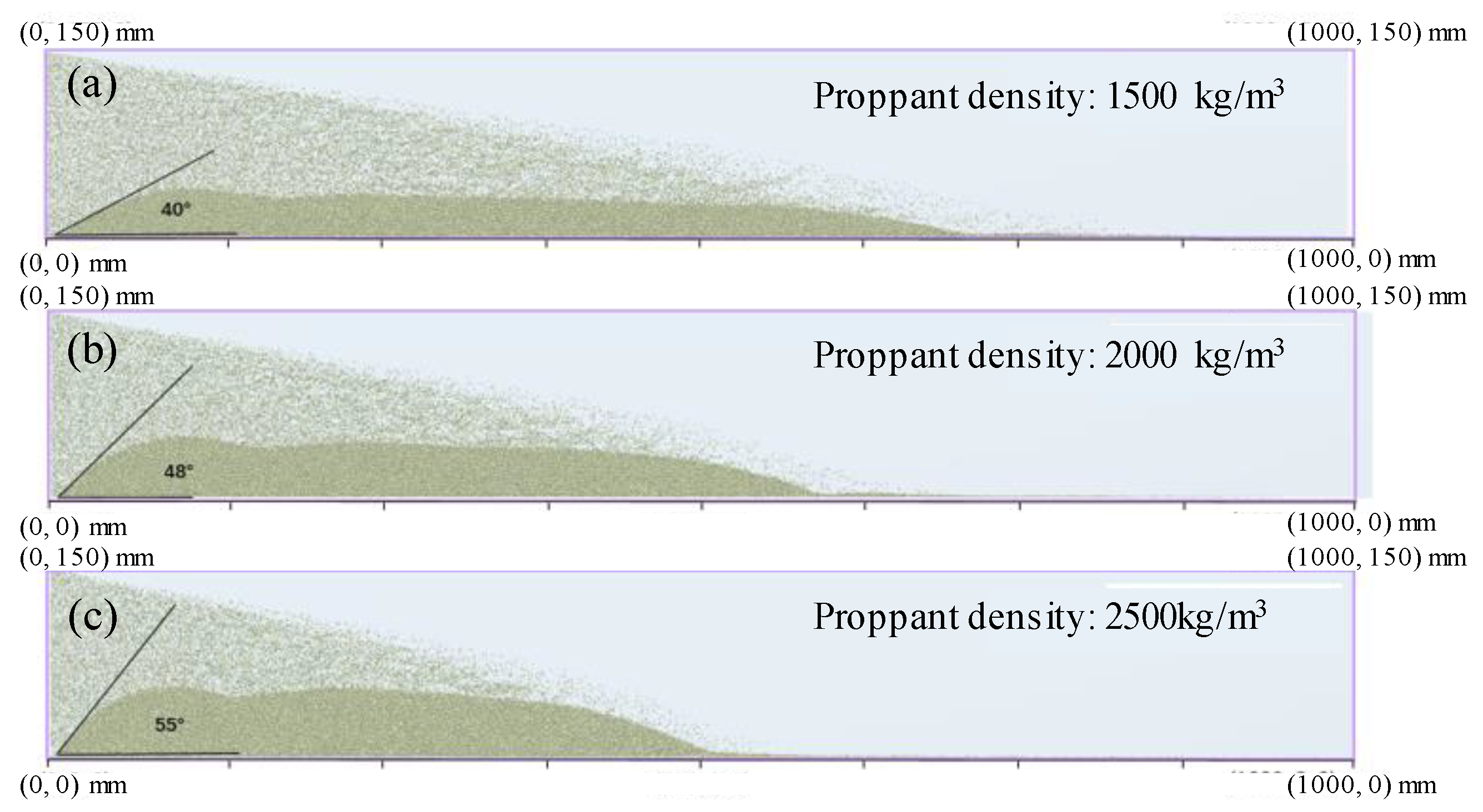
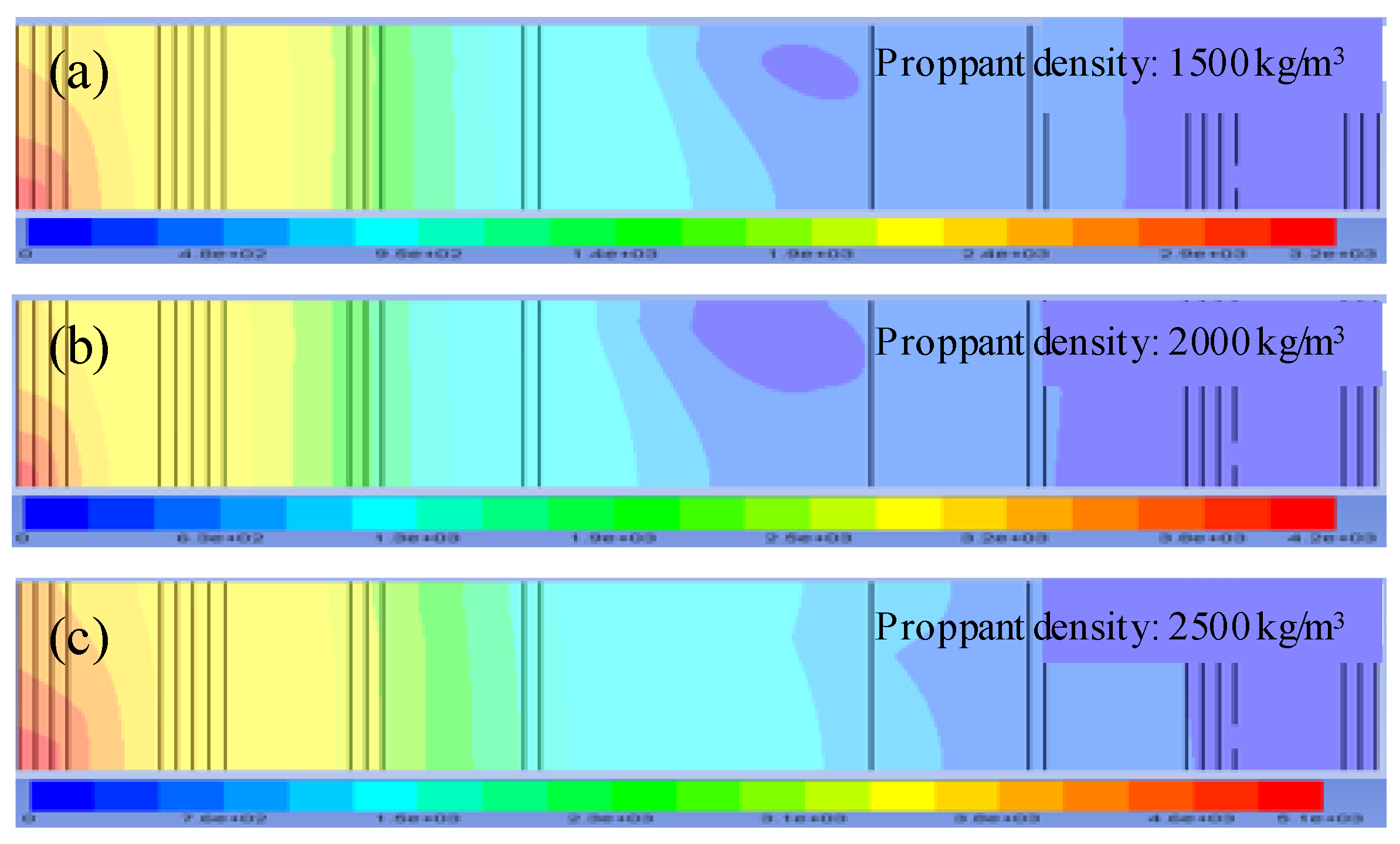
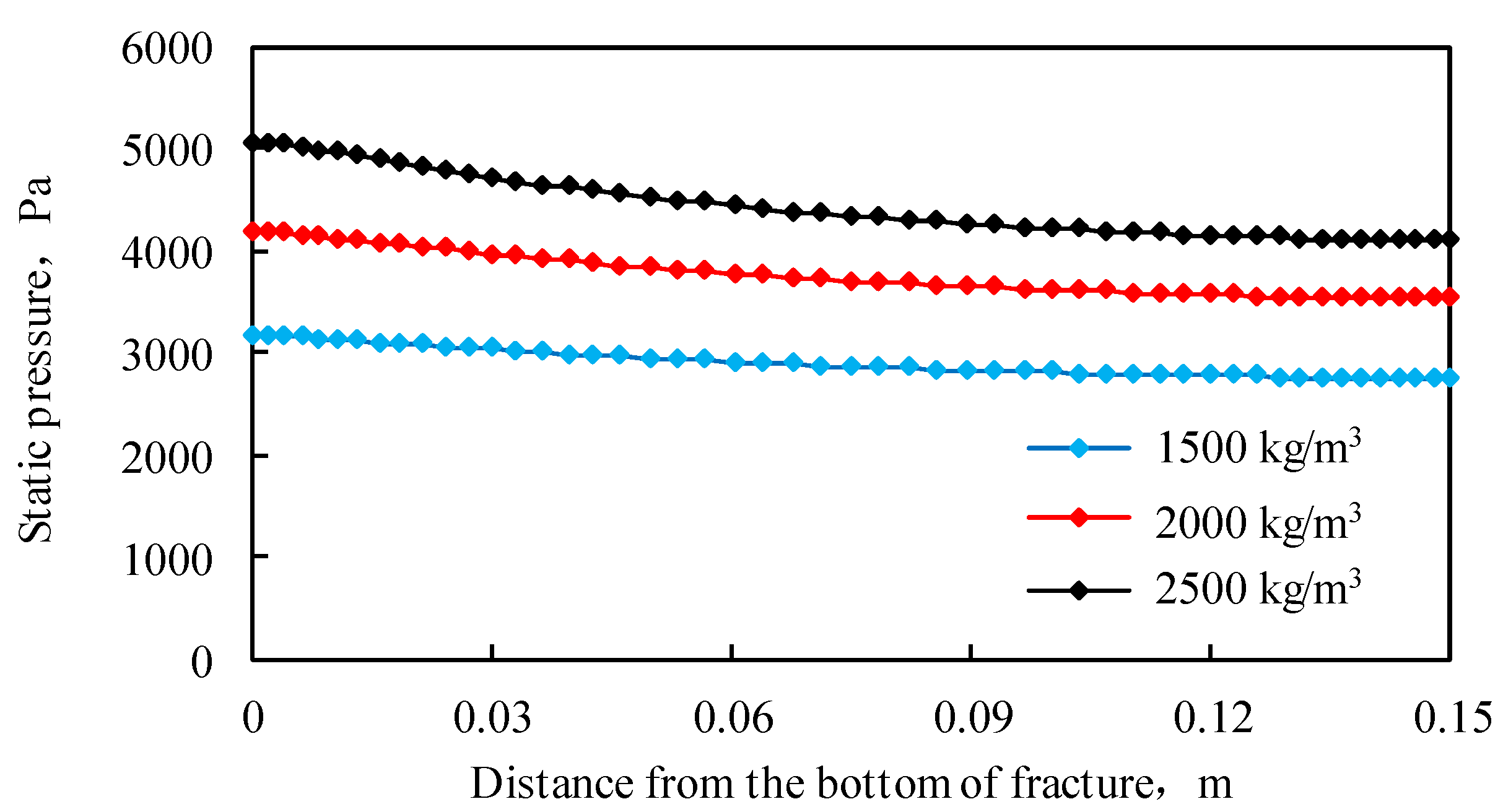
4.3. Proppant Density

In this study, three different proppants densities of 1500, 2000, and 2500 kg/m³ were selected for the numerical simulation, to study the effect of proppant density on proppant transport and sand bank placement.

As shown in Figure 6, from the perspective of the sand bank shape, the sand dune shape has a two-stage “stepped shape.” When the proppant density increased from 1500 to 2000 kg/m³, the length of the sand dune decreased from 692 to 575 mm, and the “inlet slope angle” increased from 40° to 48°. When the proppant density increased to 2500 kg/m³, the dune length decreased to 518 mm and the “inlet slope angle” of the dune increased to 55°. As the proppant density increased, the height of the sand bank increased, the length of the sand dune decreased, and the proppant tended to accumulate at the fracture inlet.

Figure 7 shows the distribution of static pressure in fractures under different proppant densities. It can be seen from the figure that the pressure in the fracture gradually decreases upward along the height of the fracture, and the pressure at the bottom of the fracture inlet is the highest. Figure 8 shows the pressure distribution at 2 mm from the fracture inlet. When the proppant density increased from 1500 to 2500 kg/m³, the maximum static pressure at the fracture inlet increased from 3000 to 5000 Pa. This may make it difficult for the proppant to enter the fracture, and proppant blockage may occur.

It is possible to conclude that a lower sand dune height is obtained when the low-density proppant is injected. When injecting a high-density proppant, the proppant has a tendency to settle and accumulate at the fracture inlet, which may cause the proppant to block the fracture inlet. Therefore, injecting only one proppant of the same density does not contribute to improve the effectiveness of proppant placement.

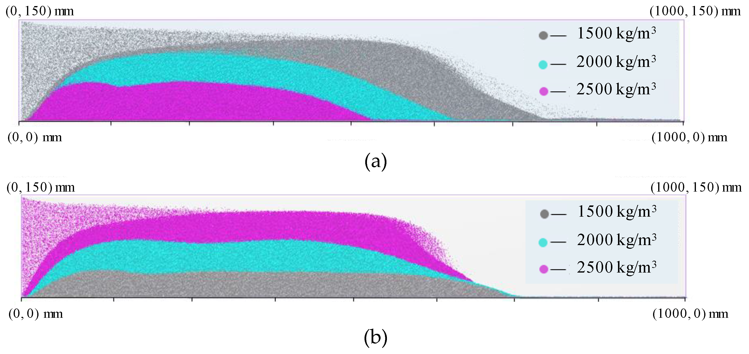
4.4. Variable Proppant Density

In this study, three proppant densities—1500, 2000, and 2500 kg/m³—were selected. By changing the order in which the three proppants were injected into the fracture with the fracturing fluid, proppant placement under different injection orders was studied.

As shown in Figure 9a, from the perspective of sand dune morphology, first pumping high-density proppant formed “short and high” sand dunes at the fracture inlet, resulting in an increased fracture inlet pressure. It is difficult to pump the low-density proppant in the latter stage, which may cause the proppant to block the fracture inlet. As shown in Figure 9b, the low-density proppant is pumped first, and the proppant can be transported to the far side of the fracture to form a “long and short” dune. Then, a high-density proppant was injected. This settled and accumulated at the fracture inlet, filling the “sand-free zone” formed in the initial stage. High-density proppants continued to accumulate on low-density dunes, increasing the height of the dunes. Therefore, the second method of injecting the variable-density proppant is beneficial for obtaining a more effective proppant placement.

5. Novel Hydraulic Fracturing Method

Based on the results of the above numerical simulation, a new variable-viscosity and variable-density fracturing method was proposed for tight oil and gas reservoirs. The morphology of proppants in fractures was optimized by precisely controlling the viscosity of the fracturing fluid and proppant density. The method includes the following two steps:

• Pumping high-viscosity fracturing fluid and low-density proppant

First, high-viscosity fracturing fluid and low-density proppant are pumped into the fracture. The low-density proppant is carried to the far side of the fracture, increasing the distance of proppant placement and the effective fracture stimulation area. Simultaneously, the accumulation of proppant at the fracture inlet is reduced, static pressure at the fracture inlet is reduced, and the risk of proppant clogging is decreased.

• Pumping low-viscosity fracturing fluid and high-density proppant

Then, low-viscosity fracturing fluid and high-density proppant are pumped into the fracture while ensuring that the viscosity ratio of the fracturing fluid is between 2 and 5. The high-density large-diameter proppant settles and accumulates at the fracture inlet, filling the “sand-free zone” formed in the initial stage, and forming fractures with high conductivity in the near-well zone. At the same time, high-density proppants continue to accumulate on low-density proppant dunes, increasing the height of the proppant dunes and forming an effective proppant placement, thus effectively improving the reservoir.

According to statistics, the method has been successfully applied to more than 10 oil wells of the Bohai Bay Basin in eastern China, and the average daily oil production per well increased by 7.4 t, greatly improving the performance of fracturing.

6. Conclusions

Based on computational fluid dynamics and the discrete element method, the interactions between proppant and proppant, proppant and fluid, and proppant and fracture wall surface were considered to establish a fluid–solid coupling model of proppant transport. Through a numerical simulation of proppant transport, the effects of the fracturing fluid viscosity and proppant density on the proppant transport law were analyzed. The conclusions are as follows:

• As the viscosity of the fracturing fluid increases, the suspending performance of the fracturing fluid to the proppant increases, the length of the “sand-free zone” increases, and the proppant particles can be transported to the far position in the fracture, increasing the length of the dune. In order to achieve effective proppant placement, the fracturing fluid viscosity ratio should be maintained between 2 and 5.
• As the proppant density increases, the height of the dunes increases and the length of the dunes decreases. The proppant tends to deposit at the fracture inlet, resulting in an increase in the static pressure of the fracture inlet. Injecting only one type of density proppant is not conducive to obtaining an effective proppant placement.
• A novel fracturing method with variable viscosity fracturing fluid and variable density proppant was proposed. High-viscosity fracturing fluid and low-density proppant should be pumped first to increase the distance of proppant placement and increase the effective fracture stimulation area. Thereafter, low-viscosity fracturing fluid and high-density proppant are pumped to form fractures with high conductivity in the near-well zone, effectively improving the near-well zone.
• This novel method has been successfully applied to more than 10 oil wells of the Bohai Bay Basin in eastern China, and the average daily oil production per well has increased by 7.4 t, significantly improving the performance of fracturing.

References

1. Lu, C.; Guo, J.C.; Wang, J.; Qiu, G.Q.; Zhao, H.T. Study and application of massive hydraulic fracturing technique in Y104-1C well conglomerate formation. Pet. Geol. Recovery Effic. 2012, 19, 103–105. [Google Scholar]
2. Jin, Z.R.; Zhang, H.L.; Zhou, J.D.; Wang, J.T. Research and application of massive combined sand fracturing for thin interbedded reservoirs. Pet. Drill. Tech. 2013, 41, 86–89. [Google Scholar]
3. Liu, J.K.; Jiang, T.X.; Wan, Y.Y.; Wu, C.F.; Liu, S.H. Fracturing technology for thin layer in tight sandstone reservoir and its application. Lithol. Reserv. 2018, 30, 165–172. [Google Scholar]
4. Lu, C.; Ma, L.; Guo, J.C.; Xiao, S.W.; Zheng, Y.C.; Yin, C.B. Effect of acidizing treatment on microstructures and mechanical properties of shale. Nat. Gas Ind. 2019, 39, 59–67. [Google Scholar]
5. Bolintineanu, D.S.; Rao, R.R.; Lechman, J.B.; Romero, J.A.; Jove-Colon, C.F.; Quintana, E.C.; Bauer, S.J.; Ingraham, M.D. Simulations of the effects of proppant placement on the conductivity and mechanical stability of hydraulic fractures. Int. J. Rock Mech. Min. Sci. 2017, 100, 188–198. [Google Scholar] [CrossRef]
6. Blyton, C.A.J.; Gala, D.P.; Sharma, M.M. A study of proppant transport with fluid flow in a hydraulic fracture. In Proceedings of the SPE Annual Technical Conference and Exhibition, Houston, TX, USA, 28–30 September 2018. [Google Scholar]
7. Lu, C.; Ma, L.; Zhang, T.; Guo, J.C.; Li, M.; Huang, B. A novel hydraulic fracturing method and case study based on proppant settlement transport model. In Proceedings of the 53rd ARMA Rock Mechanics/Geomechanics Symposium, New York City, NY, USA, 23–26 June 2019. [Google Scholar]
8. Li, P.; Zhang, X.H.; Lu, X.B. Numerical simulation on solid-liquid two-phase flow in cross fractures. Chem. Eng. Sci. 2018, 181, 1–18. [Google Scholar] [CrossRef] [Green Version]
9. Roostaei, M.; Nouri, A.; Fattahpour, V.; Chan, D. Numerical simulation of proppant transport in hydraulic fractures. J. Pet. Sci. Eng. 2018, 163, 119–138. [Google Scholar] [CrossRef]
10. Lu, C.; Lu, Y.X.; Li, Z.L.; Chen, T.; Guo, J.C.; Jiang, B.Y. Fluid flow pattern in fractures supported by proppant pillars. Pet. Geol. Recovery Effic. 2019, 26, 111–118. [Google Scholar]
11. Changa, O.; John, R.D.; Wang, Y.L. Model development of proppant transport through hydraulic fracture network and parametric study. J. Pet. Sci. Eng. 2017, 150, 224–237. [Google Scholar] [CrossRef]
12. Lu, C.; Li, Z.L.; Zheng, Y.C.; Yin, C.B.; Yuan, C.M.; Zhou, Y.L.; Zhang, T.; Guo, J.C. A novel method for characterizing the dynamic behavior of proppant pillars with fracture closure in pulse fracturing. In Proceedings of the SPE Middle East Oil and Gas Show and Conference, Manama, Bahrain, 18–21 March 2019. [Google Scholar]
13. Kern, L.R.; Perkins, T.K.; Wyant, R.E. The mechanics of sand movement in fracturing. In Proceedings of the SPE Annual Fall Meeting, Houston, TX, USA, 5–8 October 1959. [Google Scholar]
14. Shokir, E.M.E.-M.; Al-Quraishi, A.A. Experimental and numerical investigation of proppant placement in hydraulic fractures. In Proceedings of the Latin American and Caribbean Petroleum Engineering Conference, Buenos Aires, Argentina, 15–18 April 2007. [Google Scholar]
15. Dayan, A.; Stracener, S.M.; Clark, P.E. Proppant transport in slick-water fracturing of shale-gas formations. In Proceedings of the SPE Annual Technical Conference and Exhibition, New Orleans, LA, USA, 4–7 October 2009. [Google Scholar]
16. Sahai, R. Laboratory evaluation of proppant transport in complex fracture systems. In Proceedings of the Colorado School of Mines, Golden, CO, USA, 10 October 2012. [Google Scholar]
17. Chun, T.; Li, Y.C.; Wu, K. Comprehensive experimental study of proppant transport in an inclined fracture. J. Pet. Sci. Eng. 2020, 184, 106523. [Google Scholar] [CrossRef]
18. Babcock, R.E.; Prokop, C.L.; Kehle, R.O. Distribution of propping agents in vertical fractures. In Proceedings of the API Drilling and Production Practice, New York City, NY, USA, 1 January 1967. [Google Scholar]
19. Gadde, P.B.; Liu, Y.J.; Norman, J. Modeling proppant settling in water-fracs. In Proceedings of the SPE Hydraulic Fracturing Technology Conference and Exhibition, Houston, TX, USA, 26–29 September 2004. [Google Scholar]
20. Huang, Z.W.; Su, J.Z.; Long, Q.K.; Shi, A.P. Simulation study on flow law of sand-carrying fluid based on fluent software. J. Oil Gas Technol. 2012, 34, 123–125. [Google Scholar]
21. Zhang, T.; Guo, J.C.; Liu, W. CFD Simulation of proppant transportation and settling in water fracture treatments. J. Southwest Pet. Univ. (Sci. Technol. Ed.) 2014, 1, 74–82. [Google Scholar]
22. Zeng, J.; Li, H.; Zhang, D. Numerical simulation of proppant transport in hydraulic fracture with the upscaling CFD-DEM method. J. Nat. Gas Sci. Eng. 2016, 33, 264–277. [Google Scholar] [CrossRef]
23. Yang, R.Y.; Guo, J.C.; Zhang, T.; Zhang, X.D.; Ma, J.; Li, Y. Numerical study on proppant transport and placement in complex fractures system of shale formation using eulerian multiphase model approach. In Proceedings of the International Petroleum Technology Conference, Beijing, China, 26–28 March 2019. [Google Scholar]
24. Kou, R.; Moridis, G.; Blasingame, T. Bridging criteria and distribution correlation for proppant transport in primary and secondary fracture. In Proceedings of the SPE Hydraulic Fracturing Technology Conference and Exhibition, Woodlands, TX, USA, 5–7 February 2019. [Google Scholar]
25. Launder, B.; Spalding, D.B. The numerical computation of turbulent flow computer methods. Comput. Methods Appl. Mech. Eng. 1974, 3, 269–289. [Google Scholar] [CrossRef]
26. Argyropoulos, C.D.; Markatos, N.C. Recent advances on the numerical modelling of turbulent flows. Appl. Math. Model. 2015, 39, 693–732. [Google Scholar] [CrossRef]
27. Karabelas, S.J.; Koumroglou, B.C.; Argyropoulos, C.D.; Markatos, N.C. High Reynolds number turbulent flow past a rotating cylinder. Appl. Math. Model. 2012, 36, 379–398. [Google Scholar] [CrossRef]
28. Markatos, N.C.; Christolis, C.; Argyropoulos, C. Mathematical modeling of toxic pollutants dispersion from large tank fires and assessment of acute effects for fire fighters. Int. J. Heat Mass Transf. 2009, 52, 4021–4030. [Google Scholar] [CrossRef]
29. Yuan, P.T.; Gidaspow, D. Computation of flow patterns in circulating fluidized beds. AIChE J. 1990, 36, 885–896. [Google Scholar]
Figure 1. Schematic of collision forces between particles i and j.
Applsci 10 03027 g001
Figure 2. Experimental device schematic. The device consists of six parts: the proppant and fracturing fluid, pumping system, flowmeter, visual fracture device, camera system, and recovery system.
Applsci 10 03027 g002
Figure 3. Experimental and numerical simulation results at different times: (a) T = 20 s; (b) T = 60 s; (c) T = 100 s; (d) T = 180 s.
Applsci 10 03027 g003
Figure 4. Proppant placement under different fracturing fluid viscosities: (a) 10, (b) 50, and (c) 100 mPa·s.
Applsci 10 03027 g004
Figure 5. Proppant placement under different viscosity ratios: (a) 2, (b) 5, (c) 10, and (d) 100.
Applsci 10 03027 g005
Figure 6. Proppant placement under different proppant densities: (a) 1500, (b) 2000, and (c) 2500 kg/m3.
Applsci 10 03027 g006
Figure 7. Static pressure distribution under different proppant densities: (a) 1500, (b) 2000, and (c) 2500 kg/m3.
Applsci 10 03027 g007
Figure 8. Static pressure distribution at 0.2 m after fracture inlet.
Applsci 10 03027 g008
Figure 9. Proppant placement under different pumping sequences: (a) pumping high-density proppant first and then low-density proppant; (b) pumping low-density proppant first and then high-density proppant.
Applsci 10 03027 g009