rStaple: A Robust Complementary Learning Method for Real-Time Object Tracking

Abstract

Object tracking is a challenging research task because of drastic appearance changes of the target and a lack of training samples. Most online learning trackers are hampered by complications, e.g., drifting problem under occlusion, being out of view, or fast motion. In this paper, a real-time object tracking algorithm termed “robust sum of template and pixel-wise learners” (rStaple) is proposed to address those problems. It combines multi-feature correlation filters with a color histogram. Firstly, we extract a combination of specific features from the searching area around the target and then merge feature channels to train a translation correlation filter online. Secondly, the target state is determined by a discriminating mechanism, wherein the model update procedure stops when the target is occluded or out of view, and re-activated when the target re-appears. In addition, by calculating the color histogram score in the searching area, a significant enhancement is adopted for the score map. The target position can be estimated by combining the enhanced color histogram score with the correlation filter response map. Finally, a scale filter is trained for multi-scale detection to obtain the final tracking result. Extensive experimental results on a large benchmark dataset demonstrates that the proposed rStaple is superior to several state-of-the-art algorithms in terms of accuracy and efficiency.

1. Introduction

Object tracking has been widely used in the field of computer vision [1], such as in automatic driving, precision guidance, and video surveillance. The pursuit of certain precision, speed, and robustness in these applications has important engineering significance. Most object tracking algorithms estimate the location and scale of the object in the subsequent frames based on the given object bounding box in the first frame. This mimics human visual attention and eye movements by rapidly finding important objects in a video sequence. However, in practice, there are significant challenges, such as motion blur, occlusion, and background clutter [2,3] which still hinder the efficiency and accuracy of a tracker.

Most general trackers learn necessary information from the given first frame to model a tracking target and estimate the position in the subsequent frames via the initially learned information. Complicated background clutter is a crucial issue for robust object tracking. Most tracking algorithms rely on model updates in each frame to sufficiently learn about the target’s appearance, which is prone to drift in the case of a noisy update. Thereby, strategies of target description and model update are both paramount to an outstanding tracker.

Owing to extensive studies in recent years, a number of algorithms mostly satisfy the requirements of object tracking. However, there is still room for improvement in terms of accuracy and robustness. In this paper, an object tracking algorithm based on sum of template and pixel-wise learners (Staple) [4], termed robust Staple (rStaple), is proposed. It can simultaneously improve tracking accuracy while maintaining real-time performance based on the foundation in Staple of a combination of correlation filters and a color histogram, which is inherently robust to both color changes and deformations.

Specifically, we combine histogram of oriented gradient of Felzenszwalb’s variant (fHOG) [5,6] with the color names (CN) feature [7,8] to train the correlation filter. This further reduces the impact of target deformation and the boundary effect [9], and effectively overcomes the instability of the single histogram of oriented gradient (HOG) feature in Staple. In addition, the proposed method also learns the color histogram score as in Staple, but with the difference that significant enhancements are applied to the score map of color histograms. Therefore, the final tracking result could be located via combining the response map of the correlation filter and color histogram score. Moreover, Staple adopts a scheme to update learned filters each frame for handling the target appearance variations over time. However, such a scheme tends to bring about model drift due to occlusion or being out of view. To address this problem, we adopt a detection mechanism which can effectively detect despite severe temporary occlusion or when the target is missing in the current frame. In this way, the correlation filters terminate the model update. The model restarts updating when the target is re-detected correctly. Therefore, this flexible mechanism can avoid tracking failure due to model corruption in subsequent frames. Finally, the proposed rStaple is tested on the Visual Tracking Benchmark datasets OTB2013 [10] and OTB2015 [11], and experimental results demonstrate its effectiveness.

The remaining sections of the paper are organized as follows. Some previous attempts to solve the object tracking problem are presented in Section 2. Section 3 describes the basic preliminaries, including the kernelized correlation filter and color histogram. In Section 4, the procedure of our proposed rStaple tracking approach is described. Moreover, the detailed specification for implementing the algorithm is presented. Section 5 shows the evaluation results of experiments on the test datasets. Finally, conclusions are presented in Section 6.

2. Related Work

Existing object tracking algorithms mainly consist of two categories: generative model methods and discriminative model methods [2,12,13]. The generative model method builds a model for the given target area in the initial frame. The target location is estimated via searching for the area which is most similar to the model in the subsequent frames. Typical algorithms of the generative model method are adapative structural local sparse appearance (ASLA) [14], locality sensitive histograms (LSHT) [15], locally orderless tracking (LOT) [16], and scale-adaptive mean-shift (SAMS) [17]. However, these tracking algorithms usually lack the discriminative capability of distinguishing the target from its background. Consequently, the generative model-based algorithms tend to suffer low tracking accuracy, thus limiting their applications. Most state-of-the-art tracking algorithms adopt the tracking-by-detection method, which is a form of discriminative model. A discriminative model method [18,19,20,21,22,23,24,25,26,27,28,29,30] treats object tracking as an object detection task in each frame wherein image features are collected to train a classifier. Specifically, the target area and background are regarded as positive samples and negative samples, respectively. The optimal solution in the subsequent frames can be acquired using the trained classifier. In the tracking process, the output in each frame is continuously used as a positive sample and the background as a negative sample for training the classifier online.

Recently, correlation filters [18,19,20,21,22,23,24,25,26,27] and deep learning-based trackers [28,29,30,31,32,33,34,35] have become two active research topics of discriminative model methods with outstanding performance. Owing to the attractive property of extracting deep features, trackers based on deep learning have demonstrated great potential for the object tracking task. Bertinetto et al. proposed a fully-convolution Siamese network (SiamFC) [29] for object tracking, which extracted deep features of the searching and target areas using the same fully-convolutional network to find the target position. Valmadre et al. proposed an asymmetric Siamese network architecture named CFNet [30]. They interpreted the correlation filter learner as a differentiable layer in a deep neural network and made full use of the advantages of the correlation filter in object tracking. Choi et al. proposed the Attentional Correlation Filter Network (ACFN) [31], which introduced an attentional mechanism into a novel tracking framework to increase robustness and computational efficiency. Hyeonseob and Han proposed a multi-domain convolutional neural network (CNN) for visual tracking, which was referred to as a Multi-Domain Network (MDNet) [32]. It pre-trained a CNN using a large set of data to obtain a generic target representation. Subsequently, the domain-specific layers of the CNN were trained online to learn the specific target representation of the tracking target in a new sequence. Recently, Yuan et al. [33] proposed an anti-occlusion tracker which extracted features from different layers of a residual neural network (ResNet) to produce response maps and an occlusion detection strategy was introduced to prevent model drift. Lu et al. [34] exploited a novel deconvolution network to enlarge the low spatial resolution feature maps in a deep convolution network and summarized the feature maps to better represent the target appearance. Generally, deep learning-based algorithms rely on expensive hardware components such as graphics processing units (GPUs). In addition, a large number of datasets are required to pre-train the network. In spite of great performance in terms of accuracy, their running speed is generally slow on central processing unit (CPUs). Moreover, with both the proposal of light networks, such as MobileNet [36], and the advent of low-cost hardware with GPUs and embedded segments, e.g., NVIDIA Jetson TX2 and Google Coral, deep learning based algorithms can increasingly be applied to smaller devices such as drones, robots, and medical devices.

As a trade-off between accuracy and efficiency, correlation filter-based algorithms have attracted extensive attention in recent years. Bolme et al. proposed a new type of correlation filter for visual tracking, named Minimum Output Sum of Squared Error (MOSSE) [18]. Since MOSSE only uses a single-channel grayscale feature, its practical performance is not desirable. However, the speed is over 600 frames per second (FPS), prompting researchers to discover the potential value of correlation filters. Henriques et al. developed the circulant structure of tracking-by-detection with kernels (CSK) [19], which adopted the well-established theory of circulant matrices based on MOSSE. The resulting tracker increases the number of training samples, thus improves the tracking accuracy. Henriques et al. proposed a high-speed tracker which trains a discriminant classifier using Kernelized Correlation Filters (KCF) [20]. The derived tracker extended the single-channel grayscale feature to the multi-channel histogram of oriented gradient (HOG) [5] feature and maintained high-speed capability. Aiming at scale adaption, Discriminative Scale Space Tracking (DSST) [21] learned two separated discriminative correlation filters for translation and scale estimation. Since the circulant matrix is introduced for sampling in the correlation filters, the cosine window is applied to ensure the rationality of samples. Nevertheless, the cosine window would lead to the boundary effect [9] which weakens the performance of trackers on fast motion targets. To solve that problem, Danelljan et al. added spatial regularization to the discriminative correlation filters (SRDCF) [23]. Specifically, this penalizes correlation filter coefficients near the boundary and enlarges the searching area to learn more negative samples. One obvious shortcoming is that it destroys the closed form of discriminative correlation filters (DCF); instead, it uses Gauss–Seidel iterative optimization to obtain the optimal solution. As a result, it increases tracking quality at the expense of running speed. Ma et al. [24] proposed a long-term tracker which learns both the long-term and short-term memory of target appearance. For preventing severe tracking failures, a learned detector is used to recover the target position. Recently, Zhou et al. [25] applied adaptive context awareness and trained a structural correlation filter for tracking, to make the tracker learn more context information. Shin et al. [26] proposed a failure detection and re-tracking algorithm based on KCF performed in real-time. Li et al. [27] trained a large margin correlation filter to maximize the margin between the tracking target and its background. In addition, the correlation filter was trained with multi-level scale supervision to make it sensitive to scale variation.

In this paper, we propose a tracker which follows the state-of-the-art algorithm Staple mentioned above. The proposed tracker uses more comprehensive features to describe the target, as well as an adaptive model update strategy to avoid model drift to make the tracker more robust.

3. Preliminaries

3.1. Kernelized Correlation Filter

The core of correlation filter-based trackers [18,19,20,21,22,23,24,25,26,27] is that they adopt the circulant matrix to construct training samples. Since the correlation operation corresponds to the dot product operation in the Fourier domain, the circulant matrix can be diagonalized by Fourier transform. Thus, the computational complexity can be significantly reduced. In other words, it can be implemented efficiently via Fourier transform.

A correlation filter generally adopts a ridge regression model [37] to train a classifier in order to find a function $f(x)=w^{T}x$, where $x$ represents the input training samples and $w$ corresponds to the model parameters. It minimizes the squared error between the training samples $x_i$ and the regression target $y_i$. The ridge regression model can be formulated as an unconstrained optimization problem expressed as:

$$\underset{w}{\min }{\displaystyle \sum _i{(f(x_i)-y_i)}^2+\lambda {\Vert w\Vert }^2}$$

(1)

where $\lambda$ is a regularization parameter to avoid overfitting. One reason for using the ridge regression model to train a classifier is that the optimization problem of Equation (1) has a closed-form solution, which is given by [37]:

$$w={(X^{H}X+\lambda I)}^{-1}{X}^{H}y$$

(2)

Note that each row in $X$ corresponds to a training sample generated by cyclic shifts and each element in $y$ represents the regression score of the training sample. The regression score of each sample conforms to a Gaussian distribution which decays from 1 to 0 when the cyclic samples gradually shift away from the target center. The sample $X$ can be diagonalized by the discrete Fourier transform (DFT) and expressed as:

$$X=Fdiag(\widehat{x})F^H$$

(3)

where $F$ denotes a constant matrix and $\widehat{x}=F(x)$ denotes the DFT of $x$. $X^{H}X$ can be obtained by:

$$X^{H}X=Fdiag({\widehat{x}}^{\ast })diag(\widehat{x})F^H=Fdiag({\widehat{x}}^{\ast }\odot \widehat{x})F^H$$

(4)

where $\odot$ denotes element-wise product operation and ${\widehat{x}}^{\ast }$ is the complex-conjugate of $\widehat{x}$. The closed-form of Equation (2) can be represented in Fourier domain as:

$$\widehat{w}=\frac{{\widehat{x}}^{\ast }\odot \widehat{y}}{{\widehat{x}}^{\ast }\odot \widehat{x}+\lambda }$$

(5)

Henriques et al. introduced a kernel trick to improve the discriminating ability of the classifier. The linear regression function is replaced by a non-linear regression function $f(z)=w^T\varphi (z)$, while the implementation speed of the non-linear correlation filters is still guaranteed to be as fast as the linear correlation filters. The input linear problem can be mapped to a non-linear space through the kernel trick. The solution $w$ can be expressed as a linear combination of $x$ by:

$$w={\displaystyle \sum _i{\alpha }_i\phi (x_i)}$$

(6)

The optimization problem of $w$ can be converted into an optimization problem of $\alpha$, which is a dual problem [38]. Given a kernel function $\kappa (x,x^{\prime })={\phi }^T(x)\phi (x^{\prime })$, the dot product among all samples is an $n\times n$ matrix with $K_{ij}=\kappa (x_i,x_j)$, then $K=\varphi (X)\varphi {(X)}^T$. Eventually, the optimization problem of Equation (2) can be further written as:

$$\min {\Vert \varphi (X)\varphi {(X)}^T\alpha -y\Vert }^2+\lambda {\Vert \varphi {(X)}^T\alpha \Vert }^2$$

(7)

Equation (7) has a closed-form solution, which is given by [37]:

$$\alpha ={(K+\lambda I)}^{-1}y$$

(8)

One way to speed up the calculation is to convert the inversion operation into an element-wise product, which needs the diagonalization of the matrix $K$. This indicates finding a kernel function that transforms the kernel correlation matrix $K$ into a circulant matrix. The parameter $k$ is defined as:

$$k^{x{x}^{\prime }}=\exp (-\frac{1}{{\sigma }^2}({\Vert x\Vert }^2+{\Vert x^{\prime }\Vert }^2-2F^{-1}({\widehat{x}}^{\ast }\odot {\widehat{x}}^{\prime })))$$

(9)

By substituting the kernel correlation matrix $K$ in Equation (8), the closed-form $\alpha$ can be expressed as:

$$\widehat{\alpha }=\frac{\widehat{y}}{{\widehat{k}}^{xx}+\lambda }$$

(10)

The above operation converts a complex matrix inverse problem into a simple basic operation problem, which greatly reduces the computational complexity. In this way, a correlation filter algorithm would achieve high-speed object tracking. When detecting the target, the regression function can be calculated by $\alpha$, which is given by:

$$f(z)={(K^z)}^T\alpha$$

(11)

where $f(z)$ denotes a vector that contains the output of all circulant matrices of $z$. The computational efficiency can be improved by transforming the regression function of Equation (11) into the frequency domain, which leads to:

$$\widehat{f}(z)={\widehat{k}}^{xz}\odot \widehat{\alpha }$$

(12)

where $x$ is the object model learned from the previous frames, and $z$ is the searching area in the current frame. The final response map $f(z)$ represents the similarity between the searching area and the learned object model. The position in the response map with the highest response value is the relative position of the target estimated in the current frame to the previous frame. The object model of each frame is interpolated in the process of tracking to avoid large mutations in adjacent frames.

It is well known that robust features are one of the most important factors in object tracking to distinguish object and background more effectively. KCF [20] extended the single-channel grayscale feature to multi-channel HOG, so that the tracking performance is greatly improved. A multi-channel correlation filter can be learned efficiently through the kernel trick. Let $x=[x_1,x_2,x_3,\dots ,x_n]$, wherein the parameter $n$ denotes the number of feature channels. The kernel correlation matrix $k$ can be computed by accumulating the dot products over each channel in the Fourier domain, which is given by:

$$k^{x{x}^{\prime }}=\exp (-\frac{1}{{\sigma }^2}({\Vert x\Vert }^2+{\Vert x^{\prime }\Vert }^2-2F^{-1}({\displaystyle \sum _n{\widehat{x}}_n^{\ast }\odot {\widehat{x}}_n{}^{\prime }})))$$

(13)

3.2. Color Histogram

Horst et al. proposed an efficient model-free tracking method using a color histogram in the Distractor-Aware Tracker (DAT) [39]. A color histogram [40,41,42,43] in one image is a statistical description of the color distribution information, which represents the probability of different colors appearing in the searching area regardless of the position of pixels. Therefore, it is robust to the deformation and rotation of the target, but is less robust to illumination variation. As a result, by combining the correlation filter with the color histogram, the shortcomings of correlation filters could be alleviated in terms of deformation and fast motion.

In [39], the color histogram of foreground and background areas are first calculated. Then the probability $P_t$, which indicates the probability of each pixel belonging to the tracking object in the searching area can, be depicted as:

$$P_t^j=\frac{P^j(O)}{P^j(O)+P^j(B)+\lambda }$$

(14)

where $\lambda$ denotes a fixed parameter to avoid the issue of dividing by 0, and $P^j(O)$ and $P^j(B)$ denote foreground and background probability of a pixel on channel $j$, respectively. Once the probability is known, each pixel could be regarded as a center, and the target probability of surrounding pixels are summed to obtain the final score map. Notice that the size of the area for calculating surrounding pixels equals the target area. Finally, the target position can be estimated according to the maximum value in the score map.

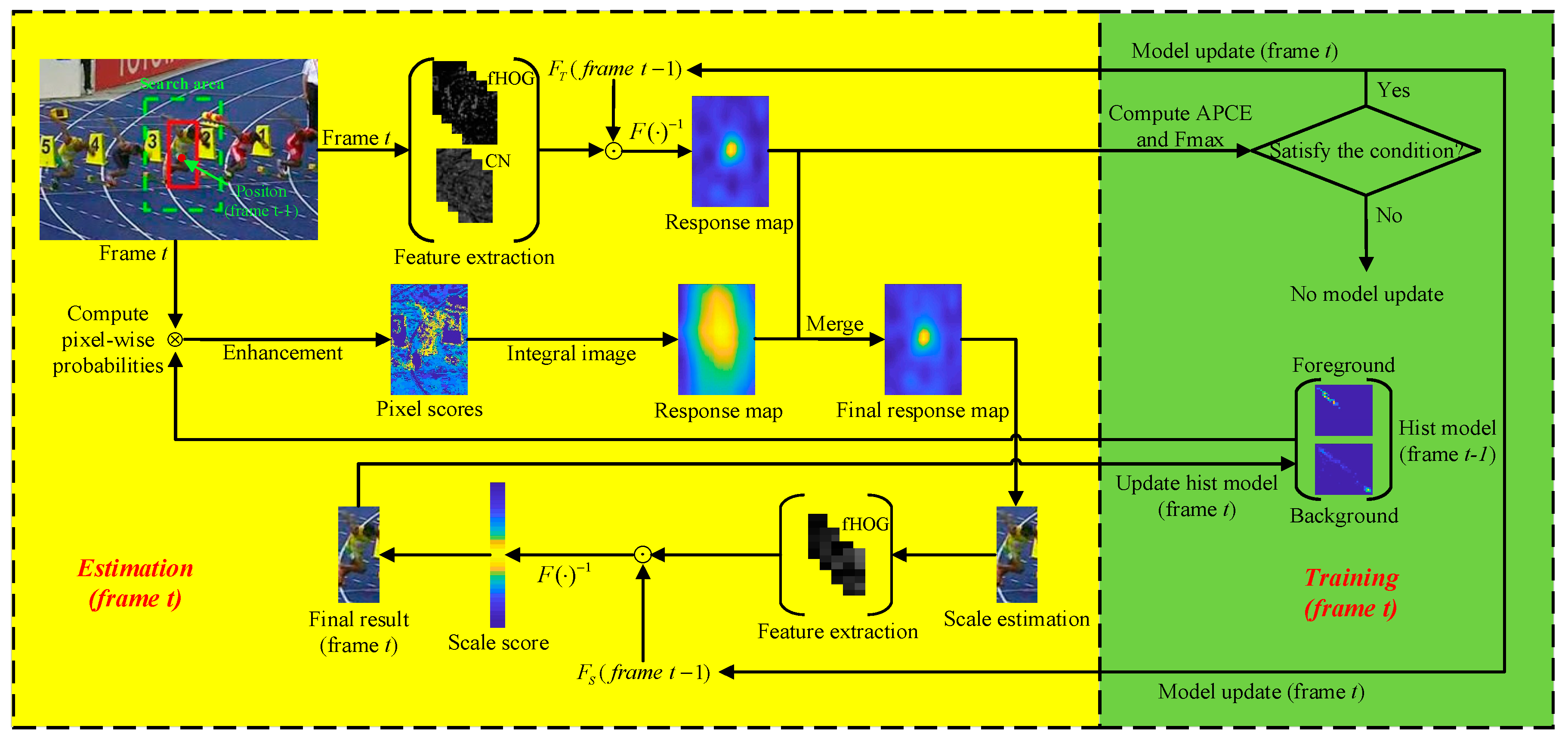
4. Proposed rStaple Tracking Method

In this section, the detailed procedure of the proposed real-time object tracking algorithm termed the robust sum of template and pixel-wise learners (rStaple) is presented. It is based on the Staple [4], an effective tracker which has been widely used in visual tracking.

To initialize the tracker in the first frame of video sequence, the proposed method primarily extracts fHOG [6] and CN [7,8] from the searching area around the given target position. The combination of these two handcrafted features is used to train a translation filter $F_T$. Secondly, the histogram models of the foreground and background are established by current target information. Finally, our tracker trains a 1-D scale filter with fHOG extracted from the initial searching area.

In subsequent frames, firstly, the combination of fHOG and CN of the searching area are extracted to compute a translation filter response map via the translation filter $F_T$ learned in previous frames. Then, we compute the color histogram pixel score map by the histogram model of previous frames, and apply a significant enhancement to the original pixel score map. The final translation score map is a linear combination of the above translation filter response map and the enhanced color histogram score map. Thus, the target position in this frame can be obtained via the final translation score map. Meanwhile, we use fHOG extracted in the current frame and the scale filter learned in the previous frames for scale estimation. Note that the scale estimation can be obtained directly based on the estimated translation result, which greatly reduces the computational cost. Finally, quantitative indicators average peak-to correlation energy (APCE) [44] and $F_{\max }$ are introduced to detect the state of tracking target for the adaptive model update. If the indicators computed from the translation filter response map satisfy the predetermined condition, the translation filter and scale filter are updated in the current frame. Figure 1 illustrates the overall procedure of the proposed rStaple. The area in yellow represents the estimation part in frame $t$ and the green area is the training part in frame $t$. In particular, the training part is performed after estimation.

4.1. Feature Fusion

Researchers have demonstrated that feature extractors usually play the most important role in various object trackers [1]. Therefore, it is necessary to select appropriate features for target modelling. In this paper, fHOG and CN are combined to get a 42-D feature to meet the goal. The combined feature is used to train a translation filter which can learn more information about the tracking target and background.

HOG is one of the most popular features in computer vision. Specifically, it is mainly used to describe the gradient change information in images, and is robust to translation, illumination variation, and posture changes. An input image is divided into many small $2\times 2$ cells when calculating HOG, wherein several adjacent cells are combined into one block. A $[0,\pi )$ region is divided into nine unsigned gradient directions, then each block can be described as a 36-D feature. As an optimization, fHOG [6] divides a $[0,2\pi )$ region into 18 signed gradient directions to obtain a 108-D feature. For reducing the dimensions, the features of four cells in each direction are accumulated to obtain a 27-D feature, while nine unsigned gradient directions of four cells are accumulated to obtain a 4-D feature. Finally, this results in a 31-D feature. In fact, fHOG slightly outperforms HOG via our offline experimental verification. We evaluated the performance of using fHOG instead of HOG on 10 video sequences, under the same experimental conditions. Results show that fHOG operates 22.7% faster than the original HOG with similar accuracy. Therefore, fHOG is adopted in the proposed tracker for both translation estimation and scale estimation.

In some challenging application tasks it is not desirable that trackers simply use fHOG, which lacks robustness to target deformation. Therefore, CN is exploited in the proposed tracking method. CN describes color characteristics of an object and is robust to rotation and deformation. Specifically, it refines the 3-channel RGB features in 11 basic color terms: black, blue, brown, grey, green, orange, pink, purple, red, white, and yellow. In this paper, the mapping given by Weijer et al. [7] is introduced to compute CN, which is learned from the Google image dataset.

4.2. Histogram Significant Enhancement

In conventional tracking tasks, color information of the target generally differs from that of the background, which is a convenient attribute for locating the target more simply. In other words, the target can be found simply via highlighting it in the image. Thus, we can inspect the pixels in the target area with certain rules to significantly enhance the target.

The color histogram tracking builds the color statistical model of the foreground and background. Firstly, the probabilities that each pixel belongs to the foreground and background are calculated separately to obtain the target probability of each pixel. Then, the target probability in a certain area around the pixel is accumulated as the score of the point. Eventually, the difference in color between target and surrounding background is used for tracking.

We can increase the histogram score of the pixels with a higher target probability to highlight the target area in the image. When the target probability $P_t$ of a pixel in Equation (14) is greater than a certain threshold $p_0$, we deploy a significant enhancement to this pixel as:

$$P_t=\{\begin{array}{cc}(P_t-p_0)\cdot r+P_t,\hfill & P_t>p_0\hfill \\ P_t,& else\end{array}$$

(15)

where $r$ denotes a magnification of the enhanced pixel score. By enhancing the high-response pixel, the discrimination of the foreground and background in the searching area can be increased thereby improving the tracking performance. We update the color histogram model in each frame to improve the adaptability of our tracker:

$$\begin{array}{l}{P}_t(O)=(1-{\eta }_{hist})P_{t-1}(O)+{\eta }_{hist}{P}_t{}^{\prime }(O)\\ P_t(B)=(1-{\eta }_{hist})P_{t-1}(B)+{\eta }_{hist}{P}_t{}^{\prime }(B)\end{array}$$

(16)

where ${\eta }_{hist}$ denotes the learning rate of color histogram, $P_{t-1}(O)$ and $P_{t-1}(B)$ denotes foreground model and background model from frame 1 to $t-1$, respectively, and $P_t{}^{\prime }(B)$ and $P_t{}^{\prime }(O)$ denotes model estimated in frame $t$.

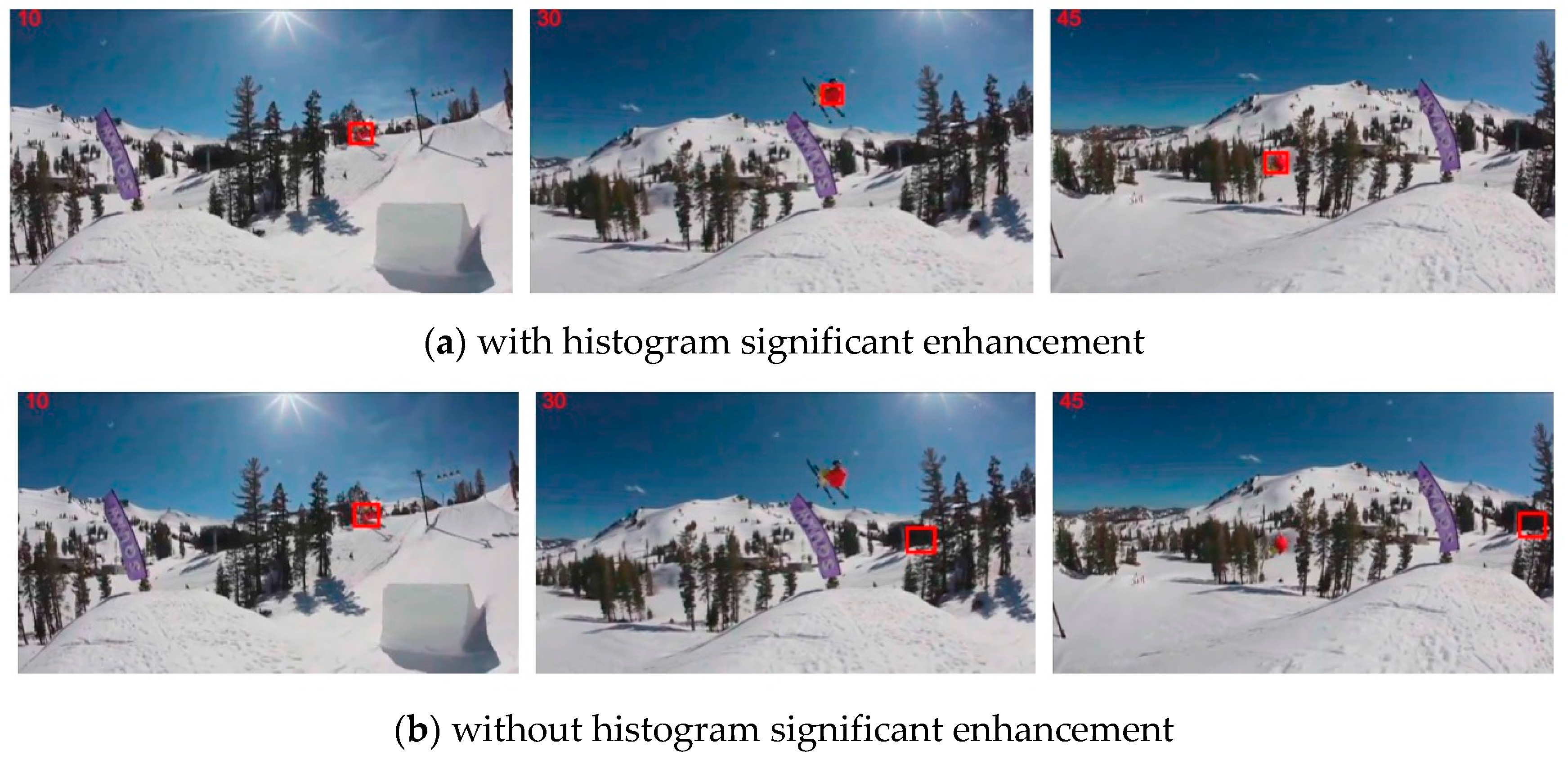
As shown in Figure 2, we test our approach in a video sequence in which the target clearly differs from its background. The tracker with histogram enhancement could keep following the target consistently. In contrast, the tracker without histogram enhancement loses the tracking target in the first few frames since the target is small with a fast motion. This proves that color histogram significant enhancement can weaken the boundary effect of correlation filters to some extent.

Finally, we linearly combine the response map of the translation filter $r_t$ and the color histogram score map $r_{hist}$ to obtain the final translation score map $r$ expressed as:

$$r=\alpha r_{hist}+(1-\alpha )r_t$$

(17)

The position of the maximum in the score map r is the estimated target position in the current frame, and we subsequently perform scale estimation to obtain the final tracking result.

4.3. Scale Estimation

As mentioned above, the target position can be estimated by the combination of translation filter response map and color histogram score map. In addition, a scale pyramid is formulated on the estimated target position to train a scale filter $F_S$. Given the target size $W\times H$ and scale factor $\sigma$, a scale pool $S$ containing $N$ scales can be expressed as:

$$S\in \left\{{\sigma }^n|n=[-\frac{N-1}{2}],[-\frac{N-3}{2}],\dots ,[\frac{N-1}{2}]\right\}$$

(18)

For each scale $s$ in the scale pool $S$, we crop an image patch of size $sW\times sH$ at the center of the estimated target position and interpolate to $W\times H$. fHOG is then extracted and extended into a 1-D vector containing the multi-scale representation of the target. A one-dimensional scale correlation filter can be trained using the features of $N$ scales. The response score of each scale can be calculated by $g(x_s)=\exp (-\frac{{(s-N/2)}^2}{2{\sigma }^2})$, which represents the similarity between the target in the scale $s$ and the learned model. Eventually, the best scale $s^{\prime }$ can be solved from the following optimization problem:

$$s^{\prime }=\underset{s}{\arg \max }\{g(x_s)|s\in S\}$$

(19)

Notice that here only fHOG is adopted to train the scale filter. In order to reduce the errors by inaccurate scale estimation, the result of scale estimation is merely used to update the scale filter, instead of updating both scale filter and translation filter.

4.4. Adaptive Model Update

Most existing correlation filter algorithms update their models at each frame using the estimated tracking result to fit the gradual change of the target appearance. The target position in the next frame is detected by the updated model. However, when the target is occluded or out of view, even for a short time, the accumulation of errors may cause the tracking model to drift. As a result, the model is corrupted and even if the tracking target reappears, the object cannot be redetected by the tracker. MOSSE [18] proposed a peak to sidelobe ratio (PSR) criterion to determine the confidence of the current tracking result. However, this method is not highly effective since a fixed empirical threshold is necessary to guide the selection of updating the model.

In fact, the response map in object tracking can reveal the confidence of tracking to a certain extent. When the peak value is large and fluctuation of the response map is slight, the confidence of the tracking result is considered to be high. If the response map fluctuates intensely and multiple peaks are detected, it indicates that there is background clutter or target occlusion. To solve this problem, two criteria, namely the peak value of the translation filter response map $F_{\max }$ and average peak-to correlation energy (APCE) [44], are adopted to detect the confidence of the tracking result. Specifically, APCE is defined as:

$$APCE=\frac{|F_{\max }-F_{\min }{|}^2}{mean\left({\displaystyle \sum _{w,h}{(F_{w,h}-F_{\min })}^2}\right)}$$

(20)

where $F_{\max }$, $F_{\min }$, and $F_{w,h}$ denote the maximum, minimum, and the value of the coordinate (w, h) in the translation filter response map, respectively. APCE can effectively indicate the confidence of the response map. If the APCE of the response map is large, the peak value is sharp and the fluctuation is slight. Otherwise, the fluctuation is intense and the peak is moderate. In this way, the occlusion or missing state can be determined.

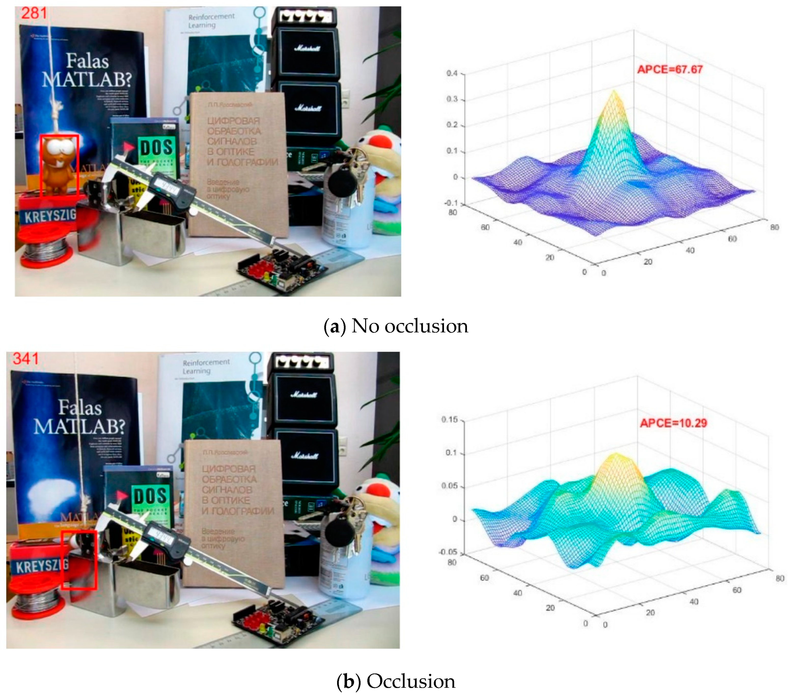
As demonstrated in Figure 3a, the target is not occluded in the ${281}^{th}$ frame. It can be observed that there is only one sharp peak in the response map and the remaining area is relatively flat, wherein the APCE is 67.67. In Figure 3b, the target is severely occluded in the ${341}^{th}$ frame. As a result, there are many local peaks with relatively low values in the response map, among which the highest peak is not obvious and the APCE is 10.29. To summarize, the APCE of the response map can effectively reflect the confidence of the tracking result.

Therefore, in order to improve the tracking robustness, those two criteria are introduced to determine whether to update the model. When the APCE and $F_{\max }$ of the translation filter response map are both greater than their historical average values with certain ratios ${\beta }_1$, ${\beta }_2$, the tracker updates both models of the translation filter $F_T$ and scale filter $F_S$. The filter model corresponds to $\alpha$ in Equation (10), which is used to maximize the response in Equation (12) at the target position. Then the filter model $\alpha$ would be updated as:

$$\begin{array}{l}{\widehat{y}}_t=\{\begin{array}{cc}(1-\eta ){\widehat{y}}_{t-1}+\eta {\widehat{y}}_t,\hfill & APCE\ge {\beta }_1\cdot APC{E}_{avg}\&F_{\max }^t\ge {\beta }_2\cdot F_{\max }^{avg}\hfill \\ {\widehat{y}}_{t-1},& else\end{array}\\ {\widehat{k}}_t^{xx}=\{\begin{array}{cc}(1-\eta ){\widehat{k}}_{t-1}^{xx}+\eta {\widehat{k}}_t^{x{x}^{\prime }},\hfill & APCE\ge {\beta }_1\cdot APC{E}_{avg}\&F_{\max }^t\ge {\beta }_2\cdot F_{\max }^{avg}\hfill \\ {\widehat{k}}_{t-1}^{xx},& else\end{array}\end{array}$$

(21)

where $\eta$ denotes the learning rate of the translation filter and scale filter, ${\widehat{y}}_{t-1}$ and ${\widehat{k}}_{t-1}^{xx}$ denote the parameters estimated from frame 1 to $t-1$, and ${\widehat{y}}_t$ and ${\widehat{k}}_t^{xx}$ denote the parameters estimated from frame $t$ alone.

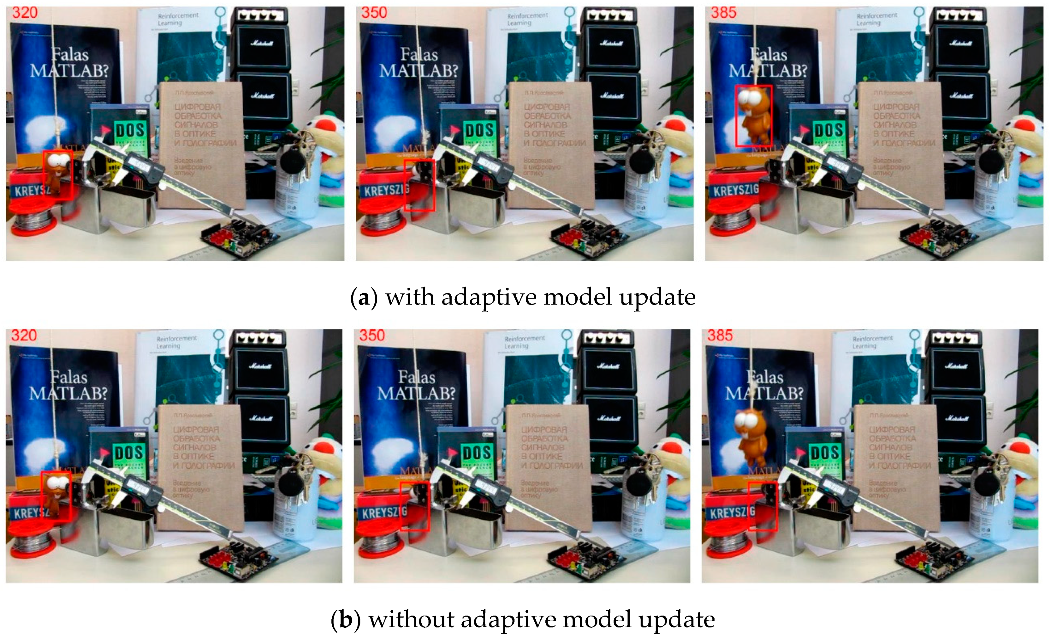
Notice in Figure 4 that the target is partially occluded from the ${320}^{th}$ frame until detaching from occlusion in ${385}^{th}$ frame. Our strategy adaptively determines to hold the current model since the APCE and $F_{\max }$ significantly decrease caused by target occlusion. In this way, the target could be redetected when it appears again. In contrast, if the strategy is not applied, the tracking model would be corrupted during the occlusion and cannot follow the target again when it appears.

4.5. Implementation Details

The proposed rStaple is summarized in Algorithm 1. In this paper, the model of the translation filter is normalized to a fixed size $150\times 150$. The learning rate of translation filter ${\eta }_{cf}$, the learning rate of scale filter ${\eta }_s$, and the learning rate of color histogram ${\eta }_{hist}$ are set to 0.01, 0.025 and 0.04, respectively. The learning rate parameters determine how much target information the tracker can learn in the next frame; too high a learning rate will lead to overlearning of the change of target area and a tendency to drift under the situations of occlusion and being out of view. For scale estimation, the scale factor $\sigma$ is set to 1.02 and the number of scales $N$ in the scale pool is 33. The update thresholds ${\beta }_1$ and ${\beta }_2$ of APCE and $F_{\max }$ in the adaptive model update are 0.57 and 0.38, respectively. The thresholds affect when to perform the model update; if the thresholds are inappropriate, wrong update timing will lead to tracking failure. The parameter $p_0$ is set to 0.71 and $r$ in histogram enhancement is 0.82. If $p_0$ is too high and $r$ is too low, the enhancement will be weak and not beneficial to the performance. Otherwise, the color histogram part will excessively impact the tracker result. We empirically determine these parameters and fix them throughout all the experiments. The parameter of learning rate $\eta$ is determined by Staple and the parameters in scale estimation refer to DSST [21]. Furthermore, we preset the update thresholds and parameters in the histogram enhancement with a few random initial values. After, these values were tested in 10 video sequences which are not included in OTB2013 [10] and OTB2015 [11] to avoid overfitting. Finally, we further fine-tune the values with good performance to obtain the most suitable choice.

Algorithm 1 Outline of our proposed tracking algorithm

Input: Initial bounding box $b_1=(x_1,y_1,w_1,h_1)$, $F_T$, $F_S$

Output: Estimated target bounding box $b_t=(x_t,y_t,w_t,h_t)$

1: repeat

2:  Crop out an image patch z from frame t at the center of $(x_{t-1},y_{t-1})$ and extract its fHOG and CN features;

//Translation estimation

3:  Compute the response map $r_t(z)$ with $F_T$ and $r_{hist}(z)$, estimate target position $(x_t,y_t)$;

//Scale estimation

4:  Construct scale pyramid at estimated target position $(x_t,y_t)$, infer the best scale $s_t$ with $F_S$;

//Adaptive model update

5:  Compute $F_{\max }$ and APCE of $r_t(z)$;

6:  if $F_{\max }$ and APCE satisfy the condition then

7:   Update $F_T$ and $F_S$;

8:  end if

9: until end of video sequence.

5. Experimental Results

We implemented rStaple in the MATLAB 2018b environment on a standard PC with i5-8400 and 16 GB RAM. The proposed tracking algorithm was evaluated on video sequences from OTB2013 [10] and OTB2015 [11] datasets and compared with 12 state-of-the-art trackers, namely, KCF [20], DSST [21], fDSST [22], Staple [4], SRDCF [23], dual linear structured support vector machine (DLSSVM) [45], compressive tracking (CT) [46], CSK [19], long-term correlation tracking (LCT) [24], SiamFC [29], CFNet [30] and ACFN [31]. Of these, SiamFC, CFNet, and ACFN are deep learning-based algorithms. KCF, DSST, fDSST, Staple, SRDCF, LCT, CT, and CSK are correlation filter -based trackers. To show the results clearly and avoid overly dense result curves, the proposed tracker is compared with nine trackers without deep learning on OTB2013. In addition, the deep learning-based algorithms and several trackers that perform well on OTB2013 are compared with our proposed tracker on OTB2015.

5.1. Evaluation Metrics

The OTB2013 and OTB2015 datasets include 11 common challenges in object tracking: illumination variation (IV), scale variation (SV), occlusion (OCC), deformation (DEF), motion blur (MB), fast motion (FM), in-plane rotation (IPR), out-of-plane rotation (OPR), out-of-view (OV), background clutters (BC), and low resolution (LR). Each video sequence also has one or more attributes. The proposed tracker is evaluated by one-pass evaluation (OPE), which initializes the tracker with the ground truth bounding box in the first frame, and subsequent frames are processed by the tracker. We evaluate the performance of the proposed tracker using the following four widely used metrics in Visual Tracking Benchmark dataset:

• Overlap success(OS) rate: the percentage of frames in which the Intersection over Union (IOU) between the estimated target bounding box $b_1$ and the ground truth bounding box $b_0$ is larger than a threshold $t$, i.e., $\frac{b_1\cap b_0}{b_1\cup b_0}>t$.
  Distance precision (DP) rate: the percentage of frames in which the distance between the estimated center location of the target and the ground truth center location is smaller than the threshold.
  Average center location error: the average distance between the estimated center location and the ground truth center location in each frame.
  Average FPS: the average number of frames processed by the trackers in one second.

5.2. Overall Performance

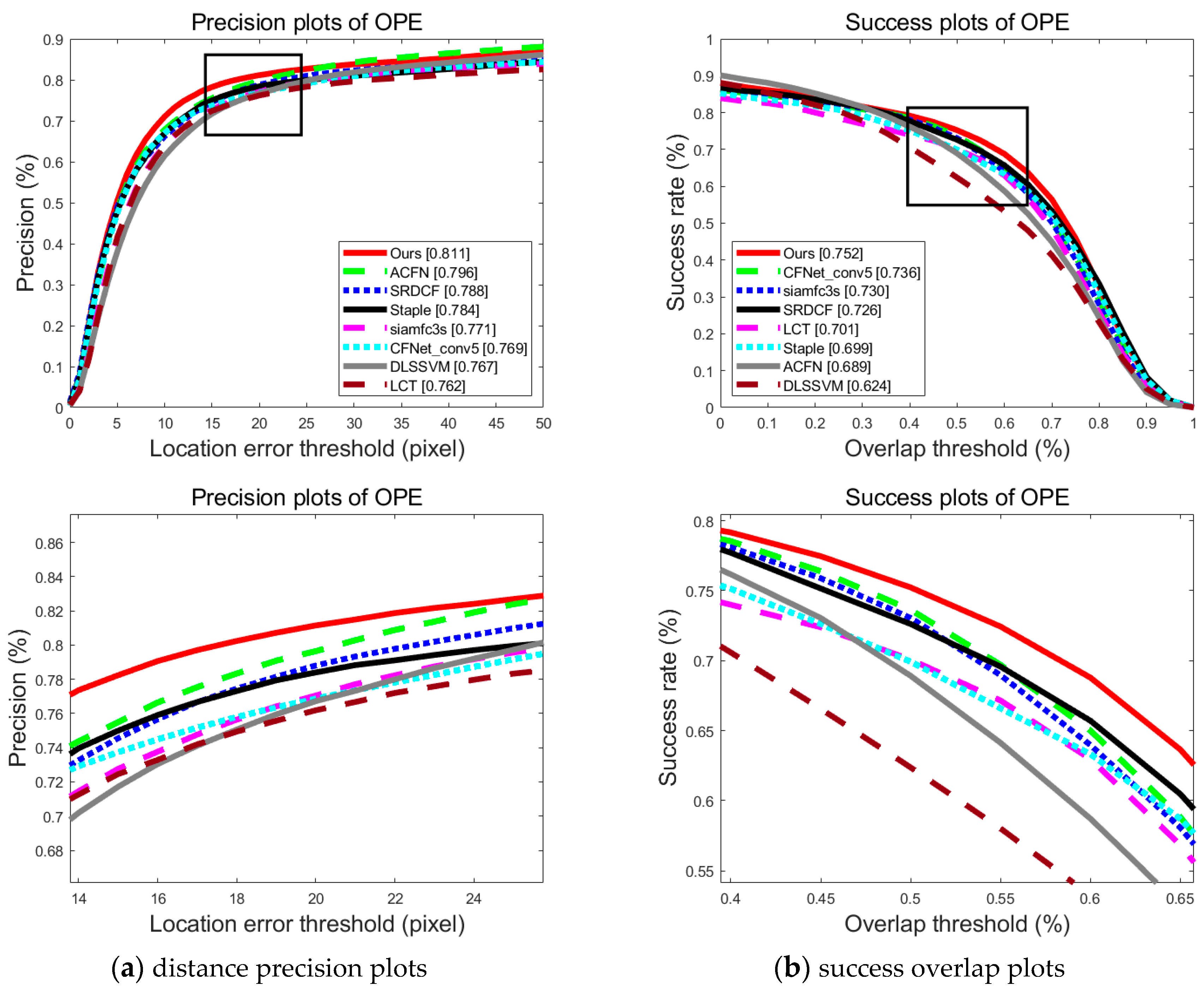
In Figure 5 and Figure 6, we depict the precision rate curve and success rate curve of the proposed algorithm and other compared state-of-the-art algorithms using OPE on OTB2013 and OTB2015 datasets. Figure 5a and Figure 6a show the smooth curve of the distance precision rate when the location error threshold grows from 0 to 50 pixels. Figure 5b and Figure 6b show the curve of the overlap success rate as the overlap threshold increases from 0 to 1. Meanwhile, the data at a predetermined threshold is displayed in the figure. The proposed method exhibits almost the best performance in both evaluation metrics with the increment of the threshold.

Table 1. The performance on OTB2013 dataset of nine trackers.

	Ours	LCT	SRDCF	DLSSVM	Staple	fDSST	DSST	KCF	CSK	CT
DP rate (%)	84.8	84.8	83.8	82.8	78.2	80.3	74	74	54.5	39
OS rate (%)	78.7	81.3	78.1	72.5	73.8	74.7	67	62.3	44.3	26.9
Speed (FPS)	70.3	28.9	8	12.1	86	119	19.4	379	738	152

shows the distance precision rate at a threshold of 20 pixels, overlap success rate at a threshold of 0.5 intersection over union (IOU), and average speed of 10 trackers evaluated on OTB2013. In particular, to accurately evaluate the complexity of these algorithms, the average speed of all trackers was tested on the same hardware environment. The proposed tracker achieves state-of-the-art performance at real-time speed that is superior to many other methods in terms of accuracy. Compared to the baseline Staple, the distance precision rate increases by 6.6%, the overlap success rate increases by 4.9%, and the average center location error increases from 32 to 18.9 pixels according to the results. The overall computational complexity of the proposed algorithm is $O\left(nlogn\right)+O\left(m\right)+O\left(p\right)+O\left(q\right)$. The first part $O(n\log n)$ comes from the correlation filter estimation and $n$ represents the pixels of features which are extracted from the search area. The second part $O(m)$ comes from the color histogram estimation, where $m$ means the search area size. The third part $O(p)$ represents scale estimation, where $p$ is characteristic of the pixels of features in scale pool $S$. The final $O(q)$ is representative of the part of model update. (Normally, $q>p>m$).

Table 2. The performance on OTB2015 dataset of eight trackers.

	Ours	CFNet	ACFN	SiamFC	LCT	Staple	SRDCF	DLSSVM
DP rate (%)	81.1	76.9	79.6	77.1	76.2	78.4	78.8	76.7
OS rate (%)	75.2	73.6	68.9	73	70.1	69.9	72.6	62.4

shows the distance precision rate and overlap success rate of eight trackers evaluated on OTB2015. Since the speed of deep learning-based algorithms depends largely on the hardware facilities such as the GPU, only the accuracy of these trackers is depicted. The proposed method performs better than these state-of-the-art trackers, including deep learning-based algorithms. Moreover, compared to the baseline, the distance precision rate and overlap success rate of our tracker increase by 3.4% and 7.6%, respectively.

Although the difference in distance precision rate and overlap success rate compared to SRDCF and LCT is not obvious in Figure 5, the proposed tracker can achieve better performance at a speed of over two times faster than those methods. Practically, it is desirable for a tracker to provide a better balance between trade-off between efficiency and accuracy.

Distance precision and overlap success rate are shown for 11 different attributes in

Table 3. Distance precision rate (%) of 11 different attributes on OTB2013 dataset.

	Ours	LCT	SRDCF	DLSSVM	Staple	fDSST	DSST	KCF	CSK	CT
FM (17)	73.4	66.5	74.1	74.5	64.2	72.1	51.3	60.2	38.1	23.9
BC (21)	80.5	79.6	80.3	81.4	73	84.2	69.4	75.3	58.5	35.3
MB (12)	70.5	66.4	78.9	75.7	67	78.5	54.4	65	34.2	23.3
DEF (19)	89.9	87.3	85.5	86.9	78.8	74.8	65.8	74	47.6	36.9
IV (25)	84.3	79.2	76.1	75.9	72.7	80.4	73	72.8	48.1	31.8
IPR (31)	81.7	80.2	76.6	81.4	77.3	78.3	76.8	72.5	54.7	36.9
LR (4)	50.8	35.2	51.8	54.6	50.5	47.4	49.7	38.1	41.1	13.1
OCC (29)	88.1	84.5	84.4	82.1	77.5	76.2	70.6	74.9	50	40.1
OPR (39)	85.5	85	81.8	83.7	76.4	77.8	73.6	72.9	54	38.2
OV (6)	79.5	72.8	68	68.8	66.9	68.3	51.1	65	37.9	22.5
SV (28)	82.2	75.8	77.8	76.2	72.1	76.2	73.8	67.9	50.3	40.3

,

Table 4. Overlap success rate (%) of 11 different attributes on OTB2013 dataset.

	Ours	LCT	SRDCF	DLSSVM	Staple	fDSST	DSST	KCF	CSK	CT
FM (17)	70.1	67.6	71.1	69.6	60.5	69.9	50.3	55.7	38	20.3
BC (21)	75.1	76.7	71.5	74.8	69.8	77	62.7	67.2	49.1	28.2
MB (12)	66.6	66.5	76.2	72.7	62.8	73.5	52.8	59.5	33.6	16.2
DEF (19)	85	88.2	80.5	76.7	77.4	72.2	63.1	67.1	37	29.5
IV (25)	74.8	75.4	70.1	65.6	69.2	74.3	68.1	58.1	38.8	24.6
IPR (31)	73.4	77	70.8	69.4	71.4	71.9	67.9	61.5	45.7	21.4
LR (4)	50.6	34.5	52.6	51.2	49.9	45.5	49.7	35.7	39.7	9.8
OCC (29)	82.3	80.5	79	72.4	73.2	69.3	64.6	61.8	40.4	26.5
OPR (39)	77.1	80.3	73.9	71.3	70.6	70.4	64.3	60.8	43.9	23.8
OV (6)	81.5	69.9	70.2	70.7	58.6	67.7	51.2	65	41	23.8
SV (28)	78.7	69.3	78.1	72.5	73.8	74.7	67	62.3	44.3	26.9

,

Table 5. Distance precision rate (%) of 11 different attributes on OTB2015 dataset.

	Ours	CFNet	ACFN	SiamFC	LCT	Staple	SRDCF	DLSSVM
FM (39)	76.6	71.6	74.3	74.3	68.1	71	76.9	73.3
BC (31)	78.1	73.4	75.2	69	73.4	74.9	77.5	74.3
MB (29)	74	63.3	71.2	70.5	66.9	69.9	76.7	75.1
DEF (43)	79.3	69.6	76.8	69.3	68.5	74.7	73	71.3
IV (37)	81.4	70.6	78.4	74.1	74.3	77.8	78.1	74.5
IPR (51)	79.4	76.8	77.4	74.2	78.2	76.8	74.2	79.2
LR (9)	63	76	62.3	84.7	53.7	61	66.3	67.4
OCC (48)	74.3	70.3	74	72.6	67.9	72.4	72.7	72.4
OPR (63)	78.2	74.1	77.7	75.6	74.6	73.8	74	76
OV (14)	75.2	53.6	65.2	66.9	59.2	66.8	60.2	65.8
SV (63)	76.2	72.7	75.3	73.8	67.8	72.4	74.2	71.6

and

Table 6. Overlap success rate (%) of 11 different attributes on OTB2015 dataset.

	Ours	CFNet	ACFN	SiamFC	LCT	Staple	SRDCF	DLSSVM
FM (39)	72.1	68.4	65.7	70.3	65.5	64.5	71.7	63.1
BC (31)	76	69.9	66.3	65.7	70.3	68.8	70.1	64.9
MB (29)	71	62.8	67.6	68.3	65.9	65	72.9	69
DEF (43)	70.9	63.6	62.6	63.7	61.6	65.6	65.9	56.3
IV (37)	76.2	66.7	69.9	71.7	71.5	77.8	73.5	61.1
IPR (51)	69.1	73.2	63.6	69.7	69.4	66.9	65.8	63.5
LR (9)	56.2	73.8	53	77.7	43.6	47.2	62.5	39.2
OCC (48)	72.3	67.4	61.5	68.8	63.1	65.3	67.4	59.2
OPR (63)	70.7	69.1	63.5	70.5	67.6	64.9	66	60.8
OV (14)	71.1	53.6	51.8	62.8	53.1	54.8	55.8	55.6
SV (63)	75.2	73.6	68.9	73	70.1	69.9	72.6	62.4

. The cells in the first row of Table 3, Table 4, Table 5 and Table 6 are abbreviations of attributes in the OTB dataset, and the number of videos that belong to each attribute is in parentheses. The first-ranked tracker is marked in bold and the second-ranked tracker is marked in italics. In Table 3, our tracker ranks first in seven attributes; except for the motion blur attribute, the remaining three attributes are within 4% of the first-ranked tracker. Compared to the baseline Staple, our performance is improved in all attributes, especially in these five attributes: deformation (11.1%), illumination variation (11.6%), occlusion (10.6%), out of view (12.6%), and scale variation (10.1%). In Table 4, our tracker ranks first in three attributes and second in five attributes. Compared to Staple, the performance is improved in all attributes, especially in these four attributes: fast motion (9.6%), deformation (7.6%), occlusion (9.1%), and out of view (22.9%). In Table 5 and Table 6, our tracker ranks first in eight attributes. Compared to the baseline Staple, our performance is improved in all attributes. According to Table 3, Table 4, Table 5 and Table 6, the proposed tracker is extremely apt at handling the occlusion, out of view and scale variation situations. Furthermore, the performance of the proposed tracker in low resolution is relatively poor, which is due to using fHOG because fHOG resizes a $4\times 4$ pixel area to one pixel for calculating the final feature. Most tracking targets with a low resolution attribute are extremely small, and a host of target information is lost after the resize which leads to tracking failure.

The contribution to performance improvement can be generalized to three aspects. Firstly, we apply significant enhancement to the score map of the color histogram. This improves the attention of the tracker to the target and increases the weight of the color histogram with high confidence, thus weakening the boundary effect. Secondly, the combination of fHOG [6] and CN [7,8] strengthens the discriminating ability of the proposed tracker, which facilitates the translation filter locating the target more accurately. Thirdly, we adaptively update the model of the translation filter and scale filter with criteria APCE [44] and $F_{\max }$. When the target is occluded or out of view, the filter model update is terminated. Therefore, this strategy effectively avoids model drift.

5.3. Specific Analysis

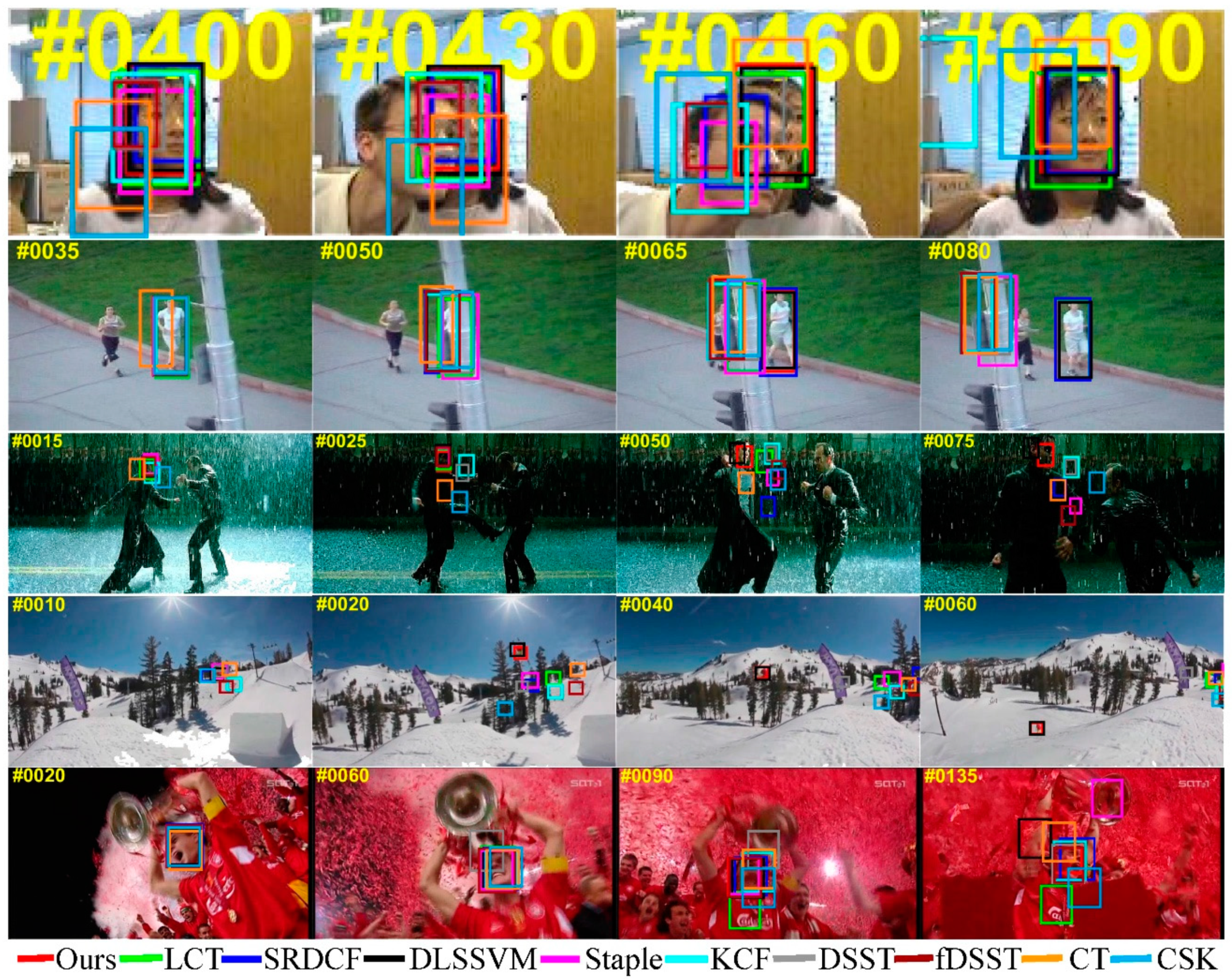
In order to analyze more intuitively, we display the specific tracking results of tested algorithms in five video sequences from OTB2013 and five video sequences from OTB2015. The challenging attributes of these sequences are shown in

Table 7. Attributes of test video sequences on OTB2013.

Sequence	Attributes	Number of Frames
Girl	SV, OCC, IPR, OPR	500
Jogging-2	OCC, DEF, OPR	307
Matrix	IV, SV, OCC, FM, IPR, OPR, BC	100
Skiing	IV, SV, DEF, IPR, OPR	81
Soccer	IV, SV, OCC, MB, FM, IPR, OPR, BC	392

and

Table 8. Attributes of test video sequences on OTB2015.

Sequence	Attributes	Number of Frames
Bolt2	DEF, BC	293
DragonBaby	SV, OCC, MB, FM, IPR, OPR, OV	113
KiteSurf	IV, OCC, IPR, OPR	84
Lemming	IV, SV, OCC, FM, OPR, OV	1336
Panda	SV, OCC, DEF, IPR, OPR, OV, LR	1000

.

Figure 7 shows the tracking results of the proposed algorithm and nine compared trackers on five video sequences from OTB2013. In the first sequence Girl, CT and CSK both lose the target before the ${400}^{th}$ frame. Occlusion occurs between the ${430}^{th}$ frame and ${460}^{th}$ frame. Since the obstruction is similar to the target in color and appearance, Staple, KCF, DSST, and fDSST all drift when the occlusion object leaves. All the tracking bounding boxes follow the occluded object and leave the real target. Our approach successfully avoids model drift when the target is occluded based on the adaptive model update. In the second sequence Jogging-2, the target has a short-term out of view between the ${50}^{th}$ frame and ${65}^{th}$ frame. Only SRDCF, DLSSVM, and rStaple keep tracking when the target reappears at the ${65}^{th}$ frame; the other trackers all fail to track the target again.

The scene of the third sequence, Matrix, is relatively complicated: the target is small and undergoing fast motion and the background changes drastically. From the ${20}^{th}$ frame, CSK, CT, KCF, and DSST fail to track because of the frequent background variance. Staple, LCT and SRDCF lose the target due to fast motion and background clutter. There is also an easily neglected tracking object in the fourth sequence Skiing. The searching area of the correlation filter is related to the size of the estimated bounding box in the current frame, so it is quite difficult to track accurately when the target moves fast and the size of searching area is small. Since DLSSVM abandons correlation filters, only the proposed rStaple and DLSSVM keep tracking till the end. In the last sequence Soccer, DSST fails to track due to fast motion around the $60^{th}$ frame. Both CSK and LCT lose the target in the $90^{th}$ frame due to occlusion and severe background clutter. In the $1{10}^{th}$ frame, the target is completely occluded by the red background and the colors of most areas in the image are very similar, thus, most trackers cannot detect the target precisely. Only rStaple, fDSST, and SRDCF can follow the target when it reappears in the ${135}^{th}$ frame.

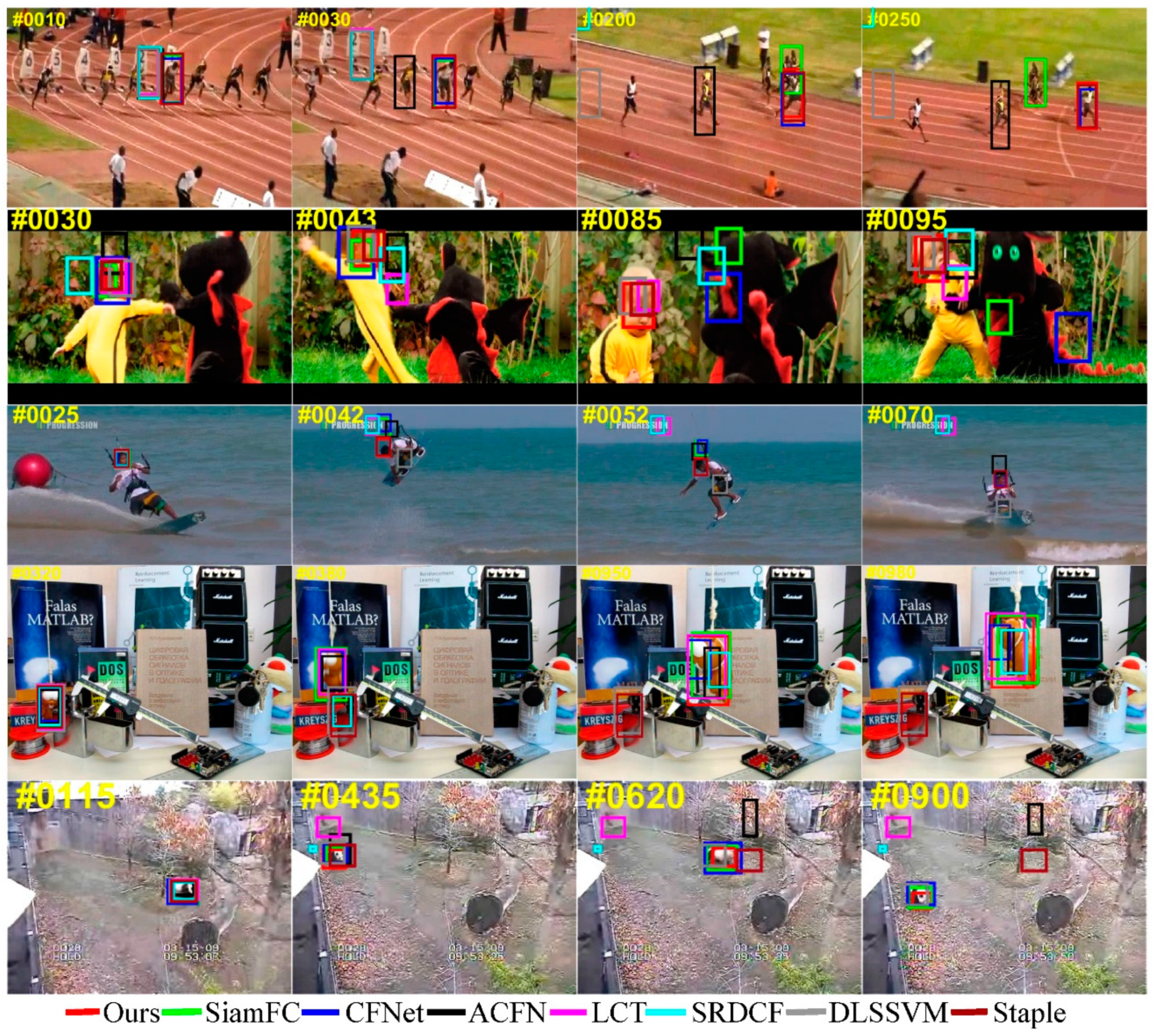
Figure 8 shows the tracking results of the proposed algorithm and seven compared trackers on five video sequences from OTB2015. In the first video sequence Bolt2, ACFN, LCT, SRDCF, and DLSSVM lose the tracking target before the ${10}^{th}$ frame due to fast motion and deformation. In the ${30}^{th}$ frame, ACFN follows a similar object near the target. SiamFC loses the target in the ${200}^{th}$ frame since it is surrounded by several similar objects. In the second sequence DragonBaby, the tracking target is a baby’s head which has a small size and undergoes a fast motion. Many trackers fail to follow the target because of the fast motion. The target in the third sequence, KiteSurf, is also a man’s head. In the ${42}^{th}$ frame, head rotation of the man leads to most trackers losing the target. In the fourth sequence, Lemming, target occlusion occurs between the ${320}^{th}$ frame and ${380}^{th}$ frames. SRDCF, DLSSVM, and Staple fail to track the target due to model drift within this period. ACFN miscalculates the target scale in the ${950}^{th}$ frame and fails to recover. In the last sequence, Panda, LCT and SRDCF lose the target when it turns a corner. In the ${620}^{th}$ frame, Staple and ACFN fail to follow the panda when it passes a tree because of the noisy update of the tracking model.

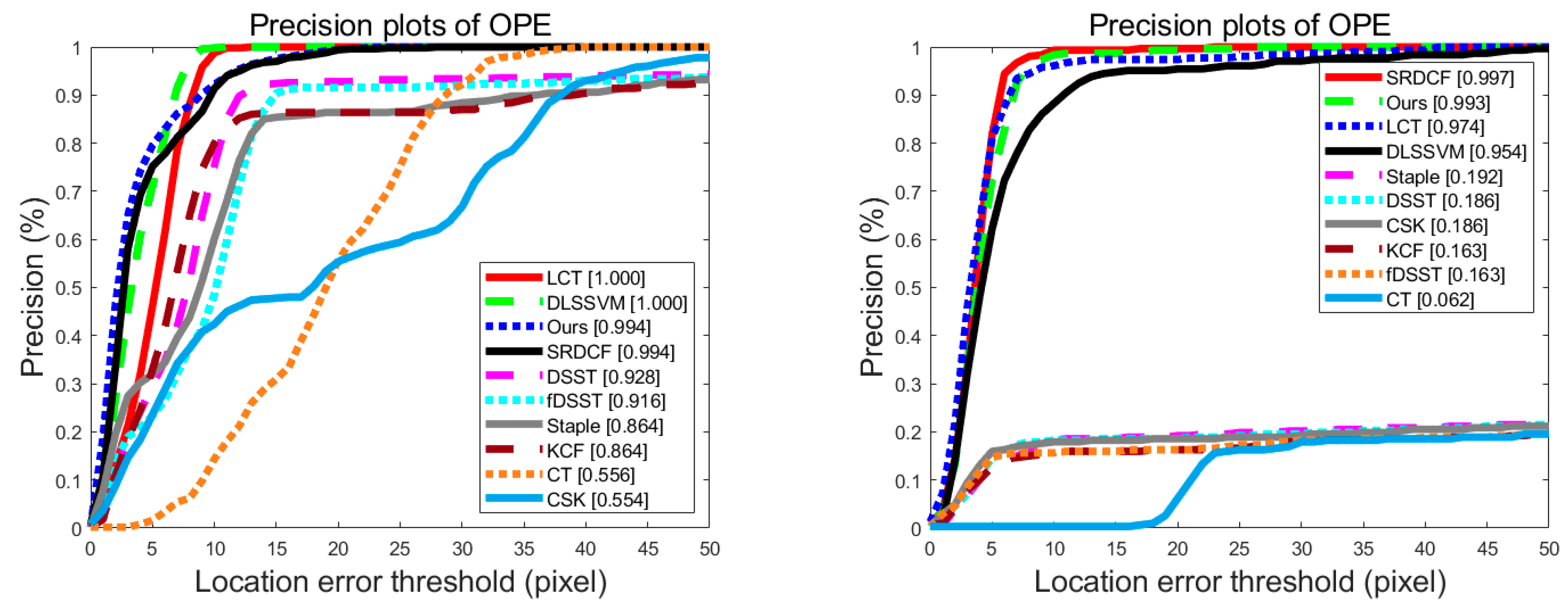
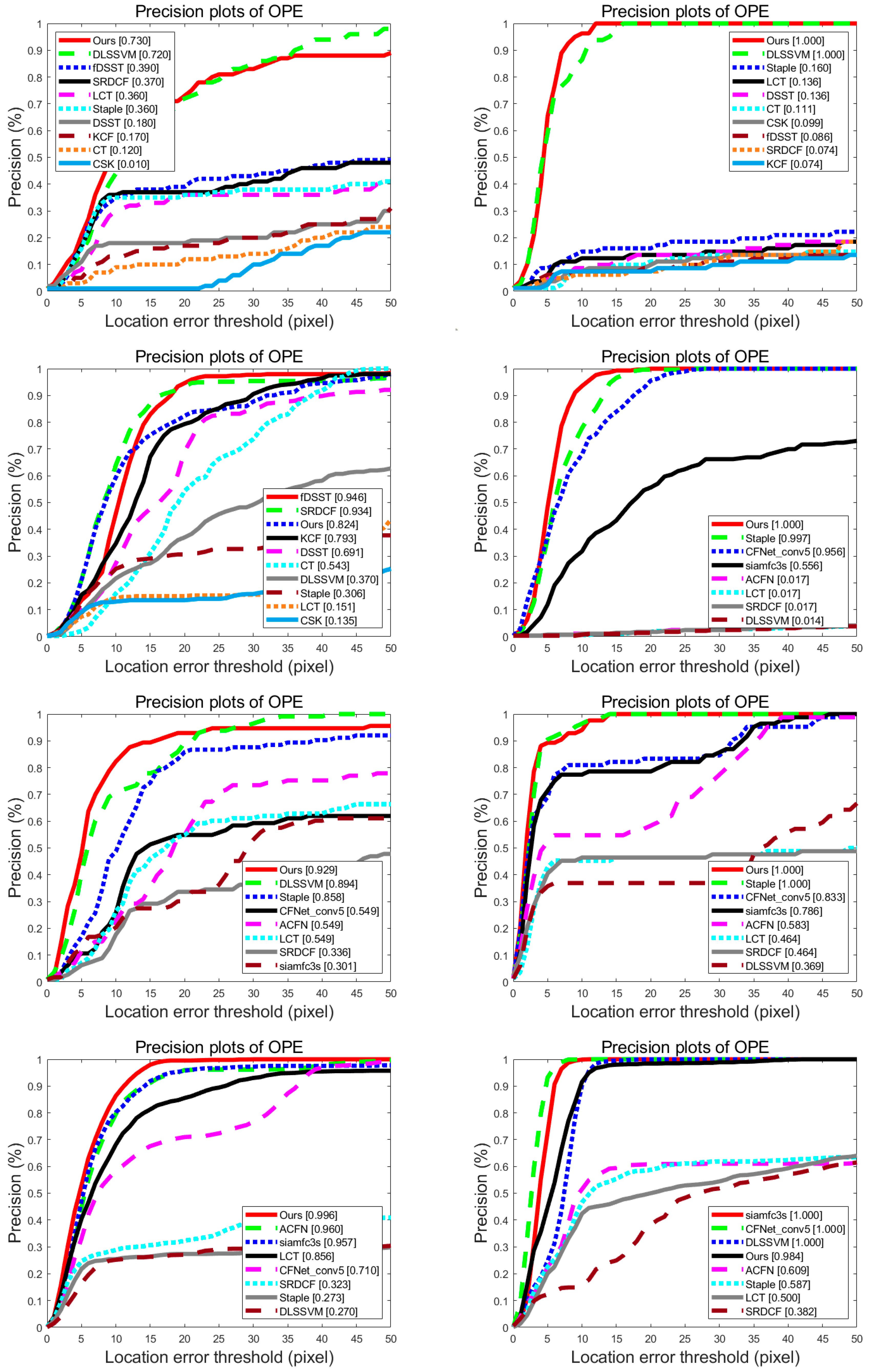
To show the details of the tracking results on ten sequences mentioned above clearly, distance precision rate curves of these sequences are demonstrated in Figure 9. The order from the first figure to the last is: Girl, Jogging-2, Matrix, Skiing, Soccer, Bolt2, DragonBaby, KiteSurf, Lemming, and Panda. As shown in Figure 9, the improvement of the proposed method over the baseline Staple is remarkable. In addition, our method has outstanding performance compared to all of these state-of-the-art trackers.

As illustrated above, the proposed method, rStaple, can handle the challenges of occlusion, fast motion, deformation, and scale variation well in most complex scenes, and achieves state-of-the-art performance.

6. Conclusions

In this paper, we propose a robust object tracking algorithm, rStaple, based on Staple [4]. We first combine fHOG [6] and CN [7,8] to train a translation filter that improves the discriminating ability. Secondly, we use two criteria to adaptively update the model of the translation filter and scale filter, thus alleviating the problem of model drift when the target is occluded or lost. Finally, we apply significant enhancement to the score map of the color histogram, which improves the attention of the tracker to the target. Experimental results show that the proposed tracker achieves state-of-the-art performance at real-time speed. On the other hand, the algorithm still has some defects in several aspects. For example, when encountering objects with intense changes in shape, such as a dancing man or a swimming fish, our tracker tends to lose the target due to the lack of semantic information of the tracking target. For this problem, we will consider extraction of deep features for tracking in subsequent research.