Discontinuity Characterization of Rock Masses through Terrestrial Laser Scanner and Unmanned Aerial Vehicle Techniques Aimed at Slope Stability Assessment


Abstract
1. Introduction
2. Materials and Methods
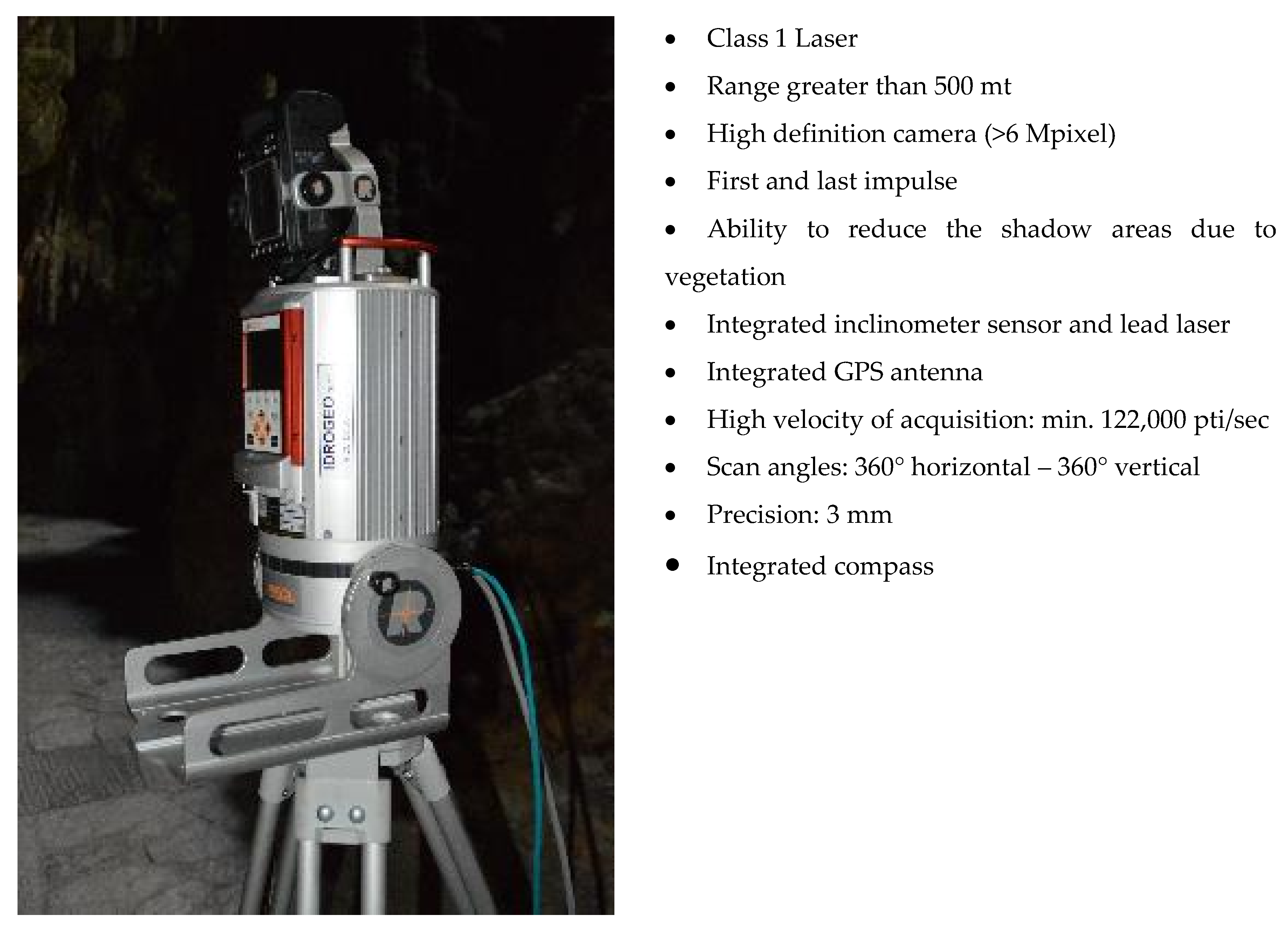
2.1. Survey through Laser Scanner 3D
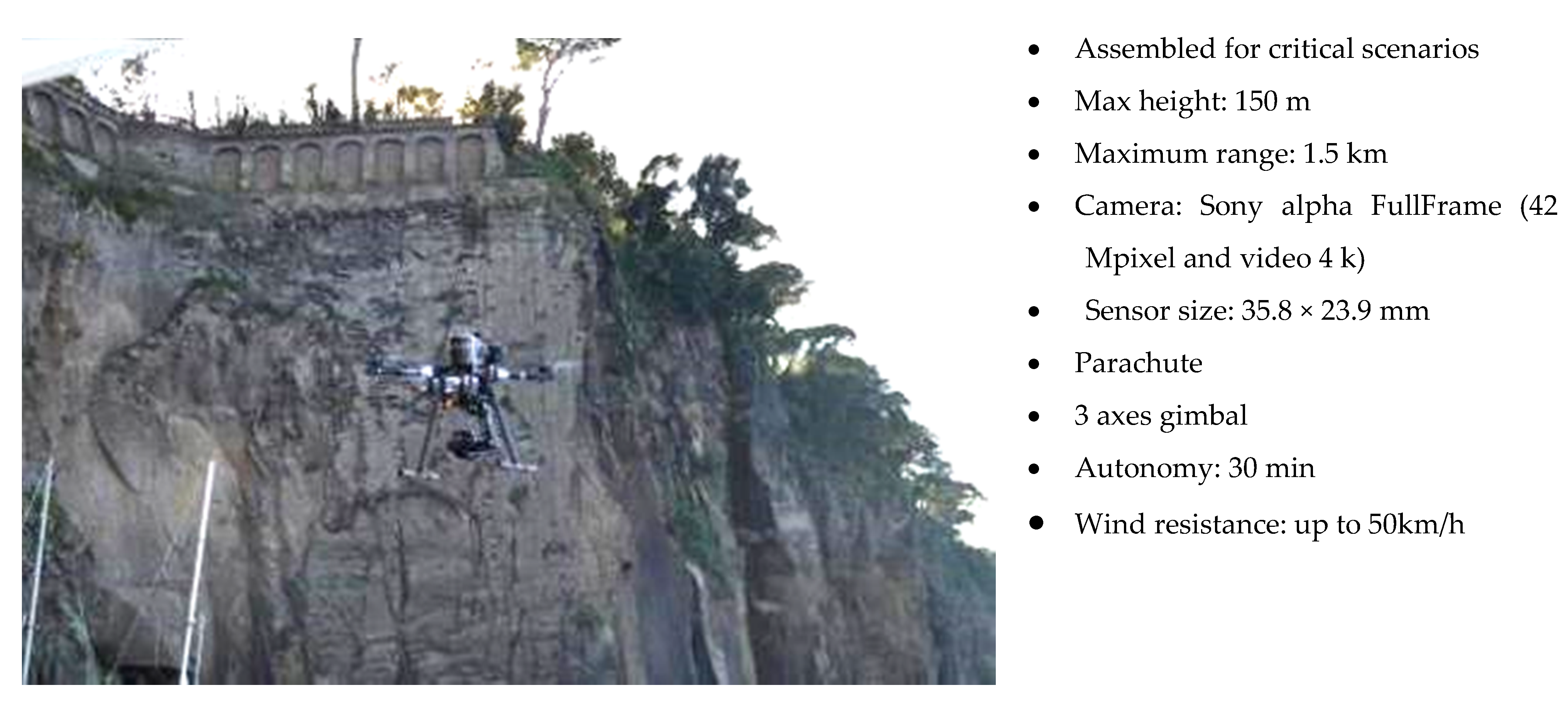
2.2. UAV Photogrammetric Survey
- -
- solve the problems related to lack of stable points where to establish the laser scanner (for instance, at the base of a rock cliff);
- -
- integrate the point cloud from laser scanner in those sectors characterized by no data, due to the relative position between laser and rock cliff;
- -
- survey areas not accessible by land (sea cliffs with no or limited beach, islands, etc.).
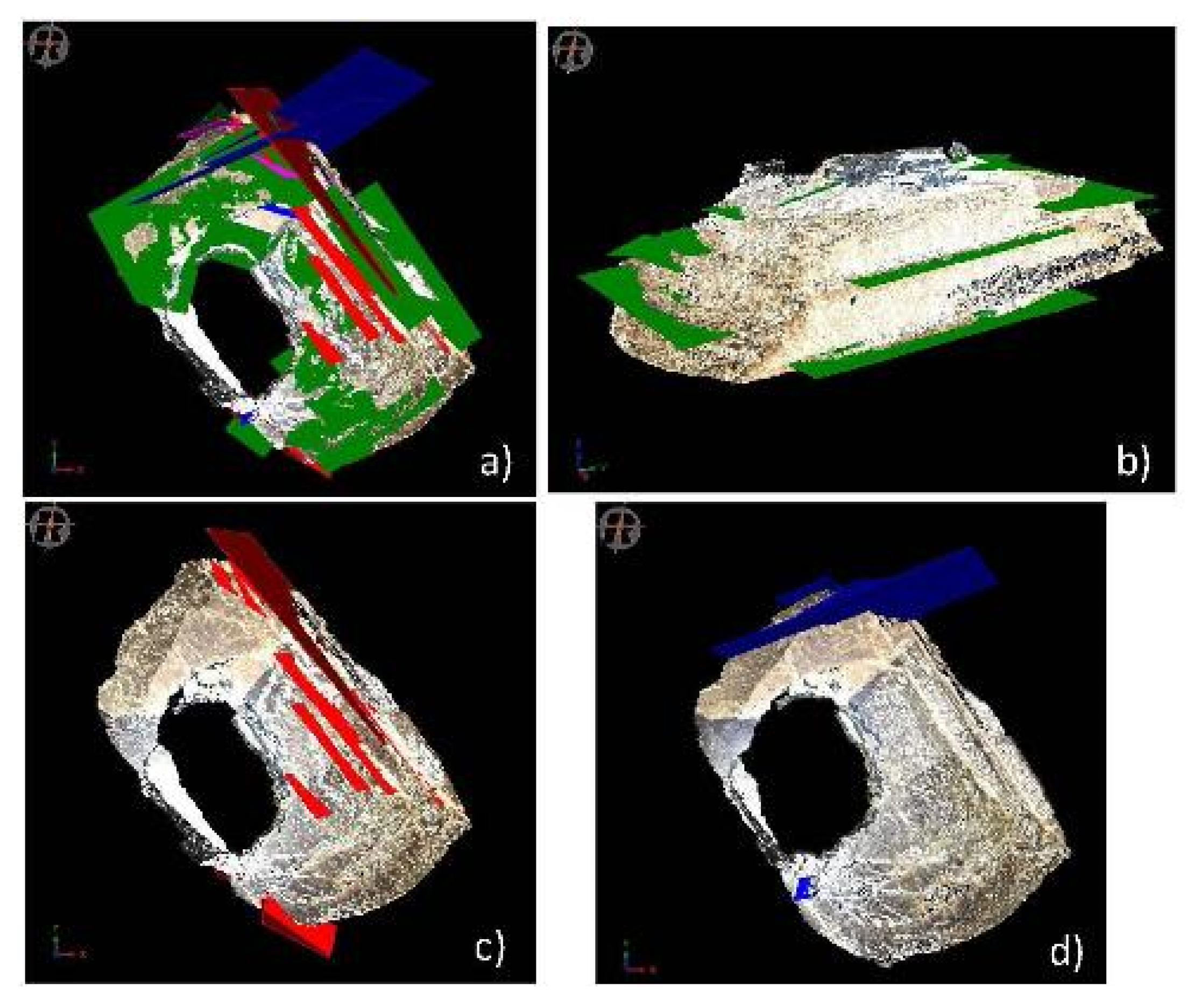
3. Geo-Structural Analysis on Point Clouds
- -
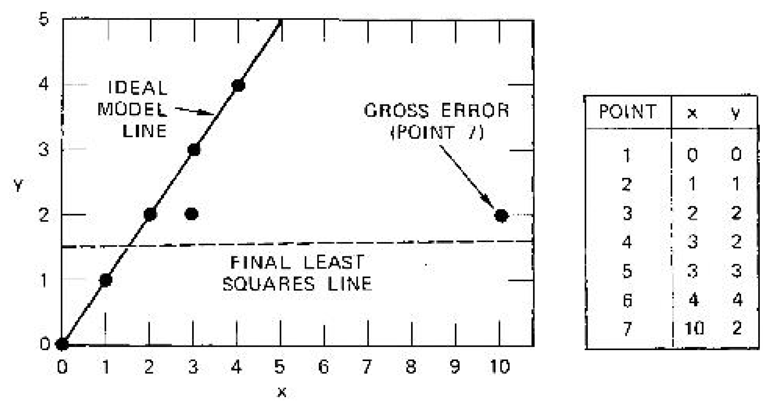
- casual extraction of n = 2 data (minimum necessary to define the model);
- -
- -
- The set containing the highest number of data represents the model:
- -
- the selected model is re-estimated at least squares by using all the points classified as inliers.
- ⮚
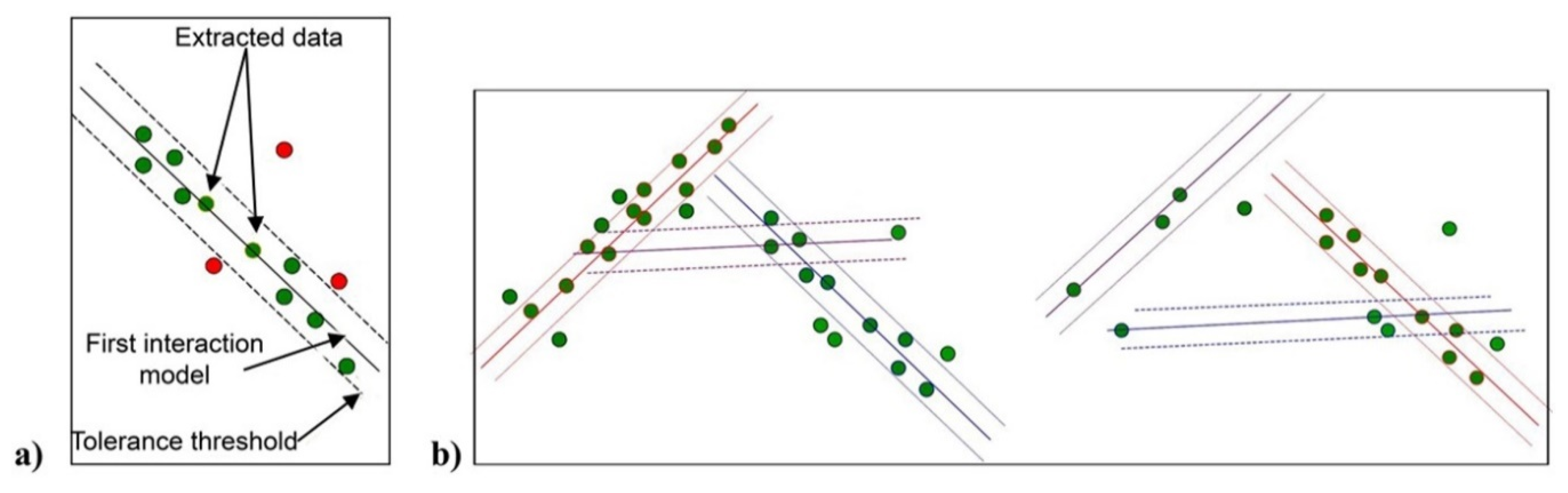
- maximum number of points belonging to the same plane (function of the point density);
- ⮚
- tolerance threshold of the distance between the selected plane and the other points (function of the point cloud accuracy);
- ⮚
- maximum deviation of the vector normal to the selected plane;
- ⮚
- imposition of threshold values, aimed at finalizing the iterative procedure to look for the most suitable planes, without considering those with greater error. This method is semi-automatic, with manual control and validation, since a process of manual selection of the entities to model is at the origin of a mainly computational phase of recognition, computation and conversion of the normals in geo-structural data, dictated by the experience of the operator who keeps a direct control on the dataset of outcomes.
4. Case Studies
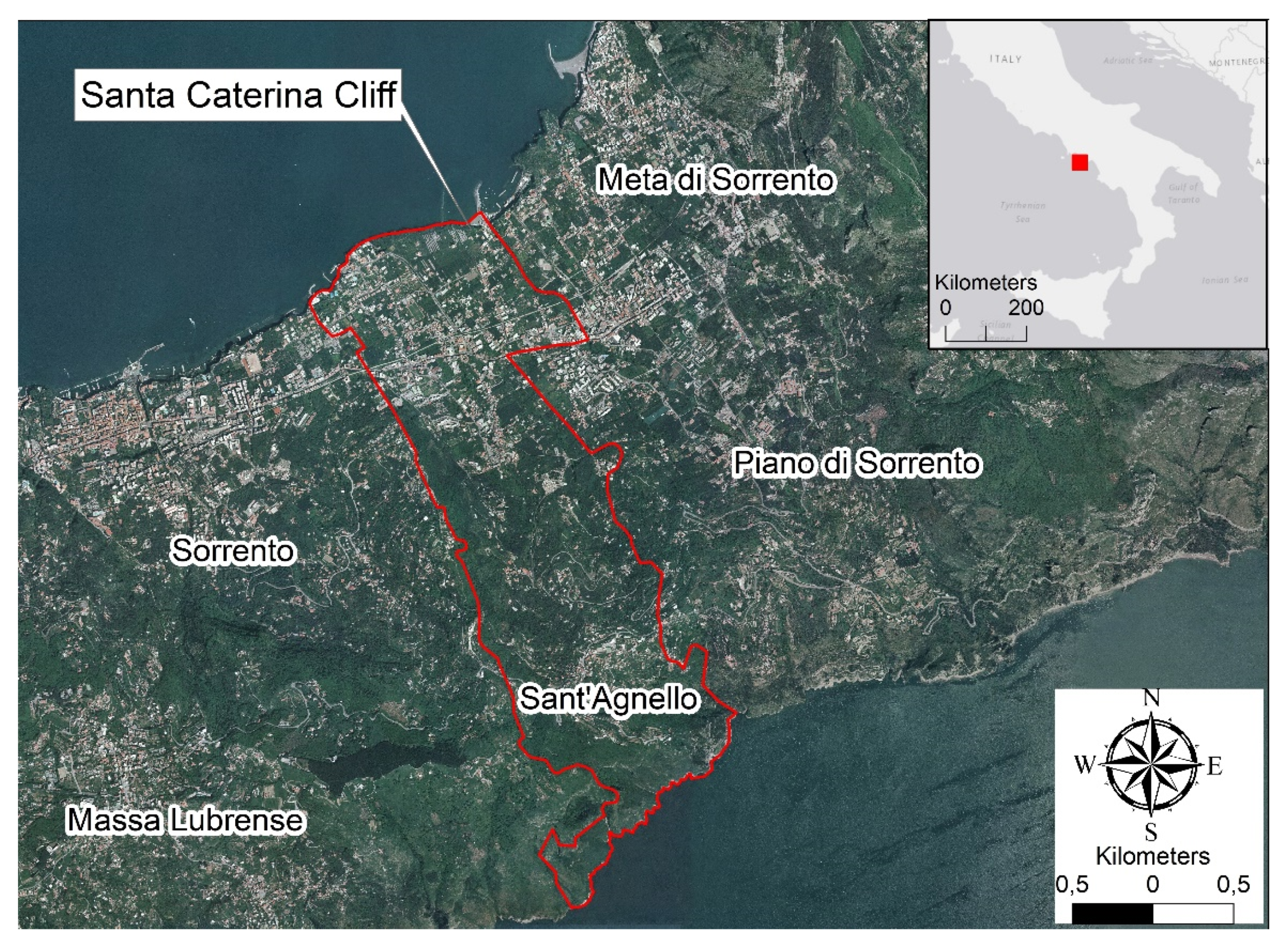
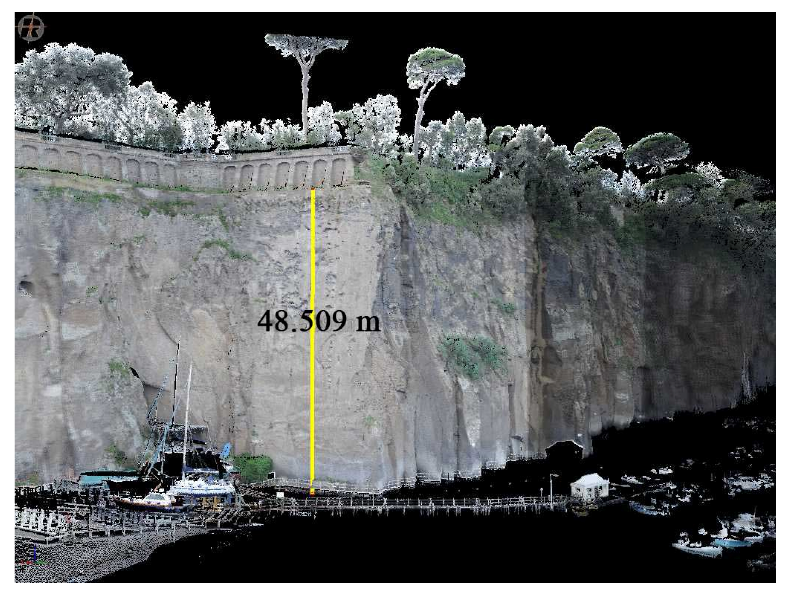
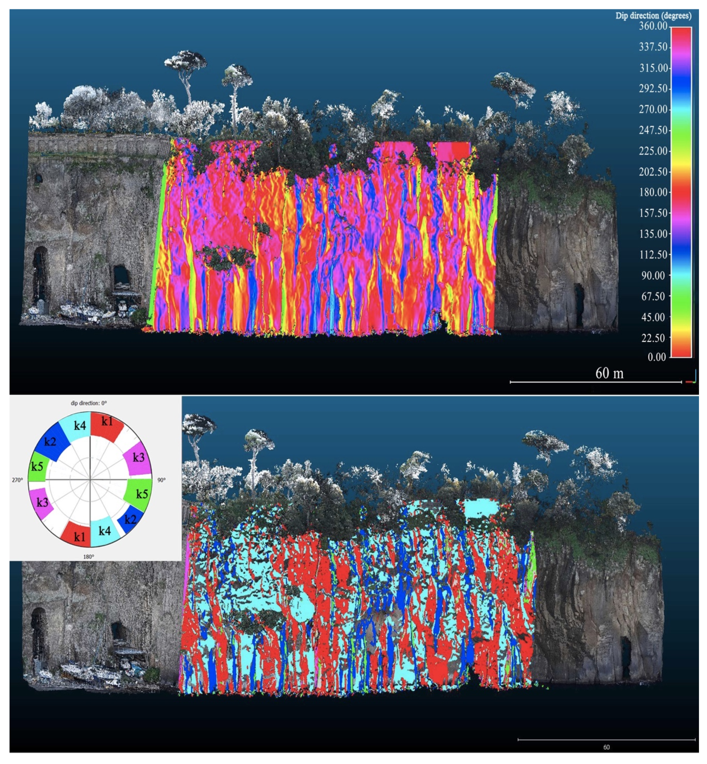
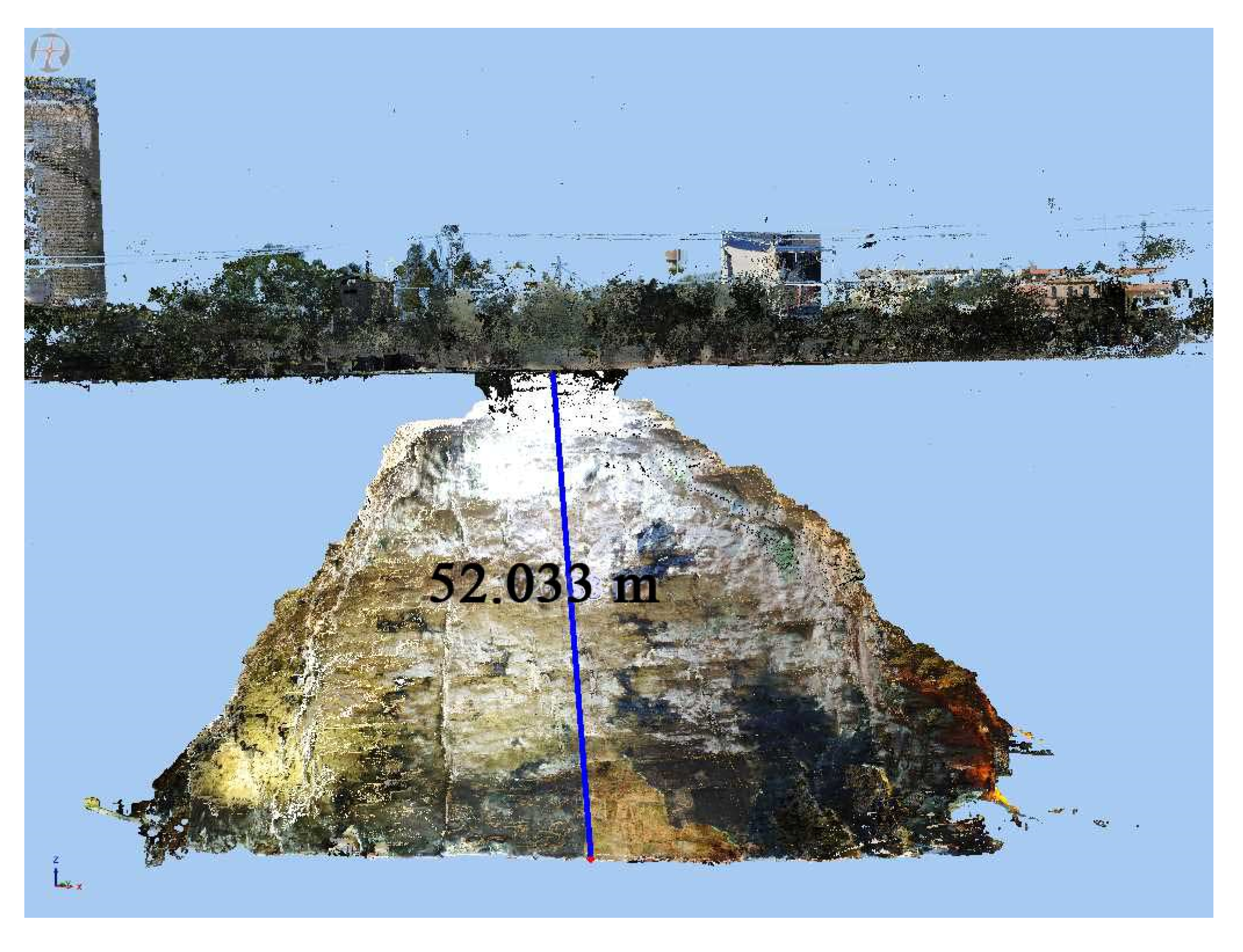
4.1. Santa Caterina
- Sensor size 35.8 × 23.9 mm
- Average distance from the cliff: 40 m
- Ground resolution: 5.6 mm/px
- Overlap H %: 80%
- Overlap L %: 80%
- Photo height (m): 27.31 m
- Photo width (m): 40.91 m
- Photo spacing (m): 5 m
- Interval (m): 16 m
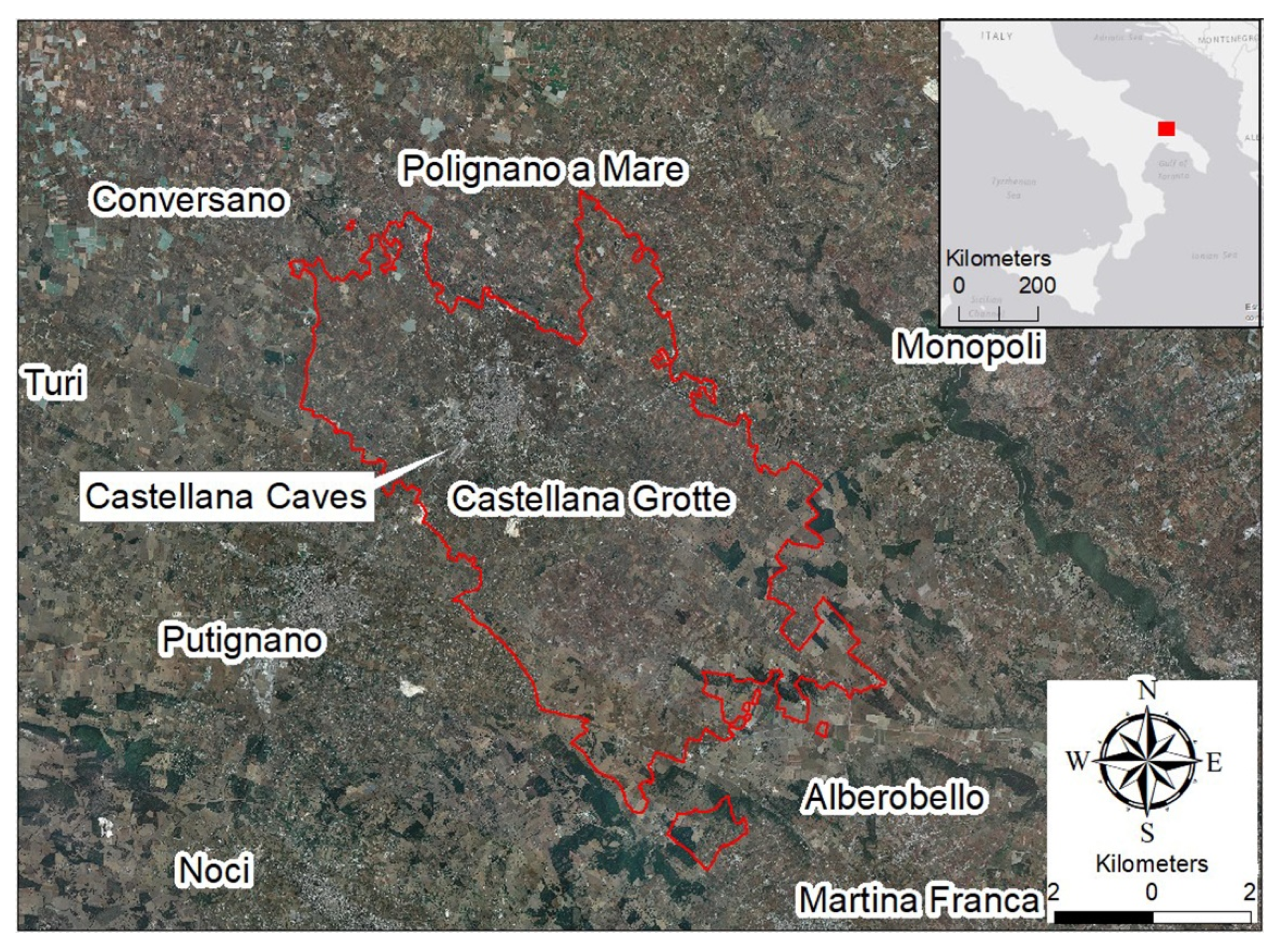
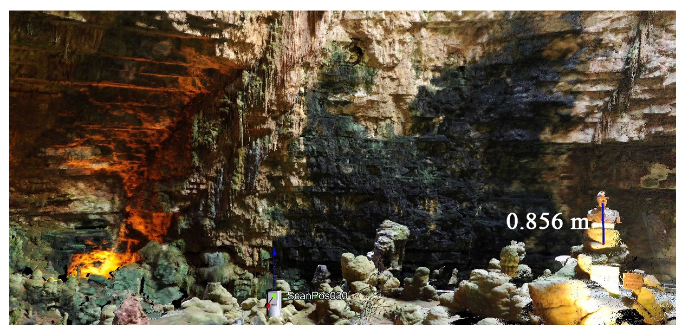
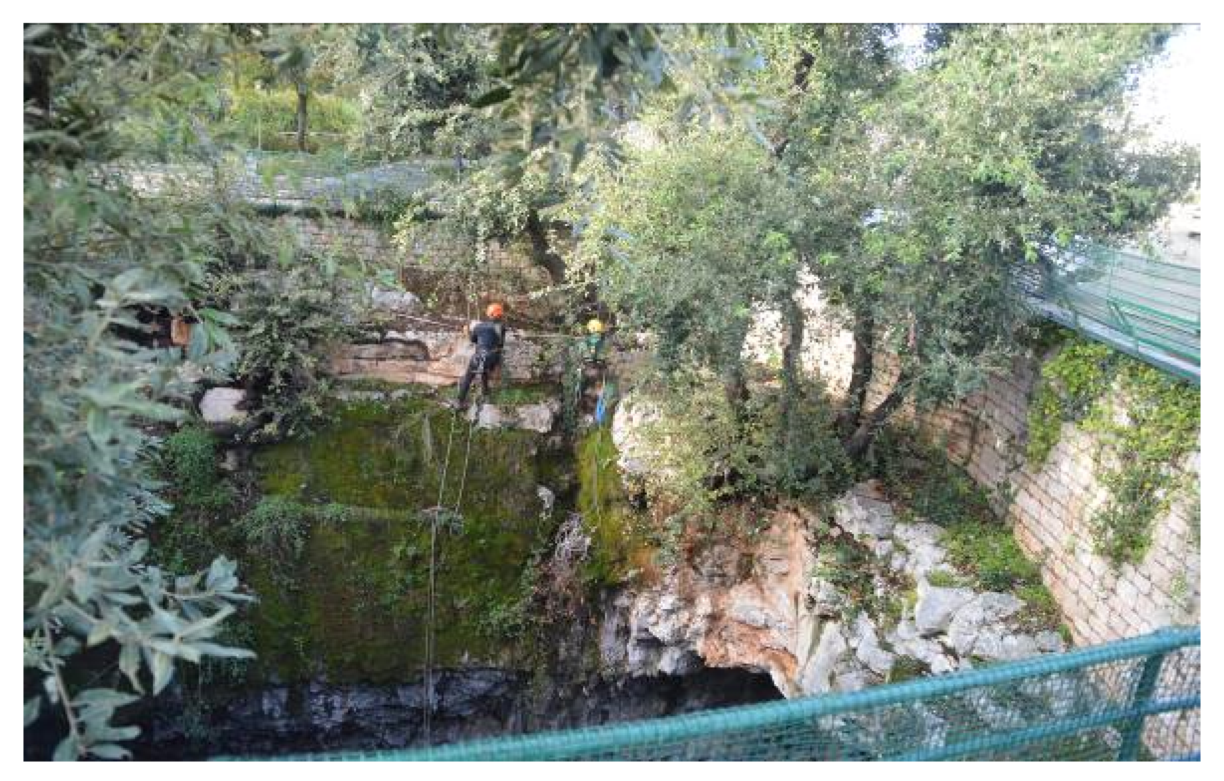
4.2. Castellana Caves
5. Discussion
- ⮚
- Discontinuity analysis by means of remote sensing techniques results in good outcomes through the semi-automatic extraction of data, thus allowing to solve significant logistic problems encountered by the classical survey methods;
- ⮚
- It is possible to perform a geo-structural characterization of the whole area to study, rather than proceeding site per site. This results in a relevant increase in number of data, useful for probabilistic and statistical elaborations;
- ⮚
- The combined procedure allows to provide a large amount of high-resolution data about a variety of parameters that are fundamental for the proper design of stabilization works. Among these, in particular, spacing and persistence of the discontinuities are two main key features in the estimation of the block volume;
- ⮚
- Possibility to highlight the most significant sectors of the investigated areas, where to carry out geomechanical scanlines by geologists/rock climbers, in order to directly acquire parameters such as Joint Compressive Strength, filling materials, etc.;
- ⮚
- The combined use of UAV and TLS is recommended wherever the logistics do not allow to establish TLS scan positions at different locations, and, even more, for frontal views toward the discontinuity planes;
- ⮚
- Increase in the safety of the operators working in the field;
- ⮚
- Less time required for data acquisition (this is a very significant, if not strategic, point in settings as tunnels and quarries);
- ⮚
- Significant reduction in the costs.
Author Contributions
Funding
Conflicts of Interest
References
- Fookes, P.G. Geology for engineers: The geological model, prediction and performance. Q. J. Eng. Geol. 1997, 30, 293–424. [Google Scholar] [CrossRef]
- Miroshnikova, L.S. Engineering-Geologic models as an effective method of schematization of rock masses for purposes of hydrotechnical construction. Hydrotechn. Constr. 1999, 33, 603–612. [Google Scholar] [CrossRef]
- Barla, G.; Barla, M. Continuum and discontinuum modelling in tunnel engineering. Gallerie Grandi Opere Sotter. 2000, 61, 15–35. [Google Scholar]
- Jing, L.; Hudson, J.A. Numerical methods in rock mechanics. Int. J. Rock Min. Sci. 2002, 39, 409–427. [Google Scholar] [CrossRef]
- Jing, L. A review of techniques, advances and outstanding issues in numerical modelling for rock mechanics and rock engineering. Int. J. Rock Min. Sci. 2003, 40, 283–353. [Google Scholar] [CrossRef]
- Garcıa-Jerez, A.; Navarro, M.; Alcali, F.J.; Luzon, F.; Perez-Ruiz, J.A.; Enomoto, T.; Vidal, F.; Ocana, E. Shallow velocity structure using joint inversion of array and h/v spectral ratio of ambient noise: The case of Mula town (SE of Spain). Soil Dyn. Earthq. Eng. 2007, 27, 907–919. [Google Scholar] [CrossRef]
- Stavropoulou, M.; Exadaktylos, G.; Saratsis, G. A combined threedimensional geological—geostatistical—numerical model of underground excavations in rock. Rock Mech. Rock Eng. 2007, 40, 213–243. [Google Scholar] [CrossRef]
- Palma, B.; Ruocco, A.; Lollino, P.; Parise, M. Analysis of the behaviour of a carbonate rock mass due to tunneling in a karst setting. In The Present and Future of Rock Engineering, Proceedings of the 7th Asian Rock Mechanics Symposium, Seoul, Korea, 15–19 October 2012; Han, K.C., Park, C., Kim, J.D., Jeon, S., Song, J.J., Eds.; Korean Society for Rock Mechanics: Seoul, Korea, 2012; pp. 772–781. [Google Scholar]
- Palma, B.; Parise, M.; Reichenbach, P.; Guzzetti, F. Rock-fall hazard assessment along a road in the Sorrento Peninsula, Campania, southern Italy. Nat. Hazards 2012, 61, 187–201. [Google Scholar] [CrossRef]
- Lisjak, A.; Grasselli, G. A review of discrete modeling techniques for fracturing processes in discontinuous rock masses. J. Rock Mech. Geotech. Eng. 2014, 6, 301–314. [Google Scholar] [CrossRef]
- Andriani, G.F.; Parise, M.; Diprizio, G. Uncertainties in the application of rock mass classification and geomechanical models for engineering design in carbonate rocks. In Engineering Geology for Society and Territory, 5. Urban Geology, Sustainable Planning and Landscape Exploitation; Lollino, G., Manconi, A., Guzzetti, F., Culshaw, M., Bobrowsky, P., Luino, F., Eds.; Springer: Berlin, Germany, 2015; Volume 5, pp. 545–548. [Google Scholar]
- Andriani, G.F.; Parise, M. On the applicability of geomechanical models for carbonate rock masses interested by karst processes. Environ. Earth Sci. 2015, 74, 7813–7821. [Google Scholar] [CrossRef]
- Parise, M.; Ravbar, N.; Živanovic, V.; Mikszewski, A.; Kresic, N.; Mádl-Szonyi, J.; Kukuric, N. Hazards in Karst and Managing Water Resources Quality. In Karst Aquifers—Characterization and Engineering; Stevanovic, Z., Ed.; Professional Practice in Earth Sciences; Springer: Berlin, Germany, 2015; pp. 601–687. [Google Scholar]
- Palmer, A.N. Origin and morphology of limestone caves. Geol. Soc. Am. Bull. 1991, 103, 1–21. [Google Scholar] [CrossRef]
- Palmer, A.N. Cave Geology; Cave Books: Dayton, OH, USA, 2007. [Google Scholar]
- Waltham, A.C. The engineering classification of karst with respect to the role and influence of caves. Int. J. Speleol. 2002, 31, 19–35. [Google Scholar] [CrossRef]
- Ford, D.C.; Williams, P. Karst Hydrogeology and Geomorphology; John Wiley and Sons: Chichester, UK, 2007. [Google Scholar]
- Parise, M. Rock failures in karst. In Landslides and Engineered Slopes, Proceedings of the 10th International Symposium on Landslides, Xi’an, China, June 30–4 July 2008; Cheng, Z., Zhang, J., Li, Z., Wu, F., Ho, K., Eds.; Taylor and Francis Group: London, UK, 2008; pp. 275–280. [Google Scholar]
- Andriani, G.F.; Parise, M. Applying rock mass classifications to carbonate rocks for engineering purposes with a new approach using the rock engineering system. J. Rock Mech. Geotechn. Eng. 2017, 9, 364–369. [Google Scholar] [CrossRef]
- Milanovic, P.T. Geological Engineering in Karst; Zebra: Belgrade, Yugoslavia, 2000; p. 347. [Google Scholar]
- Milanovic, P. The environmental impacts of human activities and engineering constructions in karst regions. Episodes 2002, 25, 13–21. [Google Scholar] [CrossRef] [PubMed]
- Stevanovic, Z.; Jemcov, I.; Milanovic, S. Management of karst aquifers in Serbia for water supply. Environ. Geol. 2007, 51, 743–748. [Google Scholar] [CrossRef]
- Parise, M.; Closson, D.; Gutierrez, F.; Stevanovic, Z. Anticipating and managing engineering problems in the complex karst environment. Environ. Earth Sci. 2015, 74, 7823–7835. [Google Scholar] [CrossRef]
- Rosser, N.J.; Petley, D.N.; Lim, M.; Dunning, S.; Allison, R.J. Terrestrial laser scanning for monitoring the process of hard rock coastal cliff erosion. Q. J. Eng. Geol. Hydrogeol. 2005, 38, 363–375. [Google Scholar] [CrossRef]
- Oppikofer, T.; Jaboyedoff, M.; Blikra, L.; Derron, M.H.; Metzger, R. Characterization and monitoring of the Åknes rockslide using terrestrial laser scanning. Nat. Hazards Earth Syst. Sci. 2009, 9, 1003–1019. [Google Scholar] [CrossRef]
- Viero, A.; Teza, G.; Massironi, M.; Jaboyedoff, M.; Galgaro, A. Laser scanning based recognition of rotational movements on a deep-seated gravitational instability: The Cinque Torri case (North-Eastern Italian Alps). Geomorphology 2010, 122, 191–204. [Google Scholar] [CrossRef]
- Riquelme, A.; Tomás, R.; Abellán, A. Characterization of rock slopes through slope mass rating using 3D point clouds. Int. J. Rock Mech. Min. Sci. 2016, 84, 165–176. [Google Scholar] [CrossRef]
- Chen, J.; Zhu, H.; Li, X. Automatic extraction of discontinuity orientation from rock mass surface 3D point cloud. Comput. Geosci. 2016, 95, 18–31. [Google Scholar] [CrossRef]
- Gomes, R.K.; de Oliveira, L.P.L.; Gonzaga, L.; Tognoli, F.M.W.; Veronez, M.R.; de Souza, M.K. An algorithm for automatic detection and orientation estimation of planar structures in LiDAR-scanned outcrops. Comput. Geosci. 2016, 90, 170–178. [Google Scholar] [CrossRef]
- Riquelme, A.; Cano, M.; Tomás, R.; Abellán, A. Identification of Rock Slope Discontinuity Sets from Laser Scanner and Photogrammetric Point Clouds: A Comparative Analysis. Procedia Eng. 2017, 191, 838–845. [Google Scholar] [CrossRef]
- Rengers, N. Terrestrial Photogrammetry: A valuable tool for engineering geological purposes. Rock Mech. Eng. Geol. 1967, 5, 150–154. [Google Scholar]
- Feng, Q.; Sjögren, P.; Stephansson, O.; Jing, L. Measuring fracture orientation at exposed rock faces by using a non-reflector total station. Eng. Geol. 2001, 59, 133–146. [Google Scholar] [CrossRef]
- Slob, S.; Hack, R. 3D terrestrial laser scanning as a new field measurement and monitoring technique. Lect. Notes Earth Sci. 2004, 104, 179–189. [Google Scholar]
- Slob, S.; van Knapen, B.; Hack, R.; Turner, K.; Kemeny, J. Method for automated discontinuity analysis of rock slopes with three-dimensional laser scanning. J. Transp. Res. Board 2005, 1913, 187–194. [Google Scholar] [CrossRef]
- Slob, S.; Hack, H.; Feng, Q.; Röshoff, K.; Turner, A. Fracture Mapping using 3D Laser Scanning Techniques. In Proceedings of the 11th Congress of the International Society for Rock Mechanics, Lisbon, Portugal, 9–13 July 2007; pp. 299–302. [Google Scholar]
- Abellán, A.; Vilaplana, J.M.; Martínez, J. Application of a long-range terrestrial laser scanner to a detailed rockfall study at Vall de Núria (Eastern Pyrenees, Spain). Eng. Geol. 2006, 88, 136–148. [Google Scholar] [CrossRef]
- Sturzenegger, M.; Stead, D. Close-range terrestrial digital photogrammetry and terrestrial laser scanning for discontinuity characterization on rock cuts. Eng. Geol. 2009, 106, 163–182. [Google Scholar] [CrossRef]
- Sturzenegger, M.; Stead, D. Quantifying discontinuity orientation and persistence on high mountain rock slopes and large landslides using terrestrial remote sensing techniques. Nat. Hazards Earth Syst. Sci. 2009, 9, 267–287. [Google Scholar] [CrossRef]
- García-Sellés, D.; Falivene, O.; Arbués, P.; Gratacos, O.; Tavani, S.; Muñoz, J.A. Supervised identification and reconstruction of near-planar geological surfaces from terrestrial laser scanning. Comput. Geosci. 2011, 37, 1584–1594. [Google Scholar] [CrossRef]
- Gigli, G.; Casagli, N. Semi-automatic extraction of rock mass structural data from high resolution LIDAR point clouds. Int. J. Rock Mech. Min. Sci. 2011, 48, 187–198. [Google Scholar] [CrossRef]
- Sturzenegger, M.; Stead, D.; Elmo, D. Terrestrial remote sensing-based estimation of mean trace length, trace intensity and block size/shape. Eng. Geol. 2011, 119, 96–111. [Google Scholar] [CrossRef]
- Jaboyedoff, M.; Oppikofer, T.; Abellán, A.; Derron, M.H.; Loye, A.; Metzger, R.; Pedrazzini, A. Use of LIDAR in landslide investigations: A review. Nat. Hazards 2012, 61, 5–28. [Google Scholar] [CrossRef]
- Brodu, N.; Lague, D. 3D terrestrial lidar data classification of complex natural scenes using a multi-scale dimensionality criterion: Applications in geomorphology. ISPRS J. Photogramm. Remote Sens. 2012, 68, 121–134. [Google Scholar] [CrossRef]
- James, M.R.; Robson, S. Straightforward reconstruction of 3D surfaces and topography with a camera: Accuracy and geoscience application. J. Geophys. Res. Earth Surf. 2012, 117, F03017. [Google Scholar] [CrossRef]
- James, M.R.; Robson, S. Mitigating systematic error in topographic models derived from UAV and ground-based image networks. Earth Surf. Proc. Landf. 2014, 39, 1413–1420. [Google Scholar] [CrossRef]
- Lato, M.J.; Vöge, M. Automated mapping of rock discontinuities in 3D lidar and photogrammetry models. Int. J. Rock Mech. Min. Sci. 2012, 54, 150–158. [Google Scholar] [CrossRef]
- Abellán, A.; Oppikofer, T.; Jaboyedoff, M.; Rosser, N.J.; Lim, M.; Lato, M.J. Terrestrial laser scanning of rock slope instabilities. Earth Surf. Proc. Landf. 2014, 39, 80–97. [Google Scholar] [CrossRef]
- Abellán, A.; Derron, M.H.; Jaboyedoff, M. ‘Use of 3D Point Clouds in Geohazards’ Special Issue: Current Challenges and Future Trends. Remote Sens. 2016, 8, 130. [Google Scholar]
- Riquelme, A.; Abellán, A.; Tomás, R.; Jaboyedoff, M. A new approach for semi-automatic rock mass joints recognition from 3D point clouds. Comput. Geosci. 2014, 68, 38–52. [Google Scholar] [CrossRef]
- Riquelme, A.; Abellán, A.; Tomás, R. Discontinuity spacing analysis in rock masses using 3D point clouds. Eng. Geol. 2015, 195, 185–195. [Google Scholar] [CrossRef]
- Lague, D.; Brodu, N.; Leroux, J.J. Accurate 3D comparison of complex topography with terrestrial laser scanner: Application to the Rangitikei canyon (NZ). ISPRS J. Photogramm. Rem. Sens. 2013, 82, 10–26. [Google Scholar] [CrossRef]
- Fernández, O. Obtaining a best fitting plane through 3D georeferenced data. J. Struct. Geol. 2005, 27, 855–858. [Google Scholar] [CrossRef]
- Jaboyedoff, M.; Metzger, R.; Oppikofer, T.; Couture, R.; Derron, M.; Locat, J.; Turmel, D. New insight techniques to analyze rock-slope relief using DEM and 3D-imaging cloud points: COLTOP-3D software. In Proceedings of the 1st Canada–US Rock Mechanics Symposium, Vancouver, BC, Canada, 27–31 May 2007. [Google Scholar]
- Ester, M.; Kriegel, H.P.; Sander, J.; Xu, X. A density-based algorithm for discovering clusters in large spatial databases with noise. In Proceedings of the Second International Conference on Knowledge Discovery and Data Mining, Portland, OR, USA, 2–4 August 1996; pp. 226–231. [Google Scholar]
- Lato, M.; Diederichs, M.S.; Hutchinson, D.J. Bias correction for view-limited Lidar scanning of rock outcrops for structural characterization. Rock Mech. Rock Eng. 2010, 43, 615–628. [Google Scholar] [CrossRef]
- Khoshelham, K.; Altundag, D.; Ngan-Tillard, D.; Menenti, M. Influence of range measurement noise on roughness characterization of rock surfaces using terrestrial laser scanning. Int. J. Rock Mech. Min. Sci. 2011, 48, 1215–1223. [Google Scholar] [CrossRef]
- Girardeau-Montaut, D. CloudCompare (version 2.8) [GPL Software], OpenSource Project. 2016. Available online: http://www.danielgm.net/cc/ (accessed on 14 November 2019).
- Dewez, T.J.B.; Girardeau-Montaut, D.; Allanic, C.; Rohmer, J.F. A CloudCompare plugin to extract geological planes from unstructured 3D point clouds. ISPRS Int. Arch. Photogramm. Remote Sens. Spat. Inf. Sci. 2016, XLI-B5, 799–804. [Google Scholar] [CrossRef]
- Roncella, R.; Forlani, G.; Remondino, F. Photogrammetry for geological applications: Automatic retrieval of discontinuity orientation in rock slopes. In Proceedings of the International Society for Optics and Photonics, San Diego, CA, USA, 12 May 2004. [Google Scholar]
- Fischler, M.A.; Bolles, R.C. Random sample consensus: A paradigm for model fitting with applications to image analysis and automated cartography. Comm. ACM 1981, 24, 381–395. [Google Scholar] [CrossRef]
- Schnabel, R.; Wahl, R.; Klein, R. Efficient RANSAC for Point-Cloud Shape Detection. Comput. Graph. Forum Citeseer 2007, 26, 214–226. [Google Scholar] [CrossRef]
- Project INTERREG III ALCOTRA; Rockslidetec—Développement d’outils Méthodologiques Pour la Détection et la Propagation des Éboulements de Masse. Final Report. 2002–2006. Available online: http://www.risknat.org/projets/rockslidetec/ (accessed on 14 November 2019).
- Olariu, M.I.; Ferguson, J.F.; Aiken, C.L.; Xu, X. Outcrop fracture characterization using terrestrial laser scanners: Deep-water Jackfork sandstone at Big Rock Quarry, Arkansas. Geosphere 2008, 4, 247–259. [Google Scholar] [CrossRef]
- Vöge, M.; Lato, M.J.; Diederichs, M.S. Automated rockmass discontinuity mapping from 3-dimensional surface data. Eng. Geol. 2013, 164, 155–162. [Google Scholar] [CrossRef]
- Tarsha-Kurdi, F.; Landes, T.; Grussenmeyer, P. Extended RANSAC algorithm for automatic detection of building roof planes from Lidar data. Photogramm. J. Finland 2008, 21, 97–109. [Google Scholar]
- De Vivo, B.; Rolandi, G.; Gans, P.B.; Calvert, A.; Bohrson, W.A.; Spera, F.J.; Belkin, A.E. New constraints on the pyroclastic eruption history of the Campanian volcanic plain (Italy). Mineral. Petrol. 2001, 73, 47–65. [Google Scholar] [CrossRef]
- Pellegrino, A.; Prestininzi, A.; Scarascia Mugnozza, G. Construction of engineering-geology model of crystalline-metamorphic rock masses experiencing deep weathering processes: Example of application to the Allaro and Amusa river basin (Serre Massif, Calabria, Italy). Ital. J. Eng. Geol. Environ. 2008, 1, 33–60. [Google Scholar]
- Calcaterra, D., Parise, M., Eds.; Weathering as a Predisposing Factor to Slope Movements. Geol. Soc. Lond. Eng. Geol. Spec. Publ. 2010, 23, 1–4. [Google Scholar]
- Culshaw, M.G.; Waltham, A.C. Natural and artificial cavities as ground engineering hazards. Q. J. Eng. Geol. 1987, 20, 139–150. [Google Scholar] [CrossRef]
- Parise, M.; Lollino, P. A preliminary analysis of failure mechanisms in karst and man-made underground caves in Southern Italy. Geomorphology 2011, 134, 132–143. [Google Scholar] [CrossRef]
- Del Prete, S.; Parise, M. An overview of the geological and morphological constraints in the excavation of artificial cavities. In Proceedings of the 16th International Congress Speleology, Brno, Czech Republic, 21–28 July 2013; Filippi, M., Bosak, P., Eds.; Czech Speleological Society: Praha, Czech Republic, 2013; Volume 2, pp. 236–241. [Google Scholar]
- Lollino, P.; Martimucci, V.; Parise, M. Geological survey and numerical modeling of the potential failure mechanisms of underground caves. Geosys. Eng. 2013, 16, 100–112. [Google Scholar] [CrossRef]
- Fazio, N.L.; Perrotti, M.; Lollino, P.; Parise, M.; Vattano, M.; Madonia, G.; Di Maggio, C. A three-dimensional back analysis of the collapse of an underground cavity in soft rocks. Eng. Geol. 2017, 238, 301–311. [Google Scholar] [CrossRef]
- Sauro, U. A polygonal karst in Alte Murge (Puglia, Southern Italy). Z. Geomorph. 1991, 35, 207–223. [Google Scholar]
- Parise, M. Surface and subsurface karst geomorphology in the Murge (Apulia, southern Italy). Acta Carsologica 2011, 40, 79–93. [Google Scholar] [CrossRef]
- Gueguen, E.; Formicola, W.; Martimucci, M.; Parise, M.; Ragone, G. Geological controls in the development of palaeo-karst systems of High Murge (Apulia). Rend. Online Soc. Geol. Ital. 2012, 21, 617–619. [Google Scholar]
- Ricchetti, G.; Ciaranfi, N.; Luperto Sinni, E.; Mongelli, F.; Pieri, P. Geodinamica ed evoluzione sedimentaria e tettonica dell’Avampaese Apulo. Mem. Soc. Geol. Ital. 1988, 41, 57–82. [Google Scholar]
- Bosellini, A.; Parente, M. The Apulia Platform margin in the Salento peninsula (southern Italy). Giorn. Geol. 1994, 56, 167–177. [Google Scholar]
- Doglioni, C.; Mongelli, F.; Pieri, P. The Puglia uplift (SE Italy): An anomaly in the foreland of the Apenninic subduction due to buckling of a thick continental lithosphere. Tectonics 1994, 13, 1309–1321. [Google Scholar] [CrossRef]
- Ford, D.C.; Ewers, R.O. The development of limestone cave systems in the dimensions of length and depth. Can. J. Earth Sci. 1978, 15, 1783–1798. [Google Scholar] [CrossRef]
- Palmer, A.N. Patterns of dissolution porosity in carbonate rocks. In Karst Modeling; Palmer, A.N., Palmer, M.V., Sasowsky, I.D., Eds.; Karst Water Institute: Lewisburg, PA, USA, 1999; pp. 71–78. [Google Scholar]
- Sebela, S.; Orndorff, R.C.; Weary, D.J. Geological controls in the development of caves in the south-central Ozarks of Missouri, USA. Acta Carsologica 1999, 28, 273–291. [Google Scholar]
- Harrison, R.W.; Newell, W.L.; Necdet, M. Karstification along an Active Fault Zone in Cyprus; Kuniansky, E.L., Ed.; Water Res Invest Rep, 02-4174; USGS Karst Interest Group: Atlanta, GA, USA, 2002; pp. 45–48. [Google Scholar]
- Klimchouk, A.; Andrejchuk, V. Karst breakdown mechanisms from observations in the gypsum caves of the Western Ukraine: Implications for subsidence hazard assessment. Int. J. Speleol. 2002, 31, 55–88. [Google Scholar] [CrossRef]
- Bruno, E.; Calcaterra, D.; Parise, M. Development and morphometry of sinkholes in coastal plains of Apulia, southern Italy. Preliminary sinkhole susceptibility assessment. Eng. Geol. 2008, 99, 198–209. [Google Scholar] [CrossRef]
- Iovine, G.; Parise, M.; Trocino, A. Breakdown mechanisms in gypsum caves of southern Italy, and the related effects at the surface. Zeit. Geomorph. 2010, 54 (Suppl. 2), 153–178. [Google Scholar] [CrossRef]
- Basso, A.; Bruno, E.; Parise, M.; Pepe, M. Morphometric analysis of sinkholes in a karst coastal area of southern Apulia (Italy). Environ. Earth Sci. 2013, 70, 2545–2559. [Google Scholar] [CrossRef]
- Pepe, M.; Parise, M. Structural control on development of karst landscape in the Salento Peninsula (Apulia, SE Italy). Acta Carsologica 2014, 43, 101–114. [Google Scholar] [CrossRef]
- De Waele, J.; Parise, M. Discussion on the article “Coastal and inland karst morphologies driven by sea level stands: A GIS based method for their evaluation” by Canora F, Fidelibus D, Spilotro, G. Earth Surf. Proc. Landf. 2013, 38, 902–907. [Google Scholar] [CrossRef]
- Anelli, F. First researches of the Italian Institute of Speleology in the Murge of Bari. Le Grotte d’Italia 1938, 2, 11–34. (In Italian) [Google Scholar]
- Anelli, F. Guide to the excursion II. Bari-Alberobello-Selva di Fasano-Castellana Grotte-Bari. In Proceedings of the XVII Italian Congress Geography, Bari-Salerno, Italy, 23–29 April 1957; pp. 69–120. (In Italian). [Google Scholar]
- Parise, M. Some considerations on show cave management issues in Southern Italy. In Karst Management; Van Beynen, P.E., Ed.; Springer: Berlin, Germany, 2011; pp. 159–167. [Google Scholar]
- Parise, M.; Proietto, G.; Savino, G.; Tartarelli, M. Ripresa delle attività esplorative alle Grotte di Castellana: Primi risultati e prospettive future. Grotte e Dintorni 2002, 4, 179–186. [Google Scholar]
- Lollino, P.; Parise, M.; Reina, A. Numerical analysis of the behavior of a karst cave at Castellana-Grotte, Italy. In Proceedings of the 1st International UDEC Symposium “Numerical Modeling of Discrete Materials”, Bochum, Germany, 29 September–1 October 2004; Konietzky, H., Ed.; Taylor and Francis Group: London, UK, 2004; pp. 49–55. [Google Scholar]
- Zupan Hajna, N. Incomplete Solution: Weathering of Cave Walls and the Production, Transport and Deposition of Carbonate Fines. Carsologica, ZRC, Postojna-Ljubljana; Založba ZRC: Ljubljana, Slovenija, 2003. [Google Scholar]
- Davis, G.D.; Mosch, C. Pebble indentations: A new speleogen from a Colorado Cave. Bull. Natl. Speleol. Soc. 1988, 50, 17–20. [Google Scholar]
- Fookes, P.G.; Hawkins, A.B. Limestone weathering: Its engineering significance and a proposed classification scheme. Quart. J. Eng. Geol. 1988, 21, 7–31. [Google Scholar] [CrossRef]
- Waltham, A.C.; Fookes, P.G. Engineering classification of karst ground conditions. Q. J. Eng. Geol. Hydrogeol. 2003, 3, 101–118. [Google Scholar] [CrossRef]
- Parise, M.; Trisciuzzi, M.A. Geomechanical characterization of carbonate rock masses in underground karst systems: A case study from Castellana-Grotte (Italy). In Karst and Cryokarst; Tyc, A., Stefaniak, K., Eds.; Studies of the Faculty of EarthSciences, University of Silesia: Sosnowiec-Wroclaw, Poland, 2007; Volume 45, pp. 227–236. [Google Scholar]
- Waltham, T.; Bell, F.; Culshaw, M. Sinkholes and Subsidence; Springer: Chichester, UK, 2005. [Google Scholar]
- Parise, M.; Gunn, J. (Eds.) Natural and Anthropogenic Hazards in Karst Areas: Recognition, Analysis and Mitigation; special publication 279; Geological Society: London, UK, 2007. [Google Scholar]
- Parise, M. Sinkholes. In Encyclopedia of Caves, 3rd ed.; White, W.B., Culver, D.C., Pipan, T., Eds.; Academic Press, Elsevier: London, UK, 2019; pp. 934–942. [Google Scholar]
- Gutierrez, F.; Parise, M.; De Waele, J.; Jourde, H. A review on natural and human-induced geohazards and impacts in karst. Earth-Sci. Rev. 2014, 138, 61–88. [Google Scholar] [CrossRef]
- Parise, M.; Federico, A.; Delle Rose, M.; Sammarco, M. Karst terminology in Apulia (southern Italy). Acta Carsologica 2003, 32, 65–82. [Google Scholar] [CrossRef]
- Castiglioni, B.; Sauro, U. Large collapse dolines in Puglia (southern Italy): The cases of “Dolina Pozzatina” in the Gargano Plateau and of “Puli” in the Murge. Acta Carsologica 2000, 29, 83–93. [Google Scholar] [CrossRef]
- Delle Rose, M.; Federico, A.; Parise, M. Sinkhole genesis and evolution in Apulia, and their interrelations with the anthropogenic environment. Nat. Hazards Earth Syst. Sci. 2004, 4, 747–755. [Google Scholar] [CrossRef]
- Simone, O.; Fiore, A. Five large collapse dolines in Apulia (Southern Italy)—The Dolina Pozzatina and the Murgian Puli. Geoheritage 2014, 6, 291–303. [Google Scholar] [CrossRef]
- ISRM. Suggested methods for the quantitative description of discontinuities in rock masses. Int. J. Rock Mech. Min. Sci. Geomech. Abs. 1978, 15, 319–368. [Google Scholar]
- Barton, N.; Lien, R.; Lunde, J. Engineering classification of rock masses for design of tunnel support. Rock Mech. 1974, 6, 189–236. [Google Scholar] [CrossRef]
- Barton, N.; Lien, R.; Lunde, J. Estimation of support requirement for underground excavation. In Proceedings of the 16th US Symposium Rock Mechanics, Minneapolis, MN, USA, 22–24 September 1975; University of Minnesota: Minneapolis, MN, USA, 1975; pp. 163–178. [Google Scholar]
- Bieniawski, Z.T. Geomechanics classification of rock masses and its application in tunnelling. In Proceedings of the 3rd International Congress Rock Mechanics, Denver, CO, USA, 1–7 September 1974; Volume 2A, pp. 27–32. [Google Scholar]
- Bieniawski, Z.T. Engineering Rock Mass Classifications; John Wiley and Sons: Chichester, UK, 1989. [Google Scholar]
- Romana, M. New adjustment ratings for application of Bieniawski classification to slopes. In Proceedings of the International Symposium Role Rock Mechanics, Zacatecas, Mexico, 2–4 September 1985; pp. 49–53. [Google Scholar]
- Hoek, E.; Brown, E.T. Practical estimates of rock mass strength. Int. J. Rock Mech. Mining Sci. Geomech. Abs. 1997, 34, 1165–1186. [Google Scholar] [CrossRef]
- Hoek, E.; Marinos, P.; Benissi, M. Applicability of the geological strength index (GSI) classification for very weak and sheared rock masses. The case of the Athens Schist Formation. Bull. Eng. Geol. Environ. 1998, 57, 151–160. [Google Scholar] [CrossRef]
- Marinos, P.; Hoek, E. Estimating the geotechnical properties of heterogeneous rock masses such as flysch. Bull. Eng. Geol. Environ. 2001, 60, 85–92. [Google Scholar] [CrossRef]
- Tomás, R.; Delgado, J.; Serón Ganez, J.B. Modification of slope mass rating (SMR) by continuous functions. Int. J. Rock Mech. Min. Sci. 2007, 44, 1062–1069. [Google Scholar] [CrossRef]
- Ferrero, A.M.; Forlani, G.; Roncella, R.; Voyat, H.I. Advanced geostructural survey methods applied to rock mass characterization. Rock Mech. Rock Eng. 2009, 42, 631–665. [Google Scholar] [CrossRef]
- Lato, M.; Kemeny, J.; Harrap, R.M.; Bevan, G. Rock bench: Establishing a common repository and standards for assessing rockmass characteristics using LiDAR and photogrammetry. Comput. Geosci. 2013, 50, 106–114. [Google Scholar] [CrossRef]


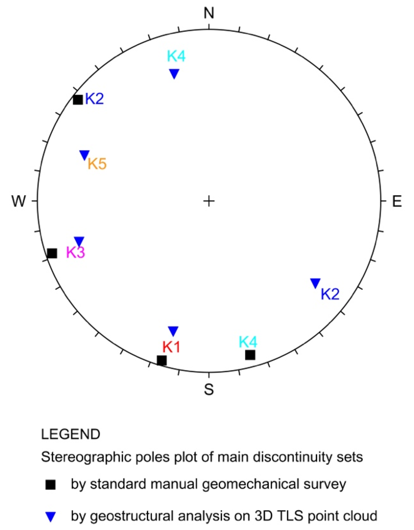
| Set | Dip Direction | Dip |
|---|---|---|
| K1 | 15 | 77 |
| K2 | 308 | 76 |
| K3 | 72 | 77 |
| K4 | 165 | 75 |
| K5 | 110 | 75 |
| Set | Dip Direction | Dip |
|---|---|---|
| K1 | 17 | 89 |
| K2 | 128 | 88 |
| K3 | 72 | 88 |
| K4 | 345 | 86 |
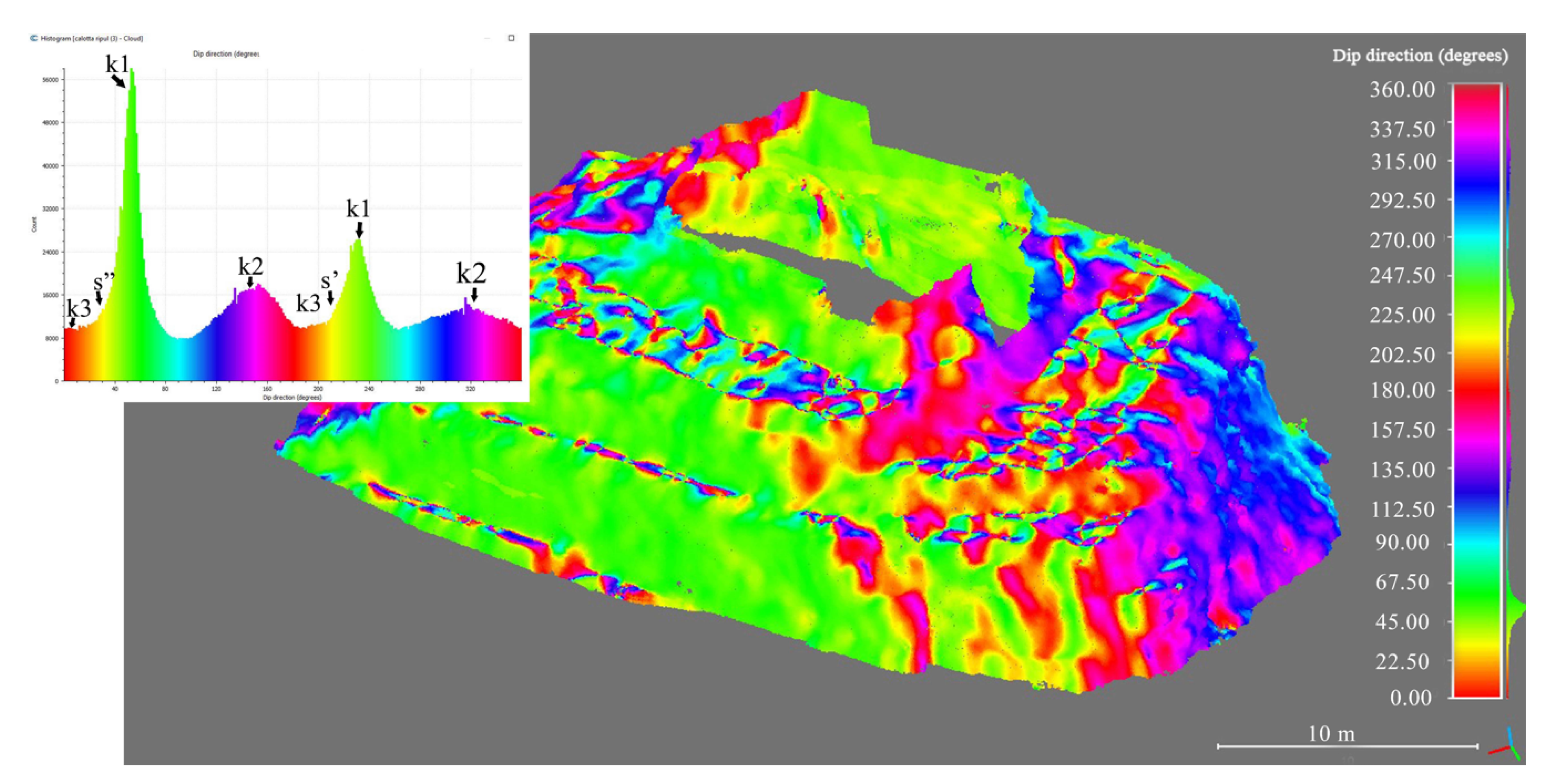
| Set | Dip Direction | Dip |
|---|---|---|
| K1 | 52 | 87 |
| K2 | 151 | 85 |
| K3 | 185 | 85 |
| S’ | 212 | 4 |
| S’’ | 35 | 3 |
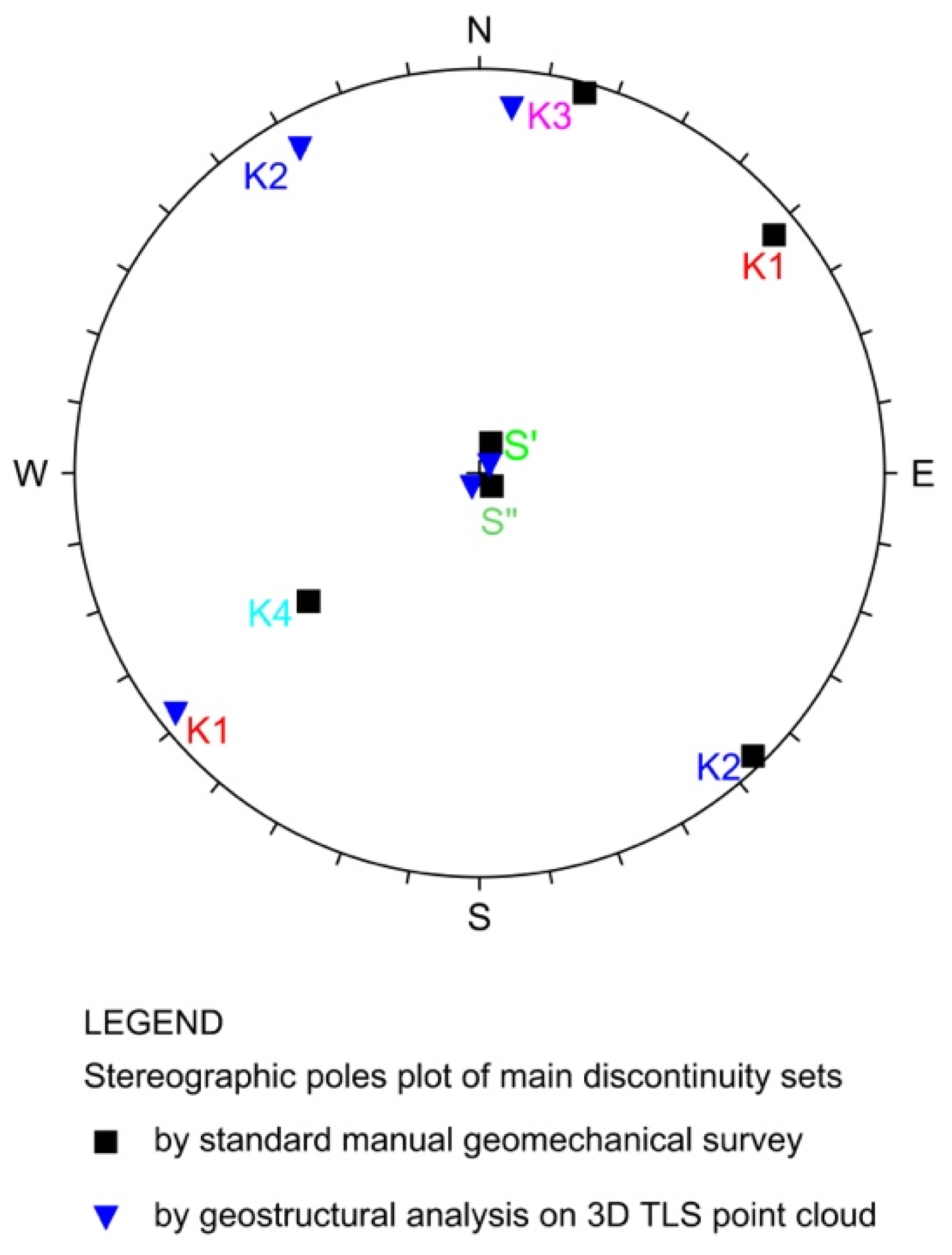
| Set | Dip Direction | Dip |
|---|---|---|
| K1 | 231 | 86 |
| K2 | 309 | 85 |
| K3 | 24 | 87 |
| K4 | 51 | 46 |
| S’ | 208 | 8 |
| S’’ | 333 | 6 |
© 2020 by the authors. Licensee MDPI, Basel, Switzerland. This article is an open access article distributed under the terms and conditions of the Creative Commons Attribution (CC BY) license (http://creativecommons.org/licenses/by/4.0/).
Share and Cite
Pagano, M.; Palma, B.; Ruocco, A.; Parise, M. Discontinuity Characterization of Rock Masses through Terrestrial Laser Scanner and Unmanned Aerial Vehicle Techniques Aimed at Slope Stability Assessment. Appl. Sci. 2020, 10, 2960. https://doi.org/10.3390/app10082960
Pagano M, Palma B, Ruocco A, Parise M. Discontinuity Characterization of Rock Masses through Terrestrial Laser Scanner and Unmanned Aerial Vehicle Techniques Aimed at Slope Stability Assessment. Applied Sciences. 2020; 10(8):2960. https://doi.org/10.3390/app10082960
Chicago/Turabian StylePagano, Marco, Biagio Palma, Anna Ruocco, and Mario Parise. 2020. "Discontinuity Characterization of Rock Masses through Terrestrial Laser Scanner and Unmanned Aerial Vehicle Techniques Aimed at Slope Stability Assessment" Applied Sciences 10, no. 8: 2960. https://doi.org/10.3390/app10082960
APA StylePagano, M., Palma, B., Ruocco, A., & Parise, M. (2020). Discontinuity Characterization of Rock Masses through Terrestrial Laser Scanner and Unmanned Aerial Vehicle Techniques Aimed at Slope Stability Assessment. Applied Sciences, 10(8), 2960. https://doi.org/10.3390/app10082960