Towards the Quantification of 5f Delocalization

Tobin, J. G.; Nowak, S.; Yu, S.-W.; Alonso-Mori, R.; Kroll, T.; Nordlund, D.; Weng, T.-C.; Sokaras, D.

doi:10.3390/app10082918

Open AccessFeature PaperArticle

Towards the Quantification of 5f Delocalization

¹

Departments of Physics and Chemistry, University of Wisconsin-Oshkosh, Oshkosh, WI 54901, USA

²

SLAC National Accelerator Laboratory, Menlo Park, CA 94025, USA

³

Lawrence Livermore National Laboratory, Livermore, CA 94550, USA

^*

Authors to whom correspondence should be addressed.

Appl. Sci. 2020, 10(8), 2918; https://doi.org/10.3390/app10082918

Submission received: 30 March 2020 / Revised: 14 April 2020 / Accepted: 18 April 2020 / Published: 23 April 2020

(This article belongs to the Special Issue Experimental and Theoretical Studies on the Physical Properties of Actinides and Their Oxides)

Download

Browse Figures

Versions Notes

Abstract

:

By using M_4,5 X-ray Emission Spectroscopy (XES) in the tender X-ray regime, it is possible to quantify 5f delocalization in the actinides. Previous analyses, utilizing the Branching Ratio (BR) in the N_4,5 X-ray Absorption Spectroscopy (XAS), could not discriminate between the cases of localized n = 2 and delocalized n = 3, in uranium materials, where n is the number of 5f electrons on the U entity. Here, it is shown that, by employing the ubiquitous 6p → 3d XES as a point of normalization, the localized n = 2 and delocalized n = 3 cases can be easily distinguished and quantified.

Keywords:

actinides; uranium; electronic structure

1. Introduction

X-ray spectroscopy has become a powerful tool for the analysis of the electronic structure of actinides, [1,2,3,4,5,6,7,8,9,10,11,12], based upon the original ground breaking work of (1) Veal and coworkers using X-ray Photoelectron Spectroscopy (XPS) [13,14,15,16]; (2) Naegele and others employing the lower energy Photoelectron Spectroscopy (PES) [17] and references therein; (3) Baer et al. utilizing Bremstrahlung Isochromat Spectroscopy (BIS) [18,19]; (4) Chauvet and Baptist, with the lower energy Inverse Photoelectron Spectroscopy (IPES) [20]; and Kalkowski, Kaindl, Brewer and Krone, who did a pioneering X-ray Absorption Spectroscopy (XAS) study [21].

A particularly effective approach has been to measure the Branching Ratios (BR) in the N_4,5 X-ray Absorption Spectroscopy, where BR = I_4d5/2 /(I_4d5/2 + I_4d3/2), I_x being the intensity of the respective level x. (Figure 1) The combination of strong electric dipole selection rules in the d to f transitions and a firm theoretical foundation for localized systems provided by van der Laan and Thole [22] has permitted the determination of the quantity of 5f electrons (n) in a number of localized actinide systems. While this may seem trivial, it was in fact a topic of serious disagreement for a number of years. For example, early on there was a viewpoint that championed 6d filling instead of 5f filling [23,24] and the reconciliation between the accepted n = 6 in atomic Pu and n = 5 in solid Pu was only realized completely in the recent past [25,26]. Nevertheless, there remained a very troublesome “fly in the ointment”: the indistinguishability of the BR for the localized n = 2 U systems and the delocalized n = 3 of uranium metal, as shown in Figure 2. This issue was first reported by Kalkowki, Kaindl, Brewer and Krone in 1987 [21] and addressed more recently elsewhere [27].

From other measurements and analyses, it has long been accepted that α-U has three 5f electrons and that there is significant delocalization in the 5f states [10,12,17,28]. An example of this is shown below in Figure 3. In Figure 3, the BIS of Baer et al. [18] is compared to the calculations of Kutepov [1,10,29]. The agreement between the BIS and the Unoccupied density of states (UDOS) derived from Kutepov’s calculations is very good. Moreover, the underlying j-specific calculations demonstrate the admixture of the 5f_5/2 and 5f_7/2 states, consistent with strong delocalization.

The essence of the problem is that the BR approach works very well for localized systems but cannot rule out the possibility of delocalization with a slightly different number of 5f electrons. However, there now appears to be a solution to this “blind spot.” Recently, it has been shown that the M_4,5 X-ray Emission Spectroscopy of UF₄ [30] exhibits results consistent with the Intermediate Coupling Model of van der Laan and Thole [22]. Normalizing to the 6p → 3d peaks, it can be seen that there is a tremendous differential in the intensities of the 5f peaks in the two spectra, a factor of 5. Figure 4 (The X-ray Emission Spectroscopy (XES) results for UO₂ are very similar to those of UF₄ [30] and are omitted here.) It has been shown that this is consistent with the almost pure n_5/2 nature of the two 5f electrons in UF₄ and strong, albeit not complete, adherence to electric dipole select rules. It will be demonstrated here that this type of data will provide (1) a direct pathway to the experimentally driven discernment of the localized n = 2 and delocalized n = 3 cases in particular and (2) the degree of delocalization in 5f systems in general.

2. Experimental

The X-ray Emission Spectroscopy experiments were done at the Stanford Synchrotron Radiation Lightsource, using Beamline 6-2a. These were performed utilizing both input photons from a Si(111) monochromator and a photon detector, a high-resolution Johansson-type spectrometer [31,32], operating in the tender X-ray regime (1.5–4.5 keV). For the UF₄ M₅ and UF₄ M₄ experiments, the excitation photon energies were, respectively, 3650 and 3820 eV. Each was chosen to be significantly above the threshold for the transition under consideration. Instrumentally, the total energy bandpass of this experiment is about 1 eV. However, the lifetime broadening of the 3d core holes (several eV) dominates the spectral widths. The sample used was the same as used in earlier studies [2,3]. Uranium samples can be affected by oxidation and sample corruption, but these were not a problem here, as described earlier [30].

3. Results and Discussion

Below, three problems will be addressed sequentially, using a single electron picture: (a) X-ray Absorption Spectroscopy (XAS) and the Branching Ratio (BR); (b) X-ray Emission Spectroscopy (XES) and the 5f:5f Peak Ratios; and (c) the 6p:5f Peak Ratios in XES. The prior success of the BR analysis in XAS, discussed briefly above, argues that the electric dipole selection rules work very well for the 4d → 5f transitions and that they should hold for 5f → 4d transitions as well. However, it will be seen that a correction term is required for the 5f → 3d transitions, which is not unexpected. The discussion will begin with the 4d-5f case, because the BR literature deals primarily with 4d → 5f transitions. For the XES, first, the 5f → 4d transitions will be considered, then the 5f → 3d transitions. The selection rules and cross sections are for d-f and should apply to all of these cases.

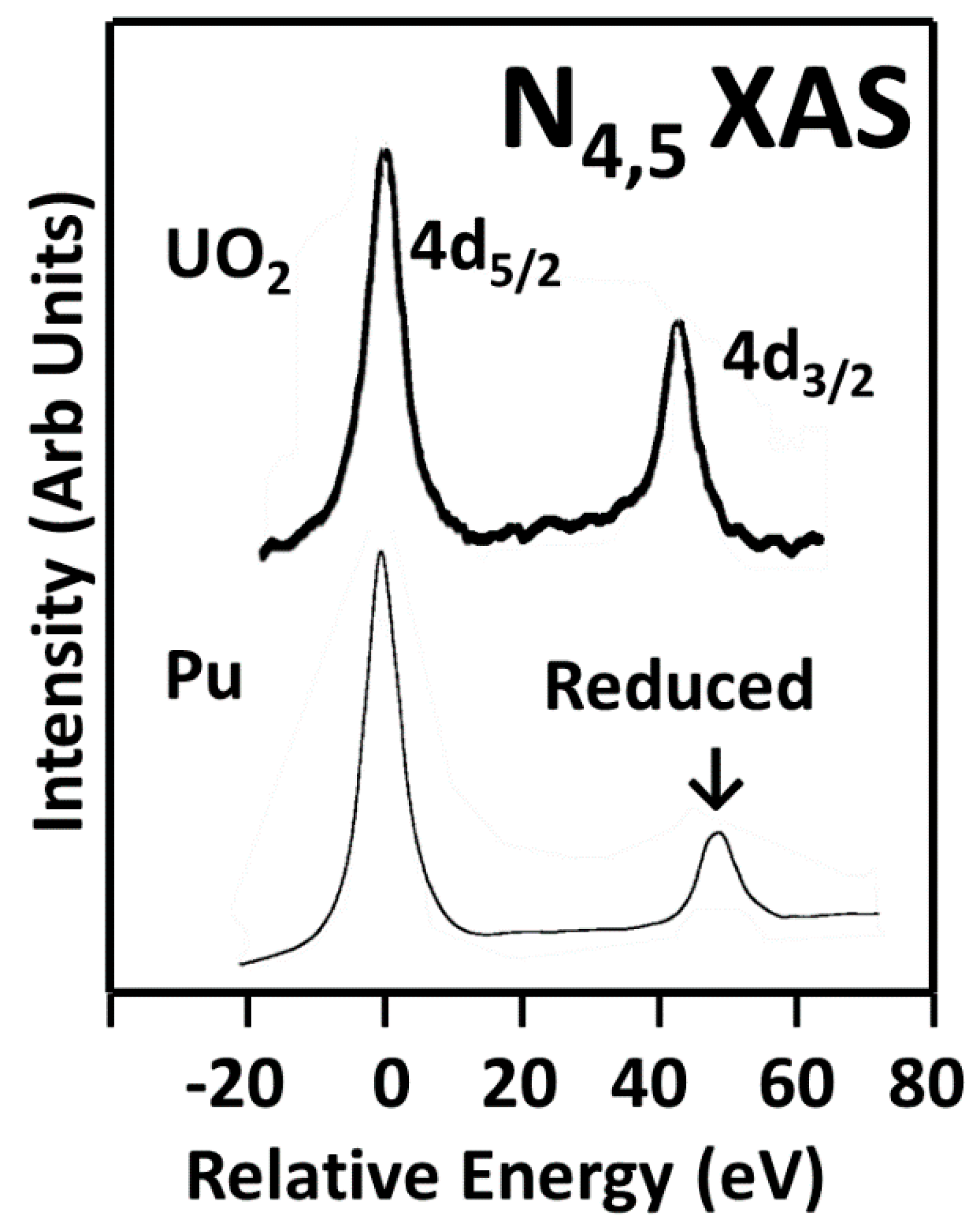
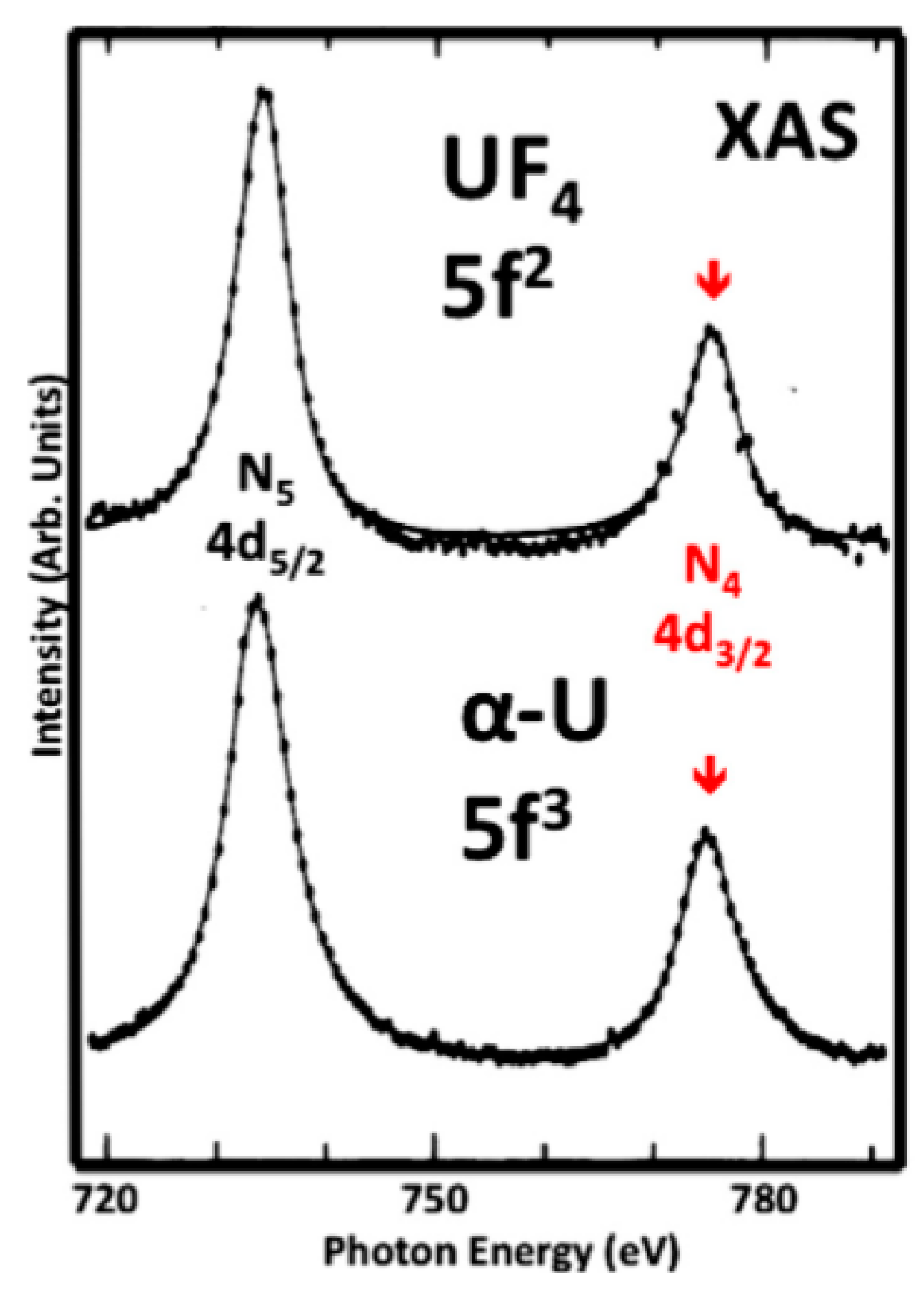
3.1. A Revisitation of XAS and the Branching Ratio

Let us begin by first considering the processes of X-ray Absorption Spectroscopy. Of course, van der Laan and Thole dealt with this in their earlier, ground-breaking work, including not just electric dipole transitions but also the intricacies of angular momentum for the three cases of Russell-Saunders or LS coupling, jj coupling and the Intermediate coupling case [22]. The goals here are more modest: to (1) better understand the underlying cause of the n = 2 localized/n = 3 delocalized dilemma and (2) to prepare to address the XES question.

The foundational single electron equations are below. A photon is absorbed and an electron moves from the 4d state into an empty 5f state. In Equation (1), there is only the 5f_5/2 final state. Under electric dipole selection rules, the transition into the 5f_7/2 state is forbidden. This selection rule, combined with preferentially filling the 5f_5/2 states, is the driving force behind the reduction in the 4d_3/2 peak in Pu, as seen in Figure 1 [10,11].

4d_3/2 + hv → 5f_5/2

(1)

4d_5/2 + hv → 5f_5/2 and 5f_7/2

(2)

If one applies the electric dipole operator to transitions between the states in the 4d manifolds [j =3/2 or 5/2, m_j> and the states in the 5f manifolds [j = 5/2 or 7/2, m_j>, one can obtain the relative cross sections shown in Table 1 [30,32]. Note that these cross sections are between completely filled 4d states and completely empty 5f states. (They would also apply for the reverse transitions, photon emission, between completely full 5f states and completely empty 4d states.)

However, the 5f states are NOT completely empty: the 5fs are partially occupied. The cross sections in Table 1 can be combined with the partial occupation to derive relative intensities, I_5/2 and I_3/2.

I_{\frac{5}{2}} = \frac{N_{5 / 2}}{6} (\frac{4}{15}) + \frac{N_{7 / 2}}{8} (\frac{80}{15})

(3)

I_{\frac{3}{2}} = \frac{N_{5 / 2}}{6} (\frac{56}{15})

(4)

B R = \frac{I_{\frac{5}{2}}}{I_{\frac{5}{2}} + I_{\frac{3}{2}}} = (\frac{1}{15}) (\frac{N_{5 / 2}}{N}) + (\frac{N_{7 / 2}}{N}) = 1 - (\frac{14}{15}) (\frac{N_{5 / 2}}{N})

(5)

where N is the total number of 5f holes, N_5/2 is the number of holes in the 5f_5/2 manifold and N_7/2 is the number of holes in the 5f_7/2 manifold. Obviously, N = N_{5/2 +} N_7/2 and n = 14 − N, n_5/2 = 6 − N_5/2 and n_7/2 = 8 − N_7/2, where n_x is the corresponding number of electrons in each 5f manifold. If the appropriate filling pattern is used for each case, Equation (5) can generate the correct branching ratio for every case and equation in Table 1 in Reference [10], including the statistical, jj and intermediate cases as well as the experimental values. This then brings the discussion back to the degeneracy of the n = 2 localized case and the n = 3 delocalized case. While the two cases have significantly different occupations, they both have the same percentage un-occupations in the 5/2 and 7/2 manifolds of the 5f states. (Table 2) This suggests that a technique that was dependent upon occupation, not un-occupations, would be able to differentiate the two cases. Such techniques would include X-ray Emission Spectroscopy between the 5f and 4d or 3d manifolds. That will be considered next.

Values extracted from [2,10] and the equations above.

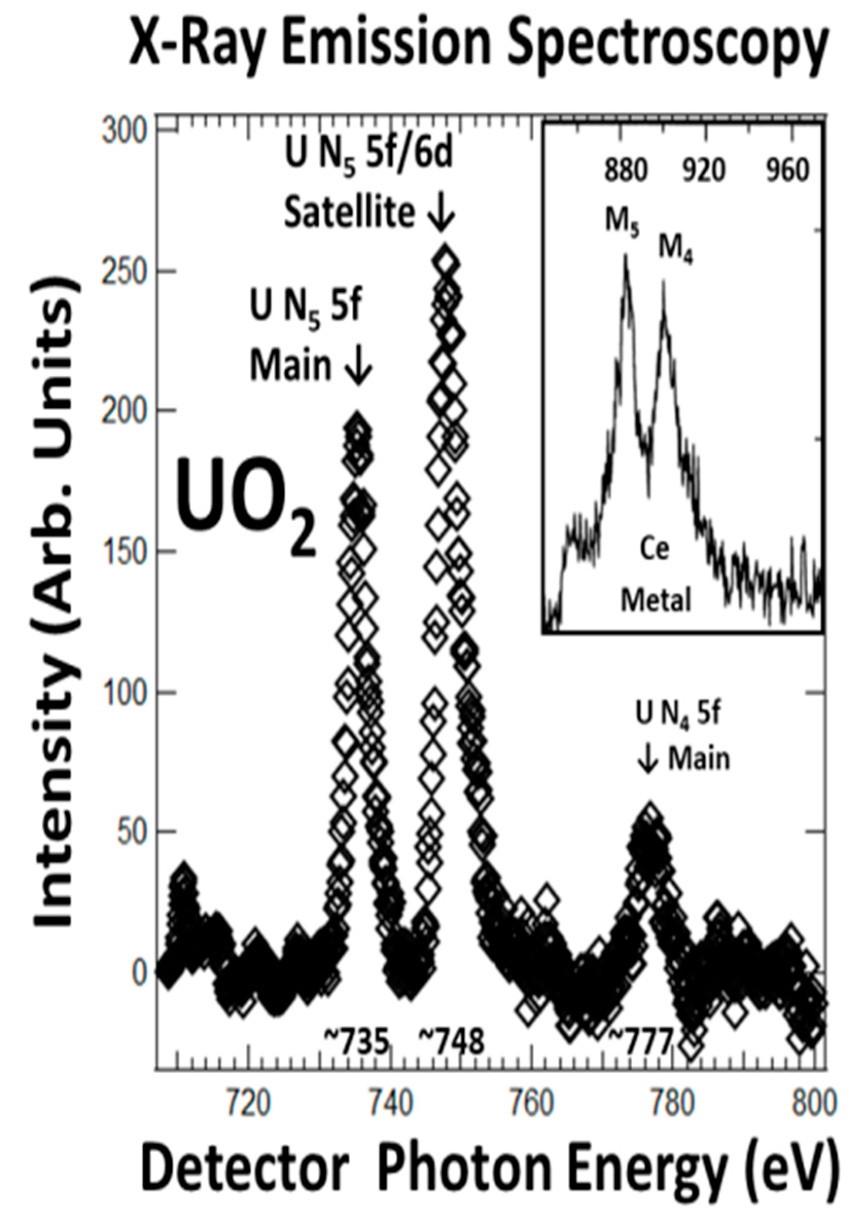
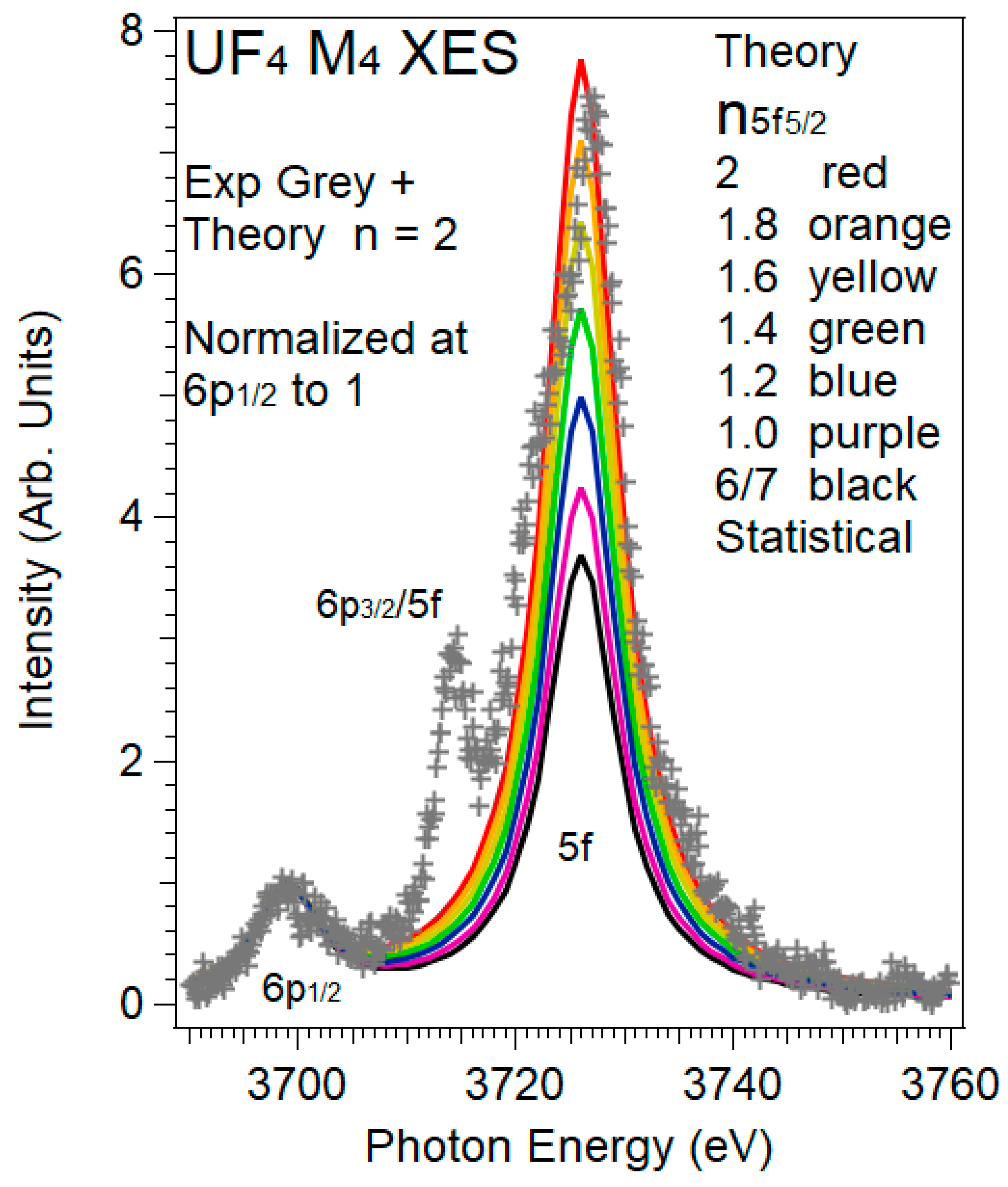
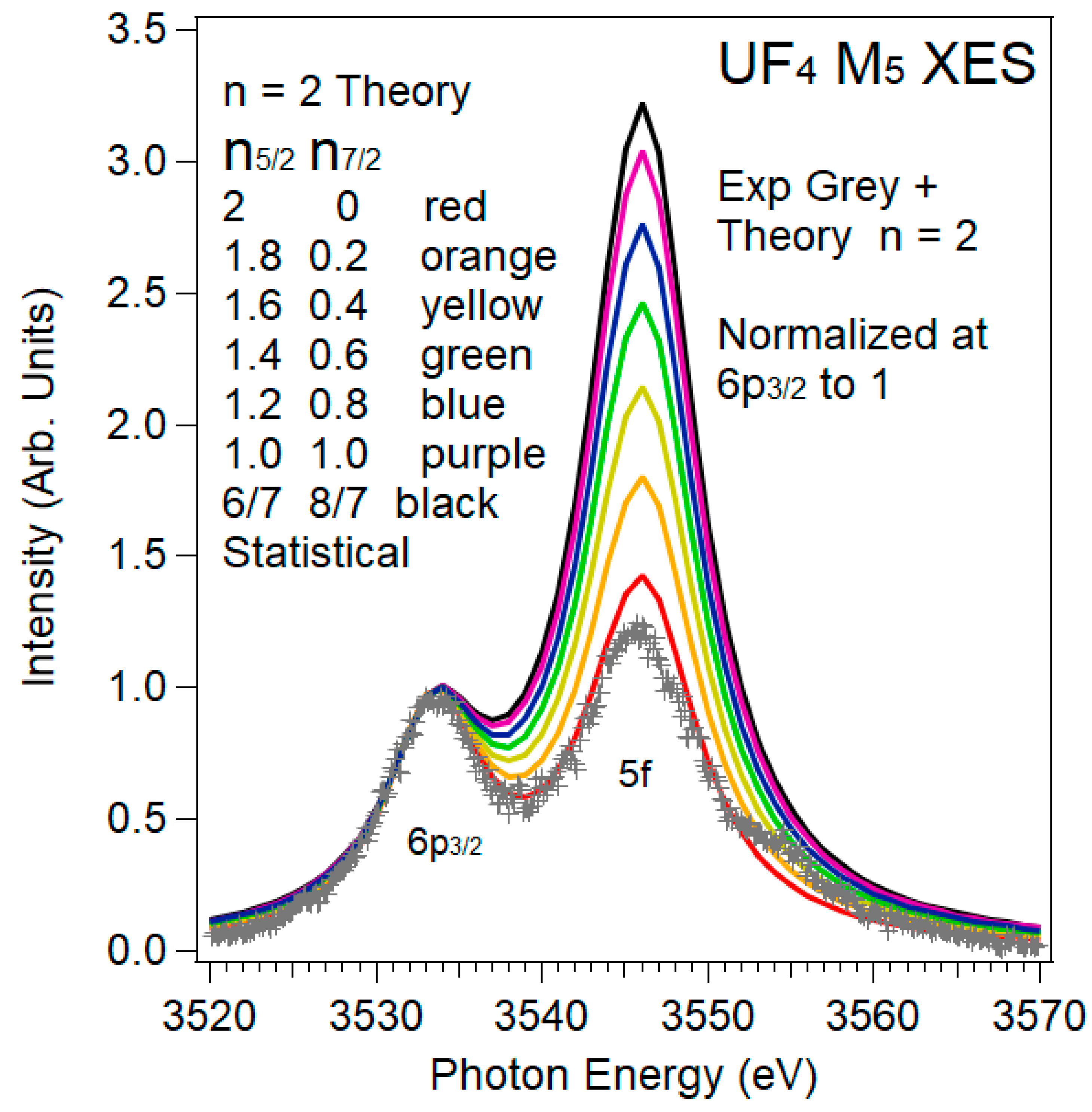
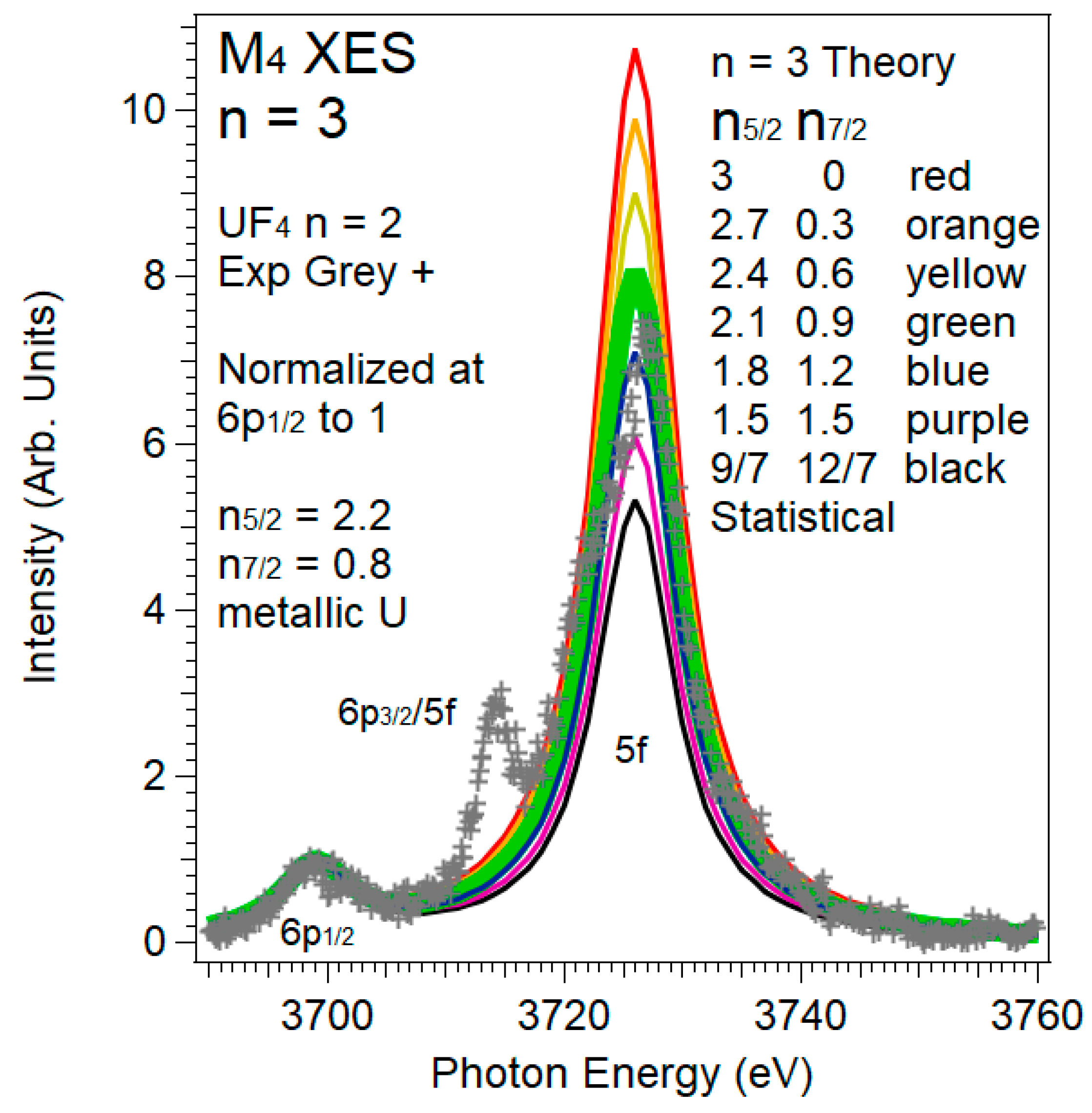
3.2. XES and 5f:5f Peak Ratios

It is possible to apply a parallel analysis to X-ray Emission Spectroscopy. The cross sections are closely related, as seen in Table 3, but now there is a partial occupation of the 5f states as before but only one hole in the d level.

From these, it is possible to calculate relative intensities and a Peak Ratio (PR).

I_{5 f}^{N 5} = \frac{n_{5 / 2}}{6} (\frac{4}{90}) + \frac{n_{7 / 2}}{8} (\frac{16}{18})

(6)

I_{5 f}^{N 4} = \frac{n_{5 / 2}}{6} (\frac{56}{60})

(7)

P R = \frac{I_{5 f}^{N 4}}{I_{5 f}^{N 5}} = \frac{(\frac{n_{5 / 2}}{6}) (\frac{56}{60})}{(\frac{n_{5 / 2}}{6}) (\frac{4}{90}) + (\frac{n_{7 / 2}}{8}) (\frac{16}{18})} = \frac{21 n_{5 / 2}}{(n_{5 / 2}) + (15 n_{7 / 2})}

(8)

Now, consider some limiting case behavior. In the ultimate limit, the material would be pure n_5/2: n = n_5/2, n_7/2 = 0 and PR = 21. This would require a jj coupling and has not been observed experimentally. Experimentally, UO₂ is an example of localized case with a strong spin-orbit splitting. For UO₂, it is n = 2, n_5/2 = 1.96 and n_7/2 = 0.04, from Table 2 above. From Equation (8), the result would be PR (UO₂) = 16. From the data in Figure 5 [33], the ratio of the N4: N5 intensity is 9, although the situation is complicated by the presence a very strong satellite. (It is not clear that the satellite and main peaks would have the same cross sectional dependences.) Nevertheless, there is a qualitative, perhaps even semi-quantitative confirmation of Equation (8).

Another limiting case would be a small spin-orbit splitting with a statistical distribution of electrons in the f states. Ce metal is a good approximation to this limiting case, with n = 1, a small spin-orbit splitting and significant delocalization, which tends to mix the 4f_5/2 and 4f_7/2 states even further. (Ce is a 4f material and the transitions would be 4f → 3d, but the dependences should be the same. The 4f splitting of the Rare Earths is significantly smaller than the 5f splitting of the actinides [27]). The M_4,5 spectrum of Ce metal is shown in the inset in Figure 5 [34,35]. The predicted PR for the statistical distribution (n_5/2/n_7/2 = ¾) would be 1. As can be seen in the inset in Figure 5, the M₄ and M₅ intensities are approximately equal based upon peak heights.

These two limiting cases provide a significant confirmation of Equations (6)–(8), with an order of magnitude variation in the PRs of these two limits. On the other hand, as reported earlier [30], the measured peak ratio for the M_4,5 XES of UF₄ is only ~5, down a factor of two from the N_4,5 results for UO₂. Both UO₂ and UF₄ are highly localized, n = 2 cases [2] with BR values of 0.68 each and with the M₅ XES spectra of UO₂ and UF₄ being very similar [30]. Thus, it is expected that the UO₂ and UF₄ results should be similar if not identical. However, the discrepancy between U N_4,5 and U M_4,5 results is not unanticipated. It is reasonable to expect that the U N_4,5 (and Ce M_4,5) situation would fall inside the long wavelength approximation used in the derivation of the electric dipole approximation [36,37]. The stunning success of the body of work based upon the application of the Intermediate Coupling Model to the experimentally measured N_4,5 BRs supports this contention strongly [3,10,11,12]. Nevertheless, the higher energies of the U N_4,5 transitions mean shorter photon wavelengths, which translates into a larger impact for the higher order terms, such as magnetic dipole and electric quadrupole [30].

Empirically, it is possible to correct for these higher order terms by adding a term to the numerator and denominator in Equation (8). Because the PR is being reduced and the denominator value is much smaller than the numerator, it is reasonable to begin by adding a corrective term to the denominator only.

P R = \frac{I_{5 f}^{M 4}}{I_{5 f}^{M 5}} = \frac{21 n_{5 / 2}}{(n_{5 / 2}) + (15 n_{7 / 2}) + a}

(9)

Plugging in the values for UF₄ (PR = 4.6), the following value is found: a ≈ 6.4. Assuming that “a” is a constant, the following equation is obtained.

P R = \frac{21 n_{5 / 2}}{(n_{5 / 2}) + (15 n_{7 / 2}) + 6.4}

(10)

For the two cases in Table 2, the simple model would predict these PRs: PR (UF₄) ≈ 5 and PR (U metal) ≈ 2.3. Obviously, it will be possible to easily distinguish these two cases with M_4,5 XES. However, owing to the large separation between the M₄ and M₅ edges in U, the spectra are collected separately and then normalized through the accompanying 6p XES, as can be seen in Figure 4. Thus, the best approach is to build the model around the 6p normalization. This issue will be addressed next.

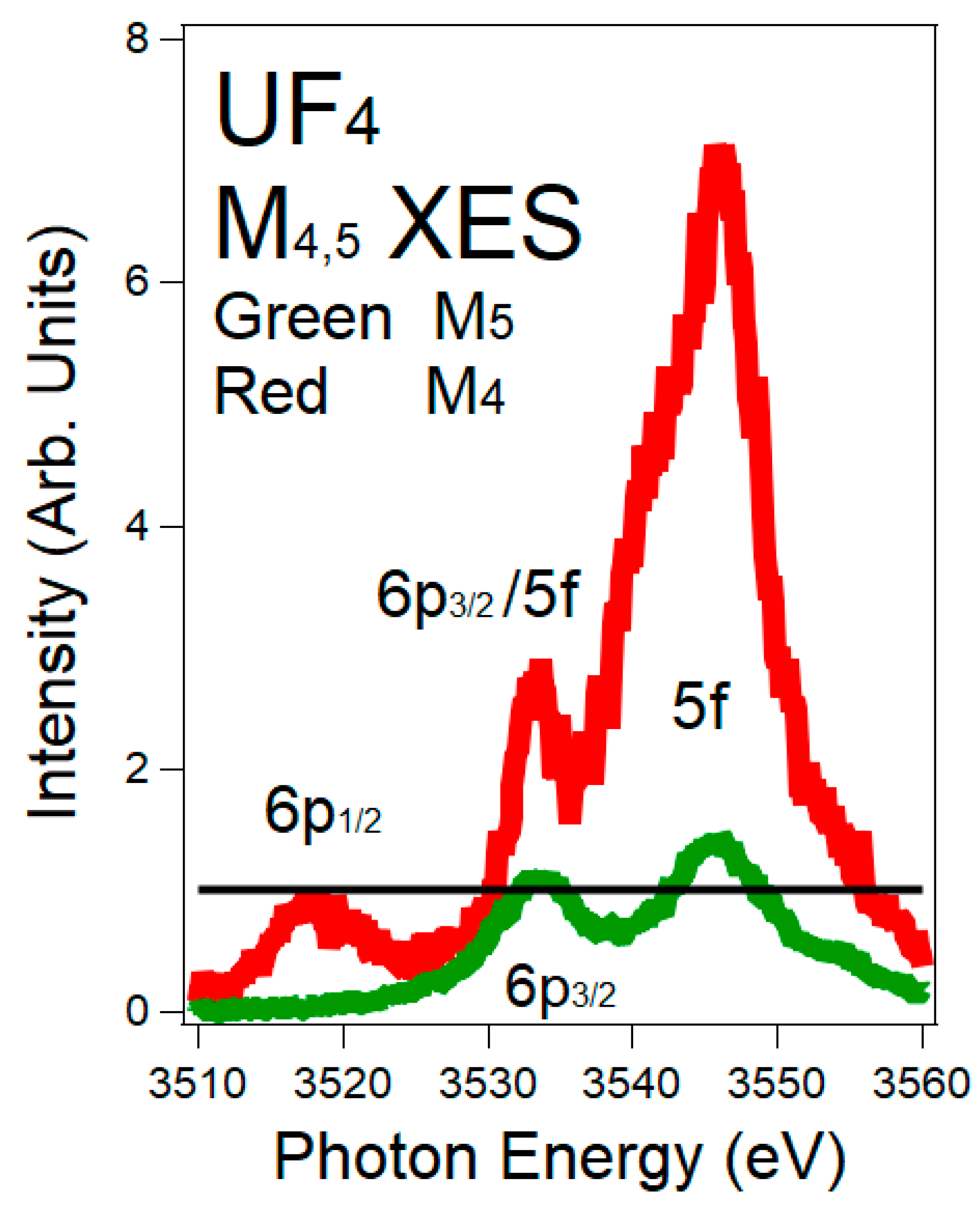
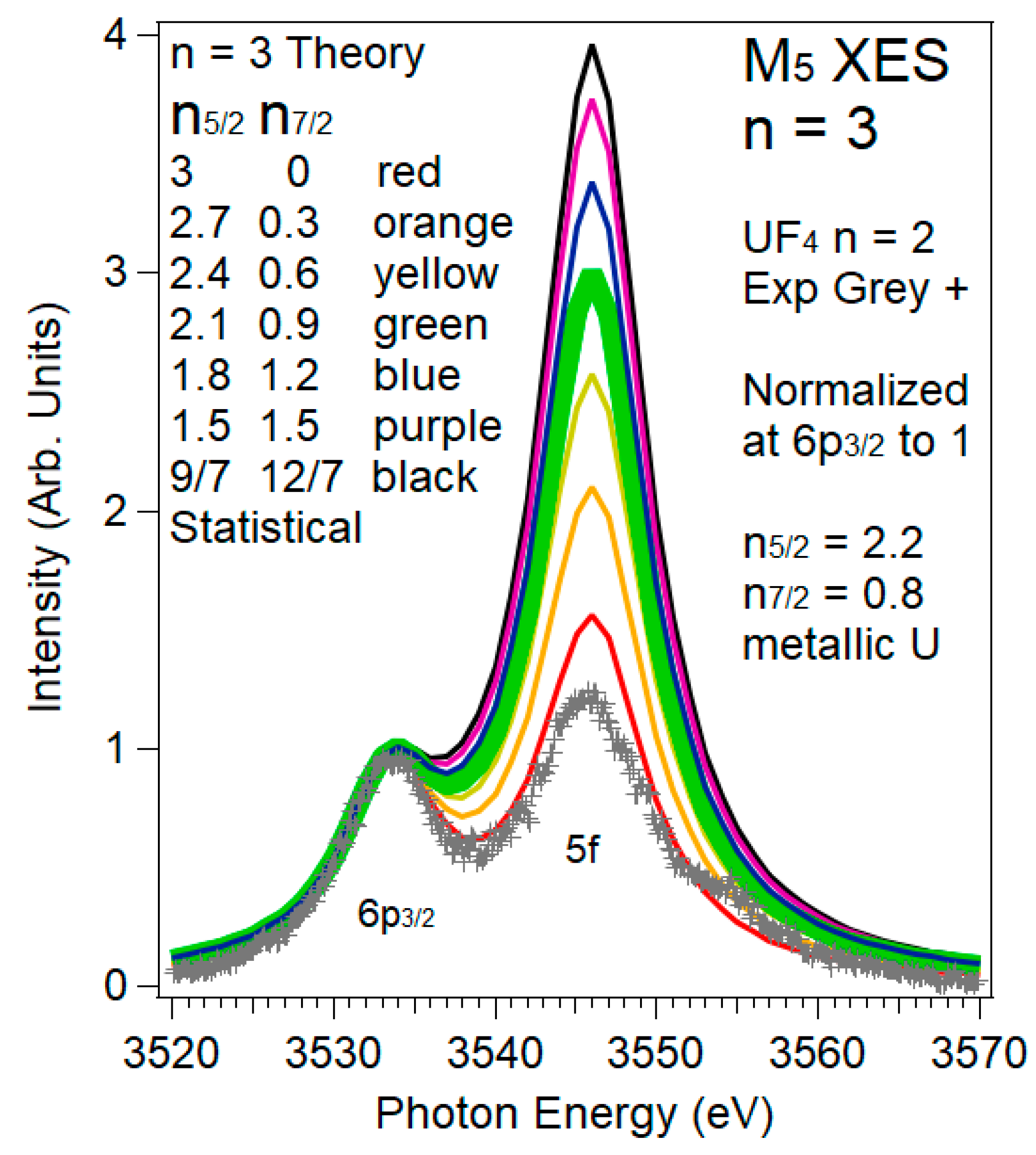
3.3. XES and 5f:6p Peak Ratios

It is possible to calculate the electric dipole relative cross sections for the 6p → 3d transitions, following the same procedures as discussed earlier for the 5f → 3d transitions. The results are shown in Table 4 [30]. In this case, the 6ps are completely full and, because the 6ps should sit inside the 5f’s [30], the electric dipole selection rules and cross sections should hold. One piece of information supporting this assertion is the absence of the 6p_1/2 peak in the M₅ spectrum in Figure 4, consistent with the cross section of zero in Table 4. For the 6p → 3d transitions, the Δj = +1 transitions are the strongest and will be utilized for the normalization of the 5f intensities to the 6p intensities. At this point, it is possible to write out the relative intensity equations, including some constants for effects, such as the radial matrix elements.

I_{5 f}^{M 4} = C_{5 f} {\frac{n_{5 / 2}}{6} (\frac{56}{60})}

(11)

I_{5 f}^{M 5} = C_{5 f} {\frac{n_{5 / 2}}{6} (\frac{4}{90}) + \frac{n_{7 / 2}}{8} (\frac{16}{18}) + \frac{6.4}{135}}

(12)

I_{6 p_{1 / 2}}^{M 4} = C_{6 p} (\frac{1}{3})

(13)

I_{6 p_{3 / 2}}^{M 5} = C_{6 p} (\frac{2}{5})

(14)

P R_{f p}^{M 4} = \frac{I_{5 f}^{M 4}}{I_{6 p_{1 / 2}}^{M 4}} = (\frac{C_{5 f}}{C_{6 p}}) {\frac{(\frac{n_{5 / 2}}{6}) (\frac{56}{60})}{(\frac{1}{3})}}

(15)

P R_{f p}^{M 5} = \frac{I_{5 f}^{M 5}}{I_{6 p_{3 / 2}}^{M 5}} = (\frac{C_{5 f}}{C_{6 p}}) {\frac{\frac{n_{5 / 2}}{6} (\frac{4}{90}) + \frac{n_{7 / 2}}{8} (\frac{16}{18}) + \frac{6.4}{135}}{(\frac{2}{5})}}

(16)

From the UF₄ experimental results [30], it is possible to determine (C_5f/C_6p).

{(P R_{f p}^{M 4})}_{U F_{4}}^{E x p} = 10.4 \to (\frac{C_{5 f}}{C_{6 p}}) = 11.34

(17)

Finally, substituting, the equations become as follows:

P R_{f p}^{M 4} = \frac{I_{5 f}^{M 4}}{I_{6 p_{1 / 2}}^{M 4}} = 5.31 n_{5 / 2}

(18)

P R_{f p}^{M 5} = \frac{I_{5 f}^{M 5}}{I_{6 p_{3 / 2}}^{M 5}} = 0.2098 n_{5 / 2} + 3.150 n_{7 / 2} + 1.361

(19)

Setting n = 2 and applying Equations (16) and (17), the results in Figure 6 and Figure 7 were generated. Here, the spectra are normalized to a value of one at the 6p maximum, as shown below. Note the strong agreement of the experiment and the n_5/2 = 2 curve in each, as expected.

The real point of this exercise is not to confirm the analysis for the localized n = 2 case but rather to project what the n = 3 delocalized case would be. To that end, setting n = 3 and applying the equations again, the plots in Figure 8 and Figure 9 were obtained.

Interestingly, the M₄ spectrum corresponding to the n = 3, delocalized case (n_5/2 = 2.1, Green or possibly n_5/2 = 2.4, yellow) is not substantially different to the experimental spectrum for the n = 2 localized case, the UF₄ result. This is because the n_5/2 value for the delocalized n =3 case would only be about n_5/2 = 2.23, not very different from the n = 2 localized case. (Table 2) One the other hand, the M₅ projection shows a very clear and substantial change. The n_5/2 = 2.1 (green) spectrum, and even the n_5/2 = 2.4 (yellow), are very different to the experimental M₅ spectrum for UF₄. This is because the major change in the delocalization is to significantly populate the n_7/2 states, which in turn is manifested in the M₅ spectrum, not the M₄.

4. Summary and Conclusions

By using M_4,5 X-ray Emission Spectroscopy (XES) in the tender X-ray regime, it has been shown that it is possible to quantify 5f delocalization in the actinides. Previous analyses, utilizing the Branching Ratio (BR) in the N_4,5 X-ray Absorption Spectroscopy (XAS), could not discriminate between the cases of localized n = 2 and delocalized n = 3, in uranium materials, where n is the number of 5f electrons on the U entity. Here it is shown that, by employing the ubiquitous 6p XES as a point of normalization, the localized n = 2 and delocalized n = 3 cases can be easily distinguished and quantified via the M₅ X-ray emission spectrum.

As can be seen from the Introduction, XAS, XES, BIS and XPS each provide different types of information. Of course, all spectroscopies provide a measure of the joint density of states of the initial and final manifolds, connected by the appropriate operator. BIS and XPS can give a picture of the unoccupied and occupied DOS of a material, respectively, generally without elemental specificity but possibly with linear (translational) momentum resolution [38,39,40]. On the other hand, XAS and XES provide information about the unoccupied and occupied DOS, respectively, but with elemental and generally angular momentum resolution. In the case of the 5f states, the XES and XAS of the d-f transitions can provide a measure of the 5f state occupations, including a breakdown into the 5f_5/2 and 5f_7/2 distributions. The discussions today have been made within the framework of the n = 3 delocalization problem for metallic U. However, there are also other perturbations that can mix the 5f_5/2 and 5f_7/2 states, e.g., magnetic effects [41] and crystal field effects [42]. XES and XAS together should produce a measure of the magnitude of the number and distribution of the 5f electrons, but to assign the distribution as being due to delocalization will require a demonstration that other mixing effects are not significantly in effect. Obvously, all of this is played out under the conditions of the competition between angular momentum and delocalization effects, i.e., 5f duality [10,43,44].

Author Contributions

All authors provided crucial and essential support to the experiment and analysis. S.N., R.A.-M., T.K., D.N., T.-C.W. and D.S. designed, assembled, implemented and commissioned the high resolution detection system and beamline. S.N. and D.S. handled the samples, collected the SLAC data and performed very sophisticated data reduction. S.-W.Y. collected and analyzed the offsite data. J.G.T. provided the uranium fluoride sample, performed further data analysis and led the manuscript preparation, with particularly crucial input from D.S. All authors have read and agreed to the published version of the manuscript.

Funding

This research was funded by Department of Energy, under Contract No. DE-AC02-05CH11231 and DE-AC52-07NA27344, as described below. The Article Publication Charge was waived.

Acknowledgments

Stanford Synchrotron Radiation Light-source is a national user facility operated by Stanford University on behalf of the DOE and the OBES. Part funding for the instrument used for this study came from the U.S. Department of Energy, Office of Energy Efficiency & Renewable Energy, Solar Energy Technology Office BRIDGE Program. Resources of the National Energy Research Scientific Computing Center, a DOE Office of Science User Facility supported by the Office of Science of the U.S. Department of Energy under Contract No. DE-AC02-05CH11231, were used in this work. LLNL is operated by Lawrence Livermore National Security, LLC, for the U.S. Department of Energy, National Nuclear Security Administration, under Contract DE-AC52-07NA27344. The authors also wish to thank E. Bauer of LANL and C. Booth of LBNL for their help with this work.

Conflicts of Interest

The authors declare no conflict of interest. The funders had no role in the design of the study; in the collection, analyses, or interpretation of data; in the writing of the manuscript, or in the decision to publish the results.

References and Note

Tobin, J.G.; Shuh, D.K. Electron spectroscopy of the oxidation and aging of U and Pu. J. Electron. Spectrosc. Relat. Phenom. 2015, 205, 83. [Google Scholar] [CrossRef] [Green Version]
Tobin, J.G.; Yu, S.-W.; Booth, C.H.; Tyliszczak, T.; Shuh, D.K.; van der Laan, G.; Sokaras, D.; Nordlund, D.; Weng, T.-C.; Bagus, P.S. Oxidation and crystal field effects in uranium. Phys. Rev. B 2015, 92, 035111. [Google Scholar] [CrossRef] [Green Version]
Tobin, J.G.; Yu, S.-W.; Qiao, R.; Yang, W.L.; Booth, C.H.; Shuh, D.K.; Duffin, A.M.; Sokaras, D.; Nordlund, D.; Weng, T.-C. Covalency in oxidized uranium. Phys. Rev. B 2015, 92, 045130. [Google Scholar] [CrossRef] [Green Version]
Booth, C.H.; Jiang, Y.; Wang, D.L.; Mitchell, J.N.; Tobash, P.H.; Bauer, E.D.; Wall, M.A.; Allen, P.G.; Sokaras, D.; Nordlund, D.; et al. Multiconfigurational nature of 5f orbitals in uranium and plutonium intermetallics. Proc. Natl. Acad. Sci. USA 2012, 109, 10205–10209. [Google Scholar] [CrossRef] [Green Version]
Booth, C.H.; Medling, S.A.; Jiang, Y.U.; Bauer, E.D.; Tobash, P.H.; Mitchell, J.N.; Veirs, D.K.; Wall, M.A.; Allen, P.G.; Kas, J.J.; et al. Delocalization and occupancy effects of 5f orbitals in plutonium intermetallics using L₃-edge resonant X-ray emission spectroscopy. J. Electron. Spectrosc. Relat. Phenom. 2014, 194, 57. [Google Scholar] [CrossRef] [Green Version]
Booth, C.H.; Medling, S.A.; Tobin, J.G.; Baumbach, R.E.; Bauer, E.D.; Sokaras, D.; Nordlund, D.; Weng, T.C. Probing 5f-state configurations in URu₂Si₂ with U L_III-edge resonant x-ray emission spectroscopy. Phys. Rev. B 2016, 94, 045121. [Google Scholar] [CrossRef] [Green Version]
Kvashnina, K.O.; Butorin, S.M.; Martin, P.; Glatzel, P. Chemical State of Complex Uranium Oxides. Phys. Rev. Lett. 2013, 111, 253002. [Google Scholar] [CrossRef] [Green Version]
Vitova, T.; Pidchenko, I.; Fellhauer, D.; Bagus, P.S.; Joly, Y.; Pruessmann, T.; Bahl, S.; Gonzalez-Robles, E.; Rothe, J.; Altmaier, M.; et al. The role of the 5f valence orbitals of early actinides in chemical bonding. Nat. Comm. 2017, 8, 16053. [Google Scholar] [CrossRef]
Tobin, J.G.; Yu, S.-W. Orbital Specificity in the Unoccupied States of UO₂ from Resonant Inverse Photoelectron Spectroscopy. Phys. Rev. Lett. 2011, 107, 167406. [Google Scholar] [CrossRef] [Green Version]
Tobin, J.G.; Moore, K.T.; Chung, B.W.; Wall, M.A.; Schwartz, A.J.; van der Laan, G.; Kutepov, A.L. Competition between delocalization and spin-orbit splitting in the actinide 5f states. Phys. Rev. B 2005, 72, 085109. [Google Scholar] [CrossRef]
van der Laan, G.; Moore, K.T.; Tobin, J.G.; Chung, B.W.; Wall, M.A.; Schwartz, A.J. Applicability of the Spin-Orbit Sum Rule for the Actinide 5f States. Phys. Rev. Lett. 2004, 93, 097401. [Google Scholar] [CrossRef]
Moore, K.T.; Wall, M.A.; Schwartz, A.J.; Chung, B.W.; Shuh, D.K.; Schulze, R.K.; Tobin, J.G. Failure of Russell-Saunders Coupling in the 5f States of Plutonium. Phys. Rev. Lett. 2003, 90, 196404. [Google Scholar] [CrossRef]
Veal, B.W.; Lam, D.J.; Diamond, H.; Hoekstra, H.R. X-ray photoelectron-spectroscopy study of oxides of the transuranium elements Np, Pu, Am, Cm, Bk, and Cf. Phys. Rev. B 1977, 15, 2929. [Google Scholar] [CrossRef]
Veal, B.W.; Lam, D.J.; Carnall, W.T.; Hoekstra, H.R. X-ray photoemission spectroscopy study of hexavalent uranium compounds. Phys. Rev. B 1975, 12, 5651. [Google Scholar] [CrossRef]
Veal, B.W.; Lam, D.J. X-ray photoelectron studies of thorium, uranium, and their dioxides. Phys. Rev. B 1974, 10, 4902. [Google Scholar] [CrossRef]
Veal, B.W.; Lam, D.J. Bonding in uranium oxides: The role of 5f electrons. Phys. Lett. 1974, 49A, 466–468. [Google Scholar] [CrossRef]
Naegele, J.R. Actinides and some of their alloys and compounds, Electronic Structure of Solids: Photoemission Spectra and Related Data, Landolt-Bornstein Numerical Data and Functional Relationships in Science and Technology, ed. A Goldmann Group III 1994, 23, 183–327. [Google Scholar]
Baer, Y.; Lang, J.K. High-energy spectroscopic study of the occupied and unoccupied 5f and valence states in Th and U metals. Phys. Rev. B 1980, 21, 2060. [Google Scholar] [CrossRef]
Baer, Y.; Schoenes, J. Electronic structure and Coulomb correlation energy UO2 single crystal. Solid State Commun. 1980, 33, 885. [Google Scholar] [CrossRef]
Chauvet, G.; Baptist, R. Inverse photoemission study of uranium dioxide. Solid State Commun. 1982, 43, 793. [Google Scholar] [CrossRef]
Kalkowski, G.; Kaindl, G.K.; Brewer, W.D.; Krone, W. Near-edge x-ray-absorption fine structure in uranium compounds. Phys. Rev. B 1987, 35, 2667–2677. [Google Scholar] [CrossRef] [Green Version]
van der Laan, G.; Thole, B.T. X-ray-absorption sum rules in jj-coupled operators and ground-state moments of actinide ions. Phys. Rev. B 1996, 53, 14458. [Google Scholar] [CrossRef]
Zachariasen, W.H. Metallic radii and electron configurations of the 5f−6d metals. J. Inorg. Nucl. Chem. 1973, 35, 3487. [Google Scholar] [CrossRef]
Skriver, H.L.; Andersen, O.K.; Johansson, B. Calculated Bulk Properties of the Actinide Metals. Phys. Rev. Lett. 1978, 41, 42. [Google Scholar] [CrossRef]
Ryzhkov, M.V.; Mirmelstein, A.; Yu, S.-W.; Chung, B.W.; Tobin, J.G. Probing actinide electronic structure through pu cluster calculations. Int. J. Quantum Chem. 2013, 113, 1957. [Google Scholar] [CrossRef]
Ryzhkov, M.V.; Mirmelstein, A.; Delley, B.; Yu, S.-W.; Chung, B.W.; Tobin, J.G. The Effects of Mesoscale Confinement in Pu Clusters. J. Electron. Spectrosc. and Relat. Phenom. 2014, 194, 45. [Google Scholar] [CrossRef]
Tobin, J.G. The apparent absence of chemical sensitivity in the X-ray absorption spectroscopy of uranium compounds. J. Electron. Spectrosc. Relat. Phenom. 2014, 194, 14. [Google Scholar] [CrossRef]
Opeil, C.P.; Schulze, R.K.; Volz, H.M.; Lashley, J.C.; Manley, M.E.; Hults, W.L.; Hanrahan, R.J., Jr.; Smith, J.L.; Mihaila, B.; Blagoev, K.B.; et al. Angle-resolved photoemission and first-principles electronic structure of single-crystalline α-U(001). Phys. Rev. B 2007, 75, 045120. [Google Scholar] [CrossRef] [Green Version]
Butterfield, M.T.; Tobin, J.G.; Teslich, N.E., Jr.; Bliss, R.A.; Wall, M.A.; McMahan, A.K.; Chung, B.W.; Schwartz, A.J.; Kutepov, A.L. Utilizing Nano-focussed Bremstrahlung Isochromat Spectroscopy (nBIS) to Determine the Unoccupied Electronic Structure of Pu. Matl. Res. Soc. Symp. Proc. 2006, 893, 95. [Google Scholar]
Tobin, J.G.; Nowak, S.; Yu, S.-W.; Alonso-Mori, R.; Kroll, T.; Nordlund, D.; Weng, T.-C.; Sokaras, D. Observation of 5f intermediate coupling in uranium x-ray emission spectroscopy. J. Phys. Commun. 2020, 4, 015013. [Google Scholar] [CrossRef]
Nowak, S.H.; Armenta, R.; Schwartz, C.P.; Gallo, A.; Abraham, B.; Garcia-Esparza, A.T.; Biasin, E.; Prado, A.; Maciel, A.; Zhang, D.; et al. A versatile Johansson-type tender x-ray emission spectrometer. Rev. Sci. Instrum. 2020, 91, 033101. [Google Scholar] [CrossRef] [PubMed]
Tobin, J.G.; Nowak, S.; Booth, C.H.; Bauer, E.D.; Yu, S.-W.; Alonso-Mori, R.; Kroll, T.; Nordlung, D.; Weng, T.-C.; Sokaras, D. Separate Measurement of the 5f5/2 and 5f7/2 Unoccupied Density of States of UO₂. J. Electron. Spectrosc. Relat. Phenom. 2019, 232, 100. [Google Scholar] [CrossRef] [Green Version]
Yu, S.-W.; Tobin, J.G. Multi-electronic effects in uranium dioxide from X-ray Emission Spectroscopy. J. Electron. Spectrosc. Relat. Phenom. 2013, 187, 15. [Google Scholar] [CrossRef]
Tobin, J.G.; Yu, S.W.; Chung, B.W.; Waddill, G.D.; Duda, L.; Nordgren, J. Observation of strong resonant behavior in the inverse photoelectron spectroscopy of Ce oxide. Phys. Rev. B 2011, 83, 085104. [Google Scholar] [CrossRef] [Green Version]
Courtesy of Emiliana Damian, L. Duda, and J. Nordgren. Please see Ref. [34].
Gottfried, K. Quantum Mechanics, Volume I: Fundamentals; Benjamin-Cummings: Reading, MA, USA, 1966. [Google Scholar]
Cohen-Tannoudji, C.; Diu, B.; Laloë, F. Quantum Mechanics; Wiley: New York, NY, USA, 1973; Volumes I & II. [Google Scholar]
Fujimori, S.-I.; Kobata, M.; Takeda, Y.; Okane, T.; Saitoh, Y.; Fujimori, A.; Yamagami, H.; Haga, Y.; Yamamoto, E.; Onuki, Y. Manifestation of electron correlation effect in 5f states of uranium compounds revealed by 4d–5f resonant photoelectron spectroscopy. Phys. Rev. B 2019, 99, 035109. [Google Scholar] [CrossRef] [Green Version]
Fujimori, S.-I. Band structures of 4f and 5f materials studied by angle-resolved photoelectron spectroscopy. J. Phys. Condens. Matter 2016, 28, 153002. [Google Scholar] [CrossRef]
Fujimori, S.-I.; Ohkochi, T.; Kawasaki, I.; Yasui, A.; Takeda, Y.; Okane, T.; Satoh, Y.; Fujimori, A.; Haga, Y.; Yamamoto, E.; et al. Electronic Structure of Heavy Fermion Uranium Compounds Studied by Core-Level Photoelectron Spectroscopy. Phys. Soc. Jpn. 2012, 81, 014703. [Google Scholar] [CrossRef] [Green Version]
Tobin, J.G. Beyond spin-orbit: Probing electron correlation in the Pu 5f states using spin-resolved photoelectron spectroscopy. J. Alloys Cmpds. 2007, 444–445, 154–161. [Google Scholar] [CrossRef]
Tobin, J.G. 5f states with spin-orbit and crystal field splittings. J. Vac. Sci. Technol. A 2019, 37, 031201. [Google Scholar] [CrossRef]
Pollmann, F.; Zwicknagl, G. Spectral functions for strongly correlated 5f electrons. Phys. Rev. B 2006, 73, 035121. [Google Scholar] [CrossRef] [Green Version]
Runge, E.; Fulde, P.; Efremov, D.V.; Hasselmann, N.; Zwicknagl, G. Approximative treatment of 5f-systems with partial localization due to intra-atomic correlations. Phys. Rev. B 2004, 69, 155110. [Google Scholar] [CrossRef] [Green Version]

Figure 1. The N4,5 X-ray Absorption Spectroscopy (XAS) of uranium dioxide and δ-Pu(Ga) are shown here. Note the significant reduction in the intensity of the Pu 4d_3/2 peak relative to that of the U in uranium dioxide. (The spectra are normalized with the 4d_5/2 level.) This has been shown to be due to the population of the 5f levels: n = 2 for UO₂ and n = 5 for Pu [2,10,11]. The UO₂ spectrum is courtesy of DK Shuh, Lawrence Berkeley National Laboratory (LBNL).

Figure 2. The N_4,5 XAS spectra of UF₄ and α-U are shown here, analogous to Figure 1. UF₄ is a localized n = 2 system, very similar to UO₂ [2]. The data are originally from Kalkowski, Kaindl, Brewer and Krone [21]. The figure is reproduced from [27]. Note that the two spectra cannot be distinguished; they have the same BR.

Figure 3. Comparison of the Bremstrahlung Isochromat Spectroscopy (BIS) results of Baer and Lang [18] with the Unoccupied density of states (UDOS) derived from the theory by Kutepov [10]. In the lower panel, the unsmoothed 5f_5/2 calculation is shown in red, the unsmoothed 5f_7/2 calculation is shown in green, the partially smoothed total is the jagged black line and the UDOS is shown by the very smooth, heavier black line. The UDOS was derived by applying an inverse Fermi function and more extensive smoothing to the total.

Figure 4. M₄ and M₅ X-ray Emission Spectroscopy (XES) spectra of UF₄ are shown here. The M₄ (M₅) spectrum corresponds to the 3d_3/2 (3d_5/2) hole. The normalization of the spectra is via the 6p peaks: M₄ 6p_1/2 (p_1/2 → d_3/2) and M₅ 6p_3/2 (p_3/2 → d_5/2), both Δj = 1. Red = M₄. Green = M₅. The black horizontal line is at unity (1). The intensity ratio of the 6p_1/2:6p_3/2 is 0.8, following the electric dipole cross sections. In order to align the peaks on the M₅ energy scale, the M₄ spectrum has been shifted to −181 eV. There is a very large enhancement of the 5f peak in the M₄ spectrum, versus that in the M₅ spectrum. This figure is similar to that of Figure 1 in [30]. The details of the normalization are available in [30].

Figure 5. Main: presented here are the XES peaks for the N_4,5 transitions in UO₂. A peak fitting of the features with asymmetric Gaussian functions produces an area ratio of 8.9 between the sum of the two N₅ peaks and the N₄ peak, similar to the peak height ratio of 9 for these same features. Inset: the M_4,5 XES of Ce metal is shown here.

Figure 6. Shown here is the experimental M₄ XES spectrum of UF₄ and the simulated spectra for n = 2 and various values of n_5/2. The simulation used normalized Lorentzian line shapes, with a half-width at half-max of Γ. For the 6p_1/2, Γ = 3.5 eV. For the 5f peak, Γ = 4 eV. The 5f/6p_3/2 peak is neglected in the simulation.

Figure 7. Shown here is the experimental M₅ XES spectrum of UF₄ and the simulated spectra for n = 2 and various values of n_5/2. The simulation used normalized Lorentzian line shapes, with a half-width at half-max of Γ. For the 6p_3/2, Γ = 3.5 eV. For the 5f peak, Γ = 4 eV.

Figure 8. Shown here is the experimental M₄ XES spectrum of UF₄ and the simulated spectra for n = 3 and various values of n_5/2. The simulation used normalized Lorentzian line shapes, with a half-width at half-max of Γ. For the 6p_1/2: Γ = 3.5 eV. For the 5f peak, Γ = 4 eV. The 5f/6p_3/2 peak is neglected in the simulation.

Figure 9. Shown here is the experimental M₅ XES spectrum of UF₄ and the simulated spectra for n = 3 and various values of n_5/2. The simulation used normalized Lorentzian line shapes, with a half-width at half-max of Γ. For the 6p_3/2, Γ = 3.5 eV. For the 5f peak, Γ = 4 eV.

Table 1. Shown here are the relative 5f electric dipole cross sections. See Ref. [30] for details. Note that the relative 5f cross section total = 28/3.

		5f_5/2 Empty (Full)	5f_7/2 Empty (Full)
N₅ (M₅)	d_5/2 Full (Empty)	$\frac{4}{15}$	$\frac{16}{3}$
N₄ (M₄)	d_3/2 Full (Empty)	$\frac{56}{15}$	0

Table 2. XAS branching ratios and 5f populations.

	n	BR	n_5/2	n_7/2	N	N_5/2	N_7/2	N_5/2/N	N_7/2/N
Int. Coupling, UO₂ and UF₄	2	0.68	1.96	0.04	12	4.04	7.96	0.337~0.34	0.663~0.66
U metal	3	0.68	2.23	0.77	11	3.77	7.23	0.343~0.34	0.657~0.66

Table 3. Shown here are the 5f Electric dipole cross sections. Note that (1) the total 5f cross section is 28/3; and (2) the 5f cross section per 3d hole is 14/15. Leftmost are the results corresponding to completely empty 3d states. Rightmost are the results per 3d hole. See text for details.

		5f_5/2 Full (Empty)	5f_7/2 Full (Empty)		5f_5/2 Full	5f_7/2 Full
N₅ (M₅)	d_5/2 Empty (Full)	$\frac{4}{15}$	$\frac{16}{3}$	d_5/2 1 Hole	$\frac{4}{90}$	$\frac{16}{18}$
N₄ (M₄)	d_3/2 Empty (Full)	$\frac{56}{15}$	0	d_3/2 1 Hole	$\frac{56}{60}$	0

Table 4. Shown here are the 6p electric dipole. Note that (1) the total 6p cross section is 4; and (2) the 6p cross section per 3d hole is 2/5. Leftmost are the results for completely empty 3d states. Rightmost are the cross sections per 3d hole. See text for details.

		6p_1/2 Full	6p_3/2 Full		6p_1/2 Full	6p_3/2 Full
M₅	3d_5/2 Empty	0	12/5	3d_5/2 1 Hole	0	2/5
M₄	3d_3/2 Empty	4/3	4/15	3d_3/2 1 Hole	1/3	1/15
$\frac{I_{6 p 1 / 2}^{M 4}}{I_{6 p 3 / 2}^{M 5}} = (1 / 3) / (2 / 5) = 0.833$

© 2020 by the authors. Licensee MDPI, Basel, Switzerland. This article is an open access article distributed under the terms and conditions of the Creative Commons Attribution (CC BY) license (http://creativecommons.org/licenses/by/4.0/).

Share and Cite

MDPI and ACS Style

Tobin, J.G.; Nowak, S.; Yu, S.-W.; Alonso-Mori, R.; Kroll, T.; Nordlund, D.; Weng, T.-C.; Sokaras, D. Towards the Quantification of 5f Delocalization. Appl. Sci. 2020, 10, 2918. https://doi.org/10.3390/app10082918

AMA Style

Tobin JG, Nowak S, Yu S-W, Alonso-Mori R, Kroll T, Nordlund D, Weng T-C, Sokaras D. Towards the Quantification of 5f Delocalization. Applied Sciences. 2020; 10(8):2918. https://doi.org/10.3390/app10082918

Chicago/Turabian Style

Tobin, J. G., S. Nowak, S.-W. Yu, R. Alonso-Mori, T. Kroll, D. Nordlund, T.-C. Weng, and D. Sokaras. 2020. "Towards the Quantification of 5f Delocalization" Applied Sciences 10, no. 8: 2918. https://doi.org/10.3390/app10082918

Note that from the first issue of 2016, this journal uses article numbers instead of page numbers. See further details here.

Article Menu

Towards the Quantification of 5f Delocalization

Abstract

1. Introduction

2. Experimental

3. Results and Discussion

3.1. A Revisitation of XAS and the Branching Ratio

3.2. XES and 5f:5f Peak Ratios

3.3. XES and 5f:6p Peak Ratios

4. Summary and Conclusions

Author Contributions

Funding

Acknowledgments

Conflicts of Interest

References and Note

Share and Cite

Article Metrics

Article Access Statistics

Further Information

Guidelines

MDPI Initiatives

Follow MDPI