Helicopter Safe Landing Trajectory after Main Rotor Actuator Failures

Abstract

Main rotor actuator failure leads to catastrophic accidents for single main rotor helicopters. This paper focuses on safe landing trajectories after an actuator is locked in place by the remaining actuators, without introducing other control inputs. A general swashplate geometry is described, and new reconfiguration solutions for the control mixer are presented. The safe landing trajectories are obtained by formulating a nonlinear optimal control problem based on a nonlinear helicopter dynamic model and geometry constraints due to actuator failure. Safe landing trajectory results are shown with various initial forward velocities of all actuator failure cases. The safe initial speed boundaries are also explored by employing speed sweeps.

1. Introduction

Helicopter control, whether for manned or unmanned helicopters, is primarily done by the control system of the main rotor, consisting of the swashplate, servos, pitch links and pitch horns. Blade controls of the main rotor, namely the collective pitch, lateral pitch and longitudinal pitch, are provided by the motion of the swashplate. Therefore, main rotor actuator failures lead to a severe loss of controllability of the helicopter.

Actuator faults of helicopters are different between actuator types. For large scale helicopters, the swashplate is mainly driven by the hydraulic system. Two common types of hydraulic actuator failure are described in [1], which respectively result in partial loss of effectiveness of actuators, and stuck-in-place of actuators. For small scale helicopters, electric servos are widely used. Three types of actuator failure are explained in [2], consisting of the partial loss of effectiveness, control bias, and actuator stuck. Although plenty of work has been done on fixed-wing actuator faults or failures [3,4,5,6], most studies on helicopters have been focusing on the partial loss of effectiveness of actuators and actuator control bias [7,8,9,10,11,12]. However, limited work has focused on helicopter actuator stuck problems. Within the scope of actuator stuck problems, Enns and Si [13] propose a reconfiguration method of the control mixer, and demonstrate that the attitude is still controllable while the vertical control is sacrificed. The control of vertical velocity is then mainly achieved by changing the forward speed, and the variation of rotor speed, and two different flight-control systems are verified by simulation approaches. Drozeski’s study [14] develops a fault-tolerant control system, which is integrated with Fault Detection and Identification (FDI) and Reconfigurable Flight Control (RFC). After one of the actuators gets stuck, the helicopter is controlled by the other two remaining actuators of the swashplate and variation of rotor speed for vertical control. Qi [15] proposes a control system based on a linear-quadratic regulator, and focuses on finding new references by a reference redesign method after one actuator is stuck. In their studies, the control inputs consist of rotor speed as well. Instead of controlling the vertical velocity by rotor speed, Vayalali [16] uses the horizontal tail as a redundant control to compensate for the original flight control system after one actuator is stuck.

As shown above, in present studies, vertical control is mainly achieved by introducing new control inputs, such as the control of rotor speed or horizontal tail. However, using the horizontal tail to control vertical speed is limited to helicopters equipped with all-moving horizontal tails, and such method is not practical for low speed-flights, because empennages only work effectively under situations of medium-speed or high-speed flights. Controlling the vertical channel by rotor speed is widely used for small-scale electric helicopters, but is, for now, unrealistic for engine-driven helicopters, of which rotor speed is kept constant during flight.

However, the collective pitch required has the characteristic “bucket profile” [17] as a function of forward speed. Thus, if the longitudinal speed is changed while retaining the collective pitch, there will be a corresponding response in vertical speed. Although it is mentioned in [13] that the vertical speed can be obtained by flying to a specific forward speed that supports the decent rate, such a phenomenon is only utilized within a small speed range around the speed where the failure takes place. This is due to the non-monotonic relationship of the collective pitch required by different forward speeds.

In order to fully explore the ability of the remaining manipulations, we employ an optimal control method to obtain feasible trajectories to achieve a safe landing by the remaining actuators after one actuator gets stuck in place. The optimal control method has been widely used and verified with flight tests for autorotation problems [18,19,20,21], the main procedure of which consists of discretizing an optimal control problem first and turning it into a nonlinear programming problem. Then the nonlinear programming problem is solved by numerical algorithms.

In order to describe the geometry constraints caused by actuator stuck failure, a general swashplate geometry is described. For each actuator case, a new reconfiguration solution for the control mixer is presented. By giving up vertical control, the attitude control is guaranteed, and the influence on vertical control due to geometry constraints brought by the new reconfiguration is derived.

With the swashplate geometry defined and the control mixer reconfigured, a modified helicopter dynamic model can be formulated. The modified model is based on a nonlinear three-degree-of-freedom rigid-body helicopter dynamic model, and control inputs of the model are determined by each actuator failure case. Safe landing trajectories are then obtained by optimal control method. The UH-60 is taken as a sample model, and results are presented for various flight speeds and heights for all actuator failure cases. The safe boundaries of forward speed when the actuator failure takes place are also explored by employing speed sweeps.

This paper is organized as follows. Section 2 defines the control geometry, deriving a general mathematical description of the control geometry. Solutions of reconfiguration of the control mixer are also presented. In Section 3, the helicopter dynamic model is formulated with constraints subject to each actuator failure case. In Section 4, the safe landing problem is formulated by optimal control method. In Section 5, results with various initial conditions of each failure case are shown and discussed. Finally, conclusions are presented in Section 6.

2. Helicopter Swashplate Actuator Geometry and Reconfiguration after Actuator Failure

2.1. Swashplate Actuator Geometry

Helicopter control is achieved by the rotor blade’s collective, lateral cyclic pitch and longitudinal cyclic pitch, which can be described by

$${\theta }_{\mathrm{blade}}={\theta }_0+{\theta }_{1c}\cos \psi +{\theta }_{1s}\sin \psi$$

(1)

where $\psi$ is the blade azimuth angle, and ${\theta }_0$, ${\theta }_{1c}$, ${\theta }_{1s}$ are the collective pitch, lateral cyclic pitch and longitudinal cyclic pitch, respectively. The blade pitch is generated by the displacement of the pitch link driven by the swashplate.

Meanwhile, the swashplate is driven by at least three or more actuators. A general distribution is shown in Figure 1, where ${\mathrm{p}}_{\mathrm{fwd}}$, ${\mathrm{p}}_{\mathrm{aft}}$ and ${\mathrm{p}}_{\mathrm{lat}}$ represent locations of the three actuators, and $\gamma$ and ${\psi }_0$ are constant angles determined by the geometry of the control system. ${\{\mathrm{x}}_{\mathrm{sh}},{\mathrm{y}}_{\mathrm{sh}}\}$ are aligned with the rotor shaft, and ${\mathrm{y}}_{\mathrm{sh}}$ points to the forward direction (which is denoted by 180° in Figure 1). ${\{\mathrm{x}}_{\mathrm{sw}},{\mathrm{y}}_{\mathrm{sw}}\}$ is fixed to the swashplate, and the direction of ${\mathrm{y}}_{\mathrm{sw}}$ is determined by the positions of the actuators as shown in the figure. To determine the attitude of the swashplate, the roll angle and the pitch angle along the axis ${\mathrm{x}}_{\mathrm{sh}}$ and axis ${\mathrm{y}}_{\mathrm{sh}}$ are represented by ${\varphi }_{\mathrm{sw}}$ and ${\theta }_{\mathrm{sw}}$, respectively.

Let $h_{\mathrm{f}}$, $h_{\mathrm{a}}$, $h_{\mathrm{l}}$ denote the vertical position of ${\mathrm{p}}_{\mathrm{fwd}}$, ${\mathrm{p}}_{\mathrm{aft}}$ and ${\mathrm{p}}_{\mathrm{lat}}$, thus the attitude of the swashplate can be derived by the geometry as

$$\{\begin{array}{c}{\varphi }_{\mathrm{sw}}=\arcsin \frac{\frac{1}{2}\left(h_f+h_a\right)-h_l}{r_{\mathrm{nr}}\sin \gamma +r}\approx \frac{\frac{1}{2}\left(h_f+h_a\right)-h_l}{r_{\mathrm{nr}}\cos \gamma +r}\\ {\theta }_{\mathrm{sw}}=\arcsin \frac{h_a-h_f}{2r_{\mathrm{nr}}\sin \gamma }\approx \frac{h_a-h_f}{2r_{\mathrm{nr}}\sin \gamma }\end{array}$$

(2)

where $r_{\mathrm{nr}}$ is the radius of the non-rotating ring. Assuming $l_p$ as the distance from the pitch link to the pitch hinge, $r_{\mathrm{r}}$ as the radius of the rotating ring, and $h_p$ as the vertical displacement of the pitch link from zero pitch position, the blade pitch in Equation (1) can be expressed as

$$\{\begin{array}{l}{\theta }_{1c}=-\arcsin \left(\frac{r_{\mathrm{r}}}{l_p}\sin {\varphi }_{\mathrm{sw}}\right)\approx -\frac{r_{\mathrm{nr}}}{l_p}\frac{\frac{1}{2}\left(h_f+h_a\right)-h_l}{r\cos \gamma +r}\\ {\theta }_{1s}=-\arcsin \left(\frac{r_{\mathrm{r}}}{l_p}\sin {\theta }_{\mathrm{sw}}\right)\approx -\frac{r_{\mathrm{nr}}}{l_p}\frac{h_a-h_f}{2r\sin \gamma }\\ {\theta }_0\approx \frac{1}{l_p}\left\{\frac{1}{2}\left(h_f+h_a\right)+\left[h_l-\frac{1}{2}\left(h_f+h_a\right)\right]\frac{\cos \gamma }{1+\cos \gamma }\right\}\end{array}$$

(3)

where small angle assumptions are made.

2.2. Control Mixer Reconfiguration after Servo Failure

This study focuses on the failure situation that one of the three servos is locked in its current position during flight. After certain servo failure, the original mixer, as Equation (3) shows, needs to be reconfigured. As Section 1 states, attitude of helicopter is still controllable if the vertical channel is given up. By the inverse method described in [13] of Equation (3), a general mixing configuration without changing the mechanical mixer can be expressed as follows:

Case 1 (forward actuator failure): If the forward actuator is locked, $h_f$ is fixed to its current position. New cyclic pitch control is remapped using the original mixing relationship of the lateral and longitudinal cyclic pitch:

$$\{\begin{array}{l}\Delta {\theta }_{1c}{}^{\prime }=\frac{1}{1+\cos \gamma }\left(\Delta {\theta }_{1c}+\cot \gamma \cdot \Delta {\theta }_{1s}\right)\\ \Delta {\theta }_{1s}{}^{\prime }=2\Delta {\theta }_{1s}\end{array}$$

(4)

which results in a variation of the collective pitch of

$$\Delta {\theta }_0{}^{\prime }=\frac{r_{\mathrm{nr}}}{2r_r}\frac{\cos \gamma }{1+\cos \gamma }{\theta }_{1c}-\frac{r_{\mathrm{nr}}}{2r_r}\frac{\sin \gamma }{1+\cos \gamma }\Delta {\theta }_{1s}$$

(5)

Case 2 (aft actuator failure): If the aft actuator is locked, $h_a$ is fixed to its current position. New cyclic pitch control is remapped using the original mixing relationship of lateral and longitudinal cyclic pitch:

$$\{\begin{array}{l}\Delta {\theta }_{1c}{}^{\prime }=\frac{1}{1+\cos \gamma }\left(\Delta {\theta }_{1c}-\cot \gamma \cdot \Delta {\theta }_{1s}\right)\\ \Delta {\theta }_{1s}{}^{\prime }=2\Delta {\theta }_{1s}\end{array}$$

(6)

which results in a variation of the collective pitch of

$$\Delta {\theta }_0{}^{\prime }=\frac{r_{\mathrm{nr}}}{2r_r}\frac{\cos \gamma }{1+\cos \gamma }{\theta }_{1c}+\frac{r_{\mathrm{nr}}}{2r_r}\frac{\sin \gamma }{1+\cos \gamma }\Delta {\theta }_{1s}$$

(7)

Case 3 (lateral actuator failure): If the lateral actuator is locked, $h_l$ is fixed to its current position. New cyclic pitch control is remapped using the original mixing relationship of the collective and longitudinal cyclic pitch:

$$\{\begin{array}{l}\Delta {\theta }_{1c}{}^{\prime }=-\frac{r_r}{r_{\mathrm{nr}}}\frac{1}{1+\cos \gamma }\Delta {\theta }_0\\ \Delta {\theta }_{1s}{}^{\prime }=\Delta {\theta }_{1s}\end{array}$$

(8)

which results in a variation of the collective pitch of

$$\Delta {\theta }_0{}^{\prime }=-\frac{r_{\mathrm{nr}}}{r_r}(1+\cos \gamma )\Delta {\theta }_0$$

(9)

3. Helicopter Dynamic Model Formulation

After reconfiguration of the original control mixer, a helicopter dynamic model, which takes into account the effect of an actuator failure, can be formulated. As is demonstrated in [13,14], the attitude is controllable if the vertical channel is given up. It can also be concluded from Equations (4)–(9) that the lateral control is still independent from the longitudinal control after one of the actuators stuck. Thus, for numerical considerations, the helicopter dynamic model in this study is described by a nonlinear three-degree-of-freedom (DOF) rigid-body helicopter dynamic model, with longitudinal and vertical dynamic descriptions. The three-DOF helicopter dynamic model is widely used among helicopter autorotation problems [21], and is verified via flight tests [22], which is similar to the landing procedures in this study.

States variables of the three-DOF dynamic model are chosen as

$$s=(x,z,v_x,v_z,\theta ,q)$$

which include the horizontal displacement $x$, vertical displacement $z$, horizontal velocity $v_x$, rate of descent $v_z$, pitch angle $\theta$ and pitch rate $q$. The control variables are the collective pitch ${\theta }_0$ and longitudinal cyclic pitch ${\theta }_{1\mathrm{s}}$, which satisfy the constraints described in Equations (4)–(9). Descriptions of the helicopter dynamic equations are formulated as

$$\{\begin{array}{l}\dot{x}=v_x\\ \dot{z}=v_z\\ {\dot{v}}_x=-\frac{1}{m}(T_{\mathrm{B}}\sin \theta +H_{\mathrm{B}}\cos \theta +D_{\mathrm{F}}\cos {\alpha }_{\mathrm{F}})\\ {\dot{v}}_z=-\frac{1}{m}(T_{\mathrm{B}}\cos \theta -H_{\mathrm{B}}\sin \theta +D_{\mathrm{F}}\sin {\alpha }_{\mathrm{F}})+g\\ \dot{\theta }=q\\ \dot{q}=\frac{1}{I_{\mathrm{F}Y}}(M_Y-T_{\mathrm{B}}\cdot l_{\mathrm{R}}+H_{\mathrm{B}}\cdot h_{\mathrm{R}}-L_{\mathrm{H}}\cos (\theta -\eta )\cdot l_{\mathrm{H}})\end{array}$$

(10)

where $T_{\mathrm{B}},H_{\mathrm{B}},M_{\mathrm{Y}}$ are rotor thrust and drag forces resolved in the body axes and rotor pitch moment, respectively. $D_{\mathrm{F}},L_{\mathrm{H}}$ are the fuselage drag and the horizontal tail lift.$\theta ,{\alpha }_{\mathrm{F}},\eta$ are pitch angle, angle of attack of the fuselage and the flight-path angle. $l_{\mathrm{R}},h_{\mathrm{R}}$ are horizontal and vertical distance from rotor hub to the center of gravity. $l_{\mathrm{H}}$ is the horizontal distance of the horizon tail from the center of gravity. $g$ is the gravitational acceleration. Formulations of fuselage and horizontal tail forces are from [23]. $T_{\mathrm{B}},H_{\mathrm{B}}$ are calculated by

$$\left[\begin{array}{l}{T}_{\mathrm{B}}\\ H_{\mathrm{B}}\end{array}\right]=\left[\begin{array}{cc}\cos i_s& \sin i_s\\ -\sin i_s& \cos i_s\end{array}\right]\left[\begin{array}{l}T\\ H\end{array}\right]$$

(11)

where $i_s$ is the inclination of rotor shaft, $T,H$ are the rotor forces. $T,H,M_Y$ are calculated by normalized forms $C_T,C_H,C_{MY}$, which are the rotor thrust coefficient, rotor drag force coefficient, and rotor pitch moment coefficient, respectively. The normalization factors can be found in [24].

The rotor thrust coefficient $C_T$ is calculated by [24]:

$$C_T=\frac{1}{2}a\sigma \left[(\frac{1}{3}+\frac{1}{2}{\overline{v}}_{xb}{}^2)({\theta }_0-\frac{3}{4}{\theta }_{tw})B^3+\frac{1}{4}(1+{\overline{v}}_{xb}{}^2)B^4-\frac{1}{2}\lambda (1+\frac{1}{2}{\overline{v}}_{xb}{}^2)B^2\right]$$

(12)

where $B$ is the blade tip-loss factor, $a$ is the blade’s mean lift-curve slope, ${\theta }_{\mathrm{tw}}$ is the blade twist, and $\sigma$ is the rotor solidity. The rotor inflow ratio $\lambda$ is given by

$$\lambda ={\overline{v}}_{xb}\sin \theta -{\overline{v}}_{zb}\cos \theta +\nu$$

(13)

where the induced velocity coefficient $\nu$, described as [24]:

$$\nu =\kappa {\nu }_{\mathrm{h}}{f}_{\mathrm{I}}$$

(14)

where $\kappa$ is the nonuniform inflow empirical correction factor, and ${\nu }_{\mathrm{h}}$ is the induced velocity at hover. $f_{\mathrm{I}}$ is the induced velocity factor, which has a correction of the vortex-ring state, given by [24]:

$$f_{\mathrm{I}}=\{\begin{array}{ll}1.0/\sqrt{{{\overline{v}}_{xb}}^2+{(-{\overline{v}}_{zb}+f_{\mathrm{I}})}^2},& \mathrm{if} {(-2{\overline{v}}_{zb}+3)}^2+{\overline{v}}_{xb}{}^2\ge 1.0\\ -{\overline{v}}_{zb}(0.373{{\overline{v}}_{zb}}^2+0.598{{\overline{v}}_{xb}}^2-1.991),& \mathrm{otherwise}\end{array}$$

(15)

where ${\overline{v}}_{xb}$, ${\overline{v}}_{zb}$ are normalized velocities expressed in body axes:

$$\left[\begin{array}{l}{\overline{v}}_{xb}\\ {\overline{v}}_{zb}\end{array}\right]=\frac{1}{v_{\mathrm{h}}}\left[\begin{array}{cc}\cos \theta & -\sin \theta \\ \sin \theta & \cos \theta \end{array}\right]\left[\begin{array}{l}{v}_x\\ v_z\end{array}\right]$$

(16)

The rotor drag force coefficient $C_H$ consists of the profile drag $C_{H0}$ and the induced drag $C_{Hi}$. The rotor drag coefficient and the rotor pitch moment coefficient are expressed as follows:

$$\{\begin{array}{ll}{C}_H=C_{H0}& +C_{Hi}\\ C_{H0}=\frac{c_d\sigma }{8}& (3{\overline{v}}_{xb}+1.98{\overline{v}}_{xb}{}^{2.7})\\ C_{Hi}=\frac{a\sigma }{2}& [(-\frac{1}{3}{\beta }_c+\frac{1}{2}{\overline{v}}_{xb}\lambda ){\theta }_0-\frac{1}{8}{\theta }_{tw}{\overline{v}}_{xb}\lambda +(-\frac{1}{4}{\overline{v}}_{xb}{\beta }_{1c}+\frac{1}{4}\lambda ){\theta }_{1s}\\ & +\frac{3}{4}\lambda {\beta }_{1c}+\frac{1}{6}{\beta }_0{\beta }_{1c}+\frac{1}{4}({\beta }_0{}^2+{\beta }_{1c}{}^2)]\\ C_{MY}=-\frac{1}{2}& \epsilon n_b{\Omega }^2{\beta }_{1c}{S}_b\end{array}$$

(17)

where $c_d$ is the blade’s mean profile drag coefficient, $n_b$ is the number of blades, $\epsilon$ is the flap hinge offset, $S_b$ is the blade’s first moment about the flap hinge, and $\Omega$ is the rotor’s rotating speed. ${\beta }_0$ and ${\beta }_{1c}$ are the rotor disk coning angle, and the first harmonic cyclic flap, formulated as:

$$\{\begin{array}{ll}{\beta }_0=& \gamma [\frac{1}{8}({\theta }_0-\frac{3}{4}{\theta }_{\mathrm{tw}})(1+{\overline{v}}_{xb}{}^2)B^4+\frac{{\theta }_{tw}}{10}(1+\frac{5}{6}{\overline{v}}_{xb}{}^2)B^5\\ & -\frac{1}{6}(\lambda -{\overline{v}}_{xb}{\theta }_{1s})B^3]-\frac{3}{2}\frac{g}{{\Omega }^{2}R}\\ {\beta }_{1c}=& \frac{-\frac{8}{3}\left[{\theta }_0-\frac{3}{4}(\lambda -{\overline{v}}_{xb}{\theta }_{1s})\right]}{1-\frac{1}{2}{\overline{v}}_{xb}{}^2}-{\theta }_{1s}\end{array}$$

(18)

4. Formulation of Optimal Control Problem

The swashplate actuator failure is assumed to take place when the helicopter is in steady flights, which means the faulted actuator is stuck in the trimmed position of a level flight. We formulate the safe landing problem as an optimal control problem, with state variables $x=(x,z,v_x,v_z,\theta ,q)$ and control inputs $u=({\theta }_0,{\theta }_{1s})$, which are subject to Equations (4)–(9).

The cost function of the optimal control problem is described as follows:

$$\psi =W_x{(v_x(t_f)/v_{x,\max })}^2+W_z{(v_z(t_f)/v_{z,\max })}^2$$

(19)

where $t_f$ denotes the final landing time, $W_x, W_z$ are the weight factors of landing horizontal speed and vertical speed, respectively.

The optimal control problem is subject to the following path constraints:

$$\{\begin{array}{l}{x}_{\min }\le x(t)\le x_{\max }\\ u_{\min }\le u(t)\le u_{\max }\end{array}$$

(20)

where $x_{\min },x_{\max },u_{\min },u_{\max }$ are specific path constraints, which are mainly selected to avoid fierce maneuvers or a large descent rate during flight.

The terminal constraints are formulated as:

$$\{\begin{array}{l}{x}_{\mathrm{tf},\min }\le x(t_f)\le x_{\mathrm{tf},\max }\\ u_{\mathrm{tf},\min }\le u(t_f)\le u_{\mathrm{tf},\max }\end{array}$$

(21)

where $x_{\mathrm{tf},\min },x_{\mathrm{tf},\max },u_{\mathrm{tf},\min },u_{\mathrm{tf},\max }$ are the terminal constraints when touch down, decided by the safe landing requirements.

For numerical considerations [25], all state variables are normalized as follows:

$$\{\begin{array}{l}\overline{x}=\frac{x}{10R}, \overline{z}=\frac{z}{10R}\\ {\overline{v}}_x=\frac{100v_x}{\Omega R}, {\overline{v}}_z=\frac{100v_z}{\Omega R}\\ \overline{\theta }=10\theta , \overline{q}=\frac{1000q}{\Omega }\\ {\overline{\theta }}_0=10{\theta }_0, {\overline{\theta }}_{1s}=10{\theta }_{1s}\end{array}$$

(22)

We employ the direct method [26,27] to solve the optimal control problem. The main idea of this approach is to discretize the optimal control problem and convert it into a nonlinear programming problem. A uniform discretization of time is adopted in this study, with a fixed time step of $\Delta t=(t_f-t_0)/(N-1)$. Therefore, the time of each node is

$$t_{i+1}=t_i+\Delta t,\mathrm{for}i=0,\dots ,N-1$$

(23)

With the above discretization of time, the variables to be optimized can be described as

$$X=\left[(x_1,u_1),(x_2,u_2),\dots ,(x_N,u_N),t_f\right]$$

(244)

The state equations are discretized using the Hermite-Simpson method. Therefore, for $i=0,\dots ,N-1$, each pair of $(x_i,u_i), (x_{i+1},u_{i+1})$ satisfies the dynamic constraints described in Equation (10).

Finally, the formulated nonlinear programming problem is solved by the sequential quadratic programming algorithm provided by [28].

5. Results and Discussion

This study takes the UH-60 as a sample helicopter. The geometry parameters of the swashplate can be found in [29,30]. The take-off weight in this study is chosen as 7257 kg, and other modelling parameters of UH-60 can be found in [23].

As mentioned before, the swashplate actuator stuck failure is assumed to take place during level flights. Thus, the initial states and manipulations are given by trim solutions of steady level flights. For each actuator failure case, a specified actuator is assumed to be stuck in its trimmed position. Let ${\theta }_{0\mathrm{trim}}$ and ${\theta }_{1\mathrm{strim}}$ denote the initial control inputs $u_0$ during steady flights, which are manipulations of trim solutions. The blade control after the actuator failure can be described as

$$\{\begin{array}{l}{\theta }_{1s}={\theta }_{1s\mathrm{trim}}+\Delta {\theta }_{1s}{}^{\prime }\\ {\theta }_0={\theta }_{0\mathrm{trim}}+\Delta {\theta }_0{}^{\prime }\end{array}$$

(25)

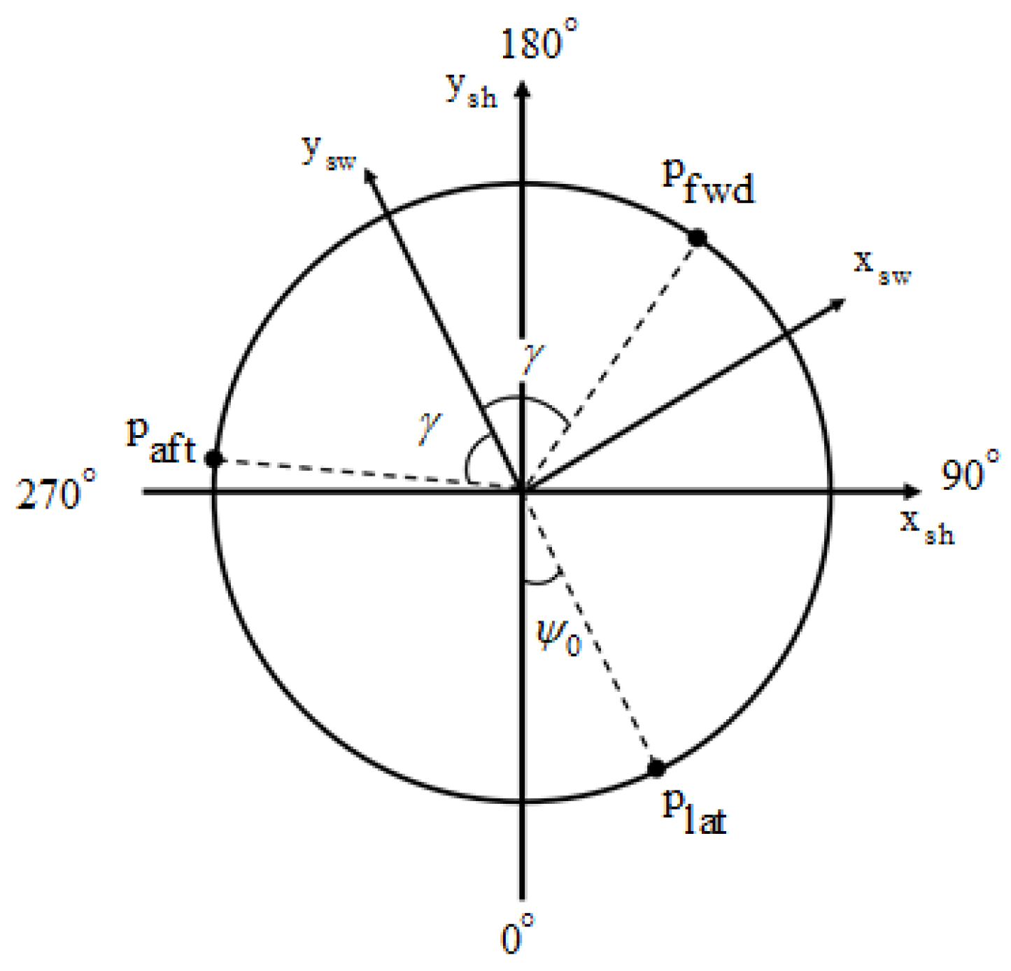
where $\Delta {\theta }_{1s}{}^{\prime }, \Delta {\theta }_0{}^{\prime }$ refers to the actual blade control input after the actuator failure defined in (4)–(9). To be specific, the key parameters of the swashplate [29] are $\gamma =90°, r_{\mathrm{r}}/r_{\mathrm{nr}}=1.17$. Thus, an increase of the longitudinal cyclic pitch $\Delta {\theta }_{1s}{}^{\prime }$ results in:

Case 1 (forward actuator failure): a decrease of the collective pitch of $\Delta {\theta }_0{}^{\prime }=-\Delta {\theta }_{1s}{}^{\prime }/1.17$.

Case 2 (aft actuator failure): an increase of the collective pitch of $\Delta {\theta }_0{}^{\prime }=\Delta {\theta }_{1s}{}^{\prime }/1.17$.

Case 3 (lateral actuator failure): no influence on the collective pitch.

It is shown from the above analysis that, because modern helicopters share similar swashplate structures, although a UH-60 helicopter is taken as a sample model, such method is also applicable for other helicopters, including large-scale helicopters and small-scale helicopters.

The path constraints are chosen as

$$z\ge 0 \mathrm{m},0 \mathrm{m}/\mathrm{s}\le v_x\le 70 \mathrm{m}/\mathrm{s}, v_z\le 10 \mathrm{m}/\mathrm{s}, \left|\theta \right|\le 40°, \left|q\right|\le 40°/\mathrm{s}$$

where descent rate, pitch angle and pitch rate are limited mainly to avoid vortex ring state [21] and fierce maneuvers. The touchdown speed and attitude are limited by terminal constraints, chosen as:

$$\begin{array}{l}0 \mathrm{m}/\mathrm{s}\le v_x(t_f)\le 15 \mathrm{m}/\mathrm{s}, 0 \mathrm{m}/\mathrm{s}\le {\mathrm{v}}_z(t_f)\le 3 \mathrm{m}/\mathrm{s}, \\ -10°\le \theta {(\mathrm{t}}_f)\le 15°, -15°/\mathrm{s}\le q{(\mathrm{t}}_f)\le 15°/\mathrm{s}\end{array}$$

The weight factors of the terminal cost described in Equation (19) are chosen as $W_x=0.7, W_z=1.0$.

Sets of speed sweeps of the three actuator failure cases are conducted under the above optimal control constraints. The speed sweeps range from 5 m/s to 70 m/s. Successful safe landing trajectories of the three actuator failure cases are shown and discussed. To be specific, the trajectories are shown and discussed in two groups. The first group demonstrates the trajectories of the same initial conditions for each actuator failure case. The second group demonstrates typical trajectories with different initial states for each actuator failure case, due to the safe boundaries are different for each failure case, which will be discussed later. Figure 2 compares the three failure cases at the same flight speed of 20 m/s and the same altitude of 50 m.

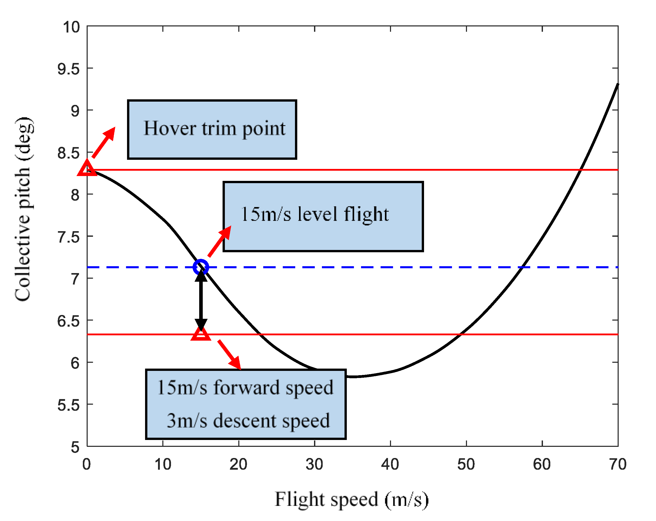
Apparently, when landing, while the vertical speeds are all within the safe landing upper limit of 3 m/s, the resulting forward landing speeds are different. In particular, the forward landing speeds are 12.7 m/s, 8.7 m/s and 0.0 m/s, respectively. The characteristic “bucket profile” of the collective pitch during level flight is shown in Figure 3, which means a steady flight of a lower forward speed near the hover point requires a higher collective pitch. Given the target landing longitudinal velocity of 15 m/s, if the collective pitch before the actuator failure falls in the range of the lower red line and the blue line, there will be a descending rate within 3 m/s at the specific forward speed.

Meanwhile, in order to decelerate, given the same longitudinal cyclic pitch, the collective pitch is decreased for case 1, increased for case 2, and kept constant for case 3. Therefore, the steady forward landing speed of case 1 is highest among the three cases, followed by a lower landing forward speed of case 2, and the lowest landing forward speed of case 3. The above analysis agrees with the trajectory results shown in Figure 2.

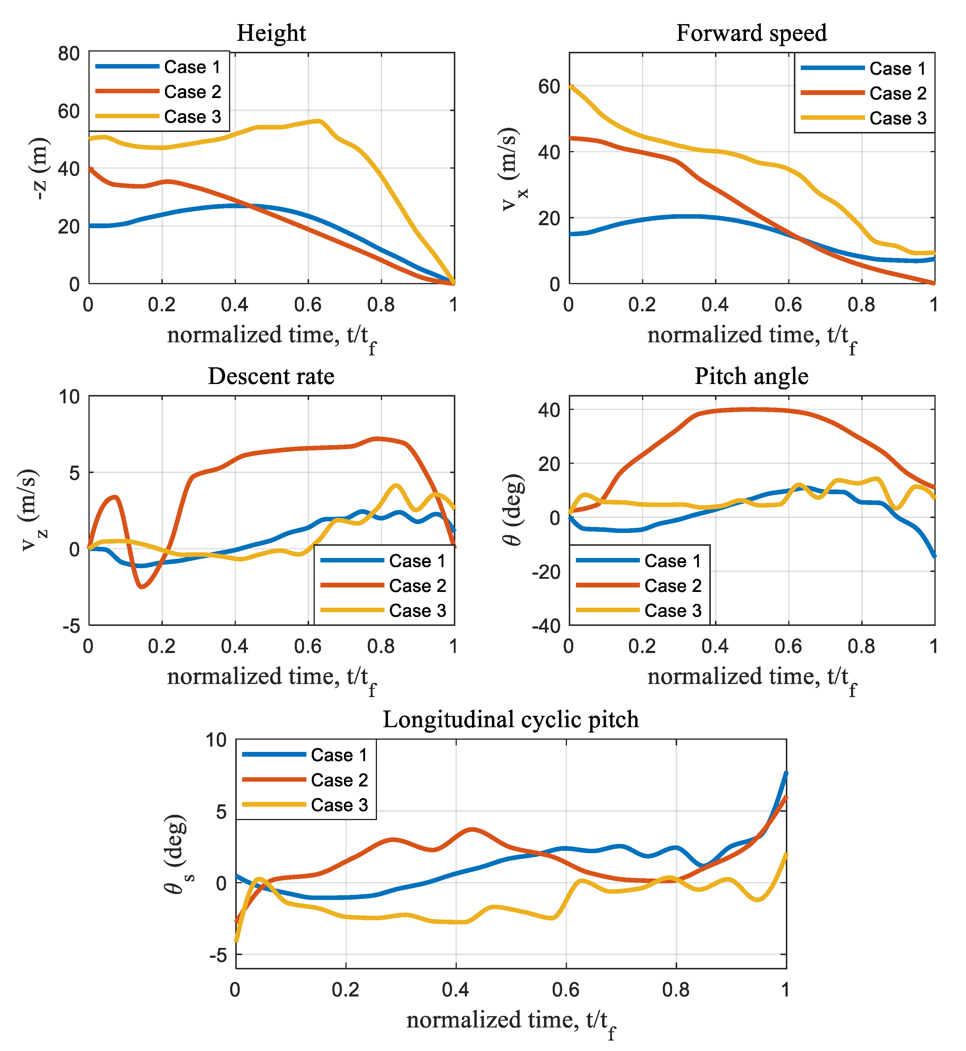
Three typical landing trajectories with different initial forward velocities and altitudes of all actuator failure cases are demonstrated in Figure 4, which are namely 15 m/s for the forward actuator failure in case 1, 44 m/s for the aft actuator failure in case 2 and 60 m/s for the lateral actuator failure in case 3. In case 1, the helicopter encounters the actuator failure at a very low altitude of 20 m. It is then accelerated to gain enough height before deceleration and descent. This shows a significant difference from the autorotation procedure, where the initial altitude is a key factor that determines whether the helicopter can be landed successfully. As for situations of actuator failures, the altitude can be adjusted by a slight adjustment of the longitudinal cyclic pitch. In case 3, the longitudinal cyclic pitch is carefully handled, and the helicopter goes through a procedure consisting of both ascending and descending. The helicopter eventually decreases to a safe velocity when it touches down. The maximum safe initial forward speed, which the algorithm can obtain after the aft actuator failure (case 2), is also demonstrated in Figure 4, represented by the red line.

Other safe boundaries of all the actuator failure cases are obtained by sweeps of speed from 5 m/s to 70 m/s. The results can be described as:

Safe zone for case 1: $v_x\in \left[5 \mathrm{m}/\mathrm{s}, 21 \mathrm{m}/\mathrm{s}\right]$

Safe zone for case 2: $v_x\in \left[14 \mathrm{m}/\mathrm{s}, 44 \mathrm{m}/\mathrm{s}\right]$

Safe zone for case 3: $v_x\in \left[5 \mathrm{m}/\mathrm{s}, 25 \mathrm{m}/\mathrm{s}\right]\cup \left[56 \mathrm{m}/\mathrm{s}, 65 \mathrm{m}/\mathrm{s}\right]$

The safe zones are reasonably different for different actuator failure cases. For the lateral actuator failure (case 3), the collective pitch is not affected by longitudinal manipulations. Thus, within the speed range of 25 m/s to 56 m/s, the position of the collective pitch is too low to sustain a low-speed flight. For the forward actuator failure (case 1), the deceleration from high speed leads to a considerable reduction in the collective pitch. Thus the safe zone is smaller compared to case 1. It is similar for the aft actuator failure (case 2); however, with an increase in collective pitch when decelerating, the safe zone has a wider low-speed boundary compared with case 1. Note that the boundaries of the safe forward speed closely depend on the safe landing requirements. Moreover, if the helicopter cannot touch down with wheel gears, which means a much smaller limitation of forward landing speed is required, there will be a significant reduction in the range of the above safe zones. Another difference lies in the specific control geometry of the helicopter. As shown in Section 2, the radius ratio and the distribution angle $\gamma$ determine the influence on the collective pitch by the other two cyclic controls. Although due to the requirements of compactness of modern helicopters, the radius of the rotating ring and the non-rotating ring are similar, the above parameters should be determined accordingly.

6. Conclusions

This paper focuses on helicopter safe landing trajectories after swashplate actuator stuck failure occurs in level flights by using the remaining manipulations without introducing other control inputs. The general geometry of a single main rotor helicopter swashplate actuator is analyzed, and new configurations of the control mixer are designed for each actuator failure case, without changing the original geometries of the mechanical structure. With new configurations of the control mixer, the trajectories are obtained with a modified two-dimensional nonlinear helicopter dynamic model by the optimal control method. Although the vertical channel is given up due to swashplate actuator failure, results show that the helicopter is still able to land successfully by proper longitudinal manipulations. Results of the trajectories with various initial conditions for each actuator failure case are shown. The results agree with the characteristic “bucket profile” of the collective pitch in level flight. The velocity boundaries of the optimal control problem are found by speed sweeps, which show the safe zones are different with different actuator failure cases. In particular, via the optimal control method proposed in this study, larger safe zones are found for the lateral and aft actuator failure cases, and a tighter zone is found for the forward actuator failure case. Further potential improvements will be introducing a high fidelity helicopter dynamic model, which could be: (1) employing a six-degree-of-freedom helicopter model; (2) introducing more state variables of the rotor induced velocity.