Article

Development of Equipment and Application of Machine Learning Techniques Using Frequency Response Data for Cap Damage Detection of Porcelain Insulators

1
KEPCO Research Institute, Daejeon 34056, Korea
2
Department of Electrical and Computer Engineering, Sungkyunkwan University, Suwon 16419, Korea
3
Department of Safety Engineering, Incheon National University, Incheon 22012, Korea
4
Research Institute for Engineering and Technology, Incheon National University, Incheon 22012, Korea
*
Authors to whom correspondence should be addressed.
Appl. Sci. 2020, 10(8), 2820; https://doi.org/10.3390/app10082820
Submission received: 30 March 2020 / Revised: 14 April 2020 / Accepted: 16 April 2020 / Published: 19 April 2020
(This article belongs to the Section Applied Industrial Technologies)

Abstract

:
The most common method for inspection of insulators is to measure the change of electrical characteristics such as electric resistance and partial discharge. However, even if there is no physical damage, these values vary depending on the temperature, humidity, and chloride content of the atmosphere. In this respect, an alternative to such methods can be the impact response test, and a frequency response function (FRF) obtained from the test has been widely used as a tool for damage detection. In this study the FRF was applied to identify the cap damage of porcelain insulators. In addition, to solve the danger of high voltage and poor field accessibility near the insulator, a device with high field applicability was developed to measure FRF from a long distance using an auto impact hammer and Micro Electro Mechanical Systems (MEMS) technology. Even though the FRF is most suitable for inspection of porcelain insulators, dynamic characteristics such as natural frequencies may vary depending on manufacturing errors, installation conditions, etc., which may cause difficulties in damage identification. To overcome this limitation, the machine learning (ML) method was applied in this study to provide a diagnostic method that ensured consistent and accurate judgment. As a result of predicting the normal and the cap damage data using the support vector machine (SVM), bagging, k-nearest neighbor (kNN), and discriminant analysis (DA) methods, the overall F1 score was over 87% and the bagging method achieved the highest accuracy. In this study, the frequency range and dynamic characteristics that are sensitive to the physical damage of the insulator were derived and, based on this, the optimum ML methods with improved equipment could provide analysis with higher accuracy and consistency than general analysis using the FRF.

1. Introduction

Electricity demand is increasing rapidly owing to modern industrial development, mechanical system automation, global warming, and increasing demand for electric vehicles. To reliably supply such a large amount of power, high transmission voltage is required, and thus, a transmission line with high insulation is required. The insulator mechanically fixes the transmission line to the transmission tower and plays an important role in determining the reliability and safety of the transmission line, such as securing an insulation gap between the transmission line and the transmission tower through electrical insulation [1,2]. In Korea, a significant amount of effort has been invested since the beginning of the 21st century to apply polymer insulators that are easy to manufacture and install, have excellent durability and pollution resistance, and are light and easy to manufacture [3,4]. However, owing to frequent accidents caused by their breakage, porcelain insulators are mostly used in transmission lines of 154 kV or more. In Korea, more than 99% of porcelain insulators are used in transmission lines, and of the 9.8 million porcelain insulators installed, 5.1 million are NGK insulators, Ltd. produced in Japan, accounting for 52% of the total. Among these, more than 1.2 million porcelain insulators installed have 154 kV transmission lines, and approximately 0.8 million insulators have been used for more than 30 years. Insulators do not suffer immediate deterioration or mechanical damage when they are used for longer than their useful life [5].
However, stress accumulation and deterioration of porcelain insulators may cause a sudden breakdown of the insulator due to exposure to an environment of continual stress. This can lead to accidents in which the power line breaks or falls [6]; further, power outages caused by problems with porcelain insulators can be extensive, and can lead to economic and human injury and material damage. To prevent this, it is necessary to develop measuring equipment and inspection technology to allow reliable verification.
Most techniques for detecting damage to an insulator focus on checking the insulation performance of the insulator from an electrical standpoint. Commonly used contact inspection methods in the field include the HI-Pot test, partial discharge measurement method, electric field measurement method, and insulation resistance measurement method [7,8,9,10]. In addition, recently, non-contact infrared scanning and image analysis methods for measuring mechanical damage from a long distance have been studied [11,12]. However, for the above measurement method, even if there is no physical damage, these values vary depending on the temperature, humidity, and chloride content of the atmosphere. In addition, the existing methods cannot be effective in identifying the damage of the insulator due to insensitivity to internal and external physical damage, as presented in Figure 1. In particular, internal cap defects and interfacial damage are difficult to find with visual inspection so a method of overcoming this is necessary.
Therefore, it is difficult to identify mechanical damage around the broken or internal pollution of the cap on the porcelain insulator, as shown in Figure 1. In addition, as the porcelain insulator in the transmission line is coupled with the pins of other porcelain insulators, it is difficult to identify damage visually or using image analysis because a part is covered by the porcelain disc component.
In this study, a frequency response function (FRF) method, which is a simple measurement that is minimally influenced by the surrounding environment and easily detects mechanical damage, is applied to detect the damage on the cap. FRF is one of the methods for confirming the dynamic behavior of an object, and displays dynamic responses such as resonance in the frequency domain for a standardized input. A frequency response analysis (FRA) using an FRF has been widely used to identify mechanical damage for various targets such as civil infrastructure [13], automobiles [14], and electric facilities [15,16,17,18]. However, because the insulator of the transmission line cannot be measured in close proximity, it is necessary to develop equipment with high field applicability for measuring the FRF of string-type porcelain insulators. In equipment development, convenience and weight of the equipment should be considered through the application of the latest technology. In addition, in most studies, energy and frequency of peaks are simply analyzed via fast fourier transform (FFT) and FRF graphs using frequency response data [18]. However, currently installed porcelain insulators were made mostly by hand, so there is a little difference in dimensions and mass, and it is difficult to judge damage only by analyzing the dynamic characteristics of the FRF data. Furthermore, boundary conditions in the field may vary depending on the installation environment. To minimize their effects, it is necessary to apply additional analysis methods to improve the reliability of the analysis. Additional analysis methods exist for extracting various features from the FRF to increase the reliability and diversity of the analysis, rather than the peak analysis of the FRF waveform. In this case, a number of quantitative values, such as area, moment, etc., that can be considered in the FRF waveform can be extracted. Moreover, because a large data set can be constructed according to the extracted features, it is necessary to apply a method for reducing the data size and maintaining the primary characteristics. Neighborhood component analysis (NCA), a major dimension reduction method, is applied to test multiple objects or to identify biases of numerous results from different locations. NCA has been found to be effective in reducing dimensions by identifying trends according to which large amounts of data are contained [19]. NCA is a method for finding feature spaces such that the probabilistic nearest neighbor algorithm provides the best accuracy. In this study, NCA was employed to find the space of features and visualize the division by reflecting the class of porcelain insulators that was known.
In addition, to improve the reliability of the analysis, the machine learning (ML) method was applied to provide a diagnostic method that ensured consistent and accurate judgment. For example, the support vector machine (SVM), one of the most widely used supervisory algorithms for binary classification, employs kernel functions, such as linear, polynomial, and radial functions, to distinguish objects belonging to different classes [20,21]. One of the ensemble classification methods, the bagging method, is another name for bootstrap aggregation. It is generally classified based on a decision tree, and it is a method for changing the number of boosts to improve classification accuracy [22,23]. The k-nearest neighbor (kNN) method is a nonparametric method that was used in statistical applications in the early 1970s. It finds the k sample group closest to an unknown sample in the data set, and is a method for finding the optimal classification value by changing the response variable k, which plays an important role in classifier performance [24]. Discriminant analysis (DA) is a method for classifying data by making decision boundaries through learning about data distribution. The goal is to project the data onto a particular axis and to find a straight line that can distinguish both classes [25]. As such, various ML methods are widely used for cancer prediction in medical fields, determination of normal states and abnormalities in civil structures, and classification of cracks in mechanical fields. This classification method can be used to improve the reliability of the analysis and the ease of judgment.
In this study, ML methods using four classification models, namely, SVM, ensemble, kNN, and DA, were used for damage assessment of the cap of porcelain insulators used in 154 kV transmission lines. In addition, 88 samples were collected from transmission towers subject to various environmental conditions in different regions to increase the reliability of the analysis. Based on the improved equipment, a ML model that ensured consistent and accurate judgement was developed that employed MATLAB software to distinguish the distribution area of normal and cap damage data.

2. Materials and Methods

2.1. Types of Insulators

In this study, porcelain insulator specimens manufactured by the NGK company of Japan were used. The number of test specimens used based on materials and conditions is listed in Table 1. The number of normal cristobalite samples is 59, where 3 exhibit cap damage and 1 exhibits artificial internal damage. The number of normal alumina samples is 22. A specimen exhibiting artificial internal damage is one on which an artificial pollution (AP) test was performed using brine [26]. In the case of cap damage that can occur on transmission lines, the breakage of the cap, which occurs suddenly due to accumulation of fatigue under constant tensile load, has been described. In addition, internal damage was considered due to the contamination of ceramic insulators used on the shore, although there was no external damage.

2.2. Frequency Response Function (FRF)

The porcelain insulator is manufactured by NGK Ltd., so it is difficult to confirm the exact physical properties of the various types of cement used therein. It is also difficult to calculate the theoretical frequency response function (FRF) because the manufacture of porcelain parts involves manual labor. Therefore, the FRF was calculated using Equation (1) and the data measured from the experiment conducted on the developed equipment [27]. In Equation (1), the FRF is expressed as H(f), and the relationship between X(f), the power spectral density of the time signal measured by an auto impact hammer, and Y(f), the power spectral density of the time signal measured by a Micro Electro Mechanical Systems (MEMS) sensor, is given:
F R F = H ( f ) = Y ( f ) X ( f )

3. Developed Equipment and Experimental Setup

3.1. Schematic of Developed Equipment

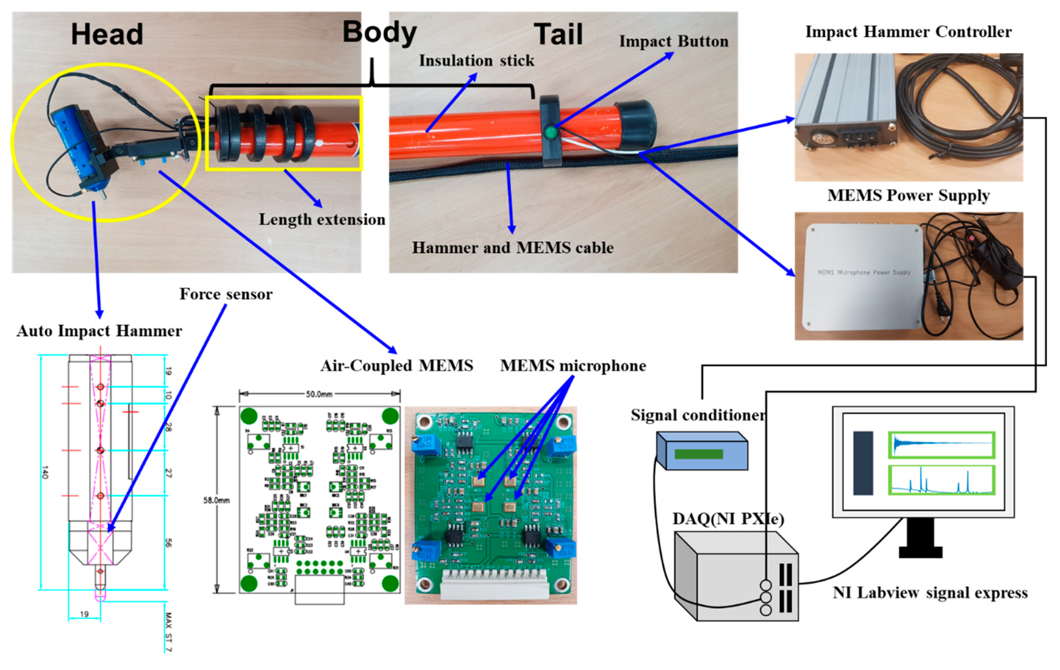
Commonly employed FRF tests are performed by attaching an accelerometer to the structure and striking the measurer with an impact hammer by the user. However, due to the inaccessibility of the porcelain insulator owing to the field conditions in which high voltages pass, it is necessary to develop suitable equipment that can measure over long-distance ranges according to basic operating principles. The device developed in this study is shown in Figure 2. The developed device is divided into three parts: the head, including the auto impact hammer and signal receiver; the body, made to extend the length of the insulating material; and the tail, consisting of the impact button and handle. It also includes a controller that can adjust the impact strength of the auto impact hammer and a device for power supply. The auto impact hammer (330AE-05) in the head region, manufactured by AISYSTEMS Ltd. in Korea, can control the impact strength up to 100 N, and includes a force sensor to measure the input energy during striking. The MEMS microphone (Zero-Height SiSonicTM Microphone) was manufactured by KNOWLES Ltd. in USA, and reduces weight for user convenience in the signal receiver. The contactless MEMS microphone was used in consideration of field situations where direct contact is difficult [28]. Four sensors are used to reduce data measurement errors and ensure data reliability, and the frequency range of the sensors is 0 to 80 kHz. The insulation stick of the body part is made to extend up to 5 m.
The signal conditioner (PCB 482C16) and DAQ (NI PXIe-6366) were used in the developed device for data acquisition. The measurement program used NI Labview signal express to store data at a sampling rate of 500 kS/s, which was analyzed using the MATLAB signal process toolbox, because the stored data are values in the time domain.

3.2. FRF Test Using Developed Equipment

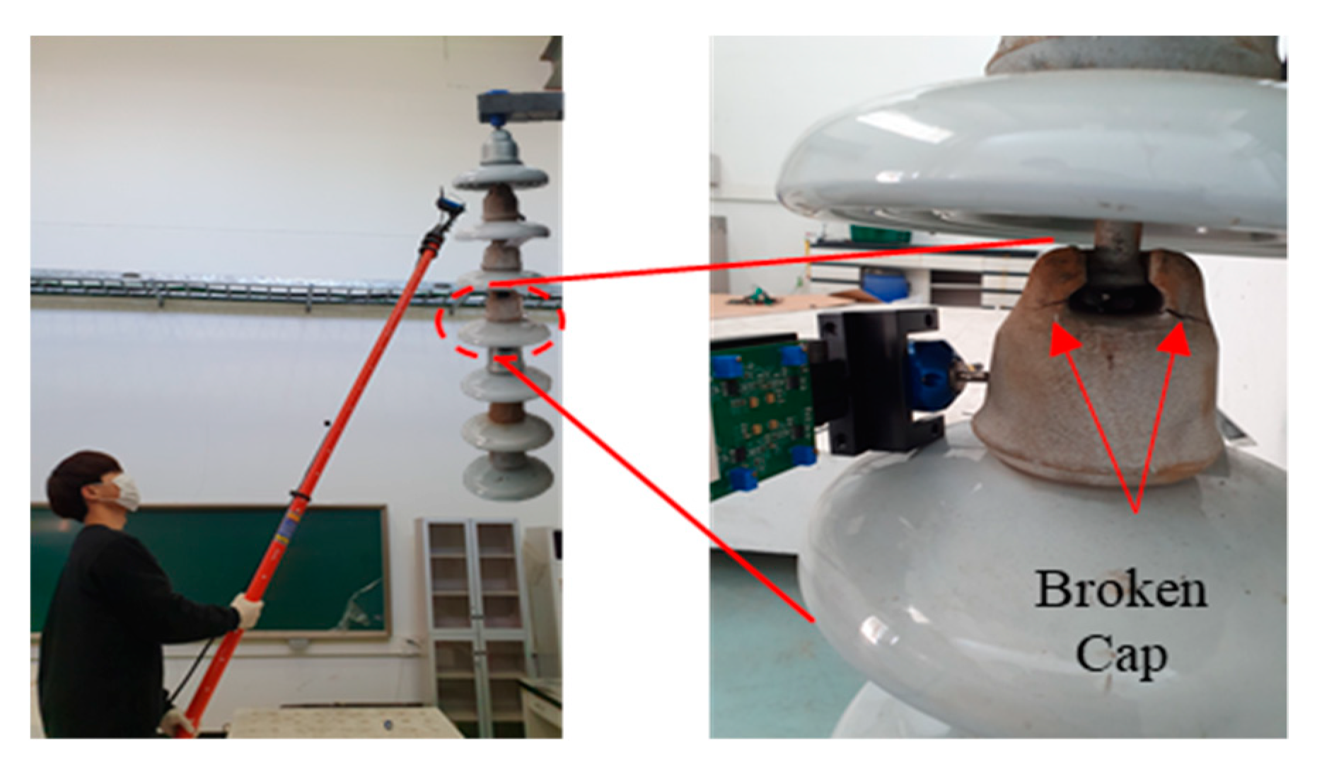
Using the developed equipment, the FRF of the porcelain insulator was measured under the conditions as shown in Figure 3. The left side of Figure 3 shows a string structure in which porcelain insulators are connected in series; first, a method of striking the porcelain was applied to check for damage to the cap.

3.2.1. FRF Results of Porcelain Impact

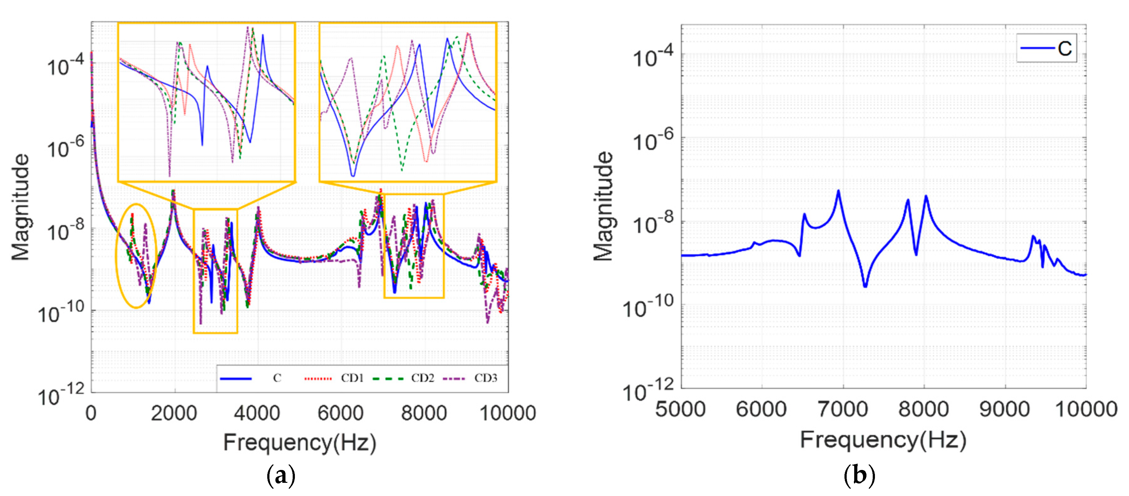
First, analysis was carried out to determine whether the normal and damaged caps were distinguishable for the cristobalite material. The FRF of the normal specimen (C) produced four eigenmodes from 0 to 5 kHz and four eigenmodes from 5 to 10 kHz, as shown in Figure 4a,b. Similar waveforms appeared in other normal specimens, and it was confirmed that no peak other than those of the eight eigenmodes occurred. In the case of cap damage specimens (CD1 to CD3), a new eigenmode was generated below 2 kHz, and the second eigenmode was characterized by low frequency shift. However, the FRF waveform was mostly normal. Differences between the normal and damaged cap specimens have typically been identified by striking porcelain samples, but these minor changes can be difficult to replicate due to the characteristics of porcelain insulators in various manufacturing conditions, and the errors in field experiments. Therefore, the analysis was conducted by striking the cap to derive a clear difference between the normal condition and cap failure.

3.2.2. FRF Results of Cap Impact

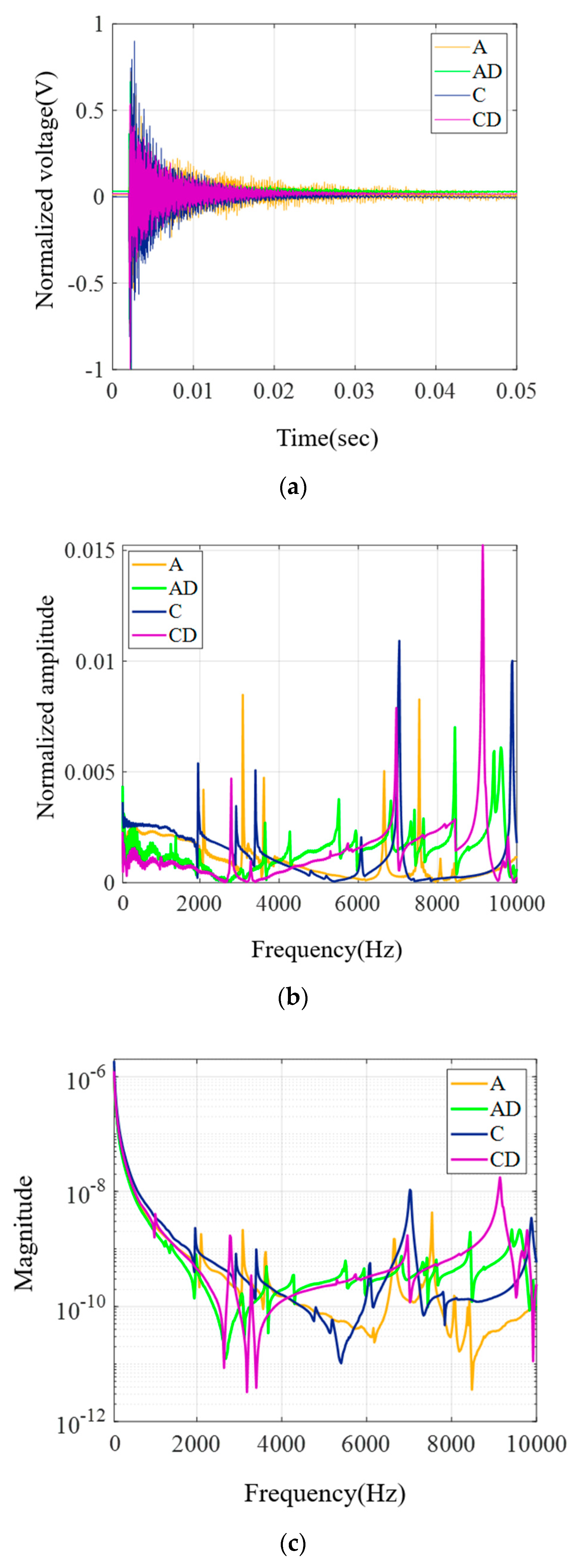
In Figure 4, only the FRF was analyzed via striking of porcelain. However, in Figure 5, the striking of the cap was performed in an attempt to identify the difference between normal and defect caps in (a) time domain, (b) FFT domain, and (c) FRF domain, where A is normal alumina material, C is normal cristobalite material, and AD and CD are metal damage test pieces of each material. In the time domain, the y-axis is normalized to the maximum negative peak; it is difficult to distinguish the difference between the normal and the damaged cap except for the fine envelope difference of the time signal. In the FFT domain, a shift in frequency peaks between the normal and the metal damage specimens was confirmed. However, because the manufacturing of porcelain insulators is different, determining the defects only by the frequency shift of FFT may not be a reliable approach. The eigenmode peak difference was observed in the FRF domain, and it was confirmed that the FRF waveform of the damaged specimen was higher than that of the normal specimen in the frequency range of 4–10 kHz, and the magnitude was higher. Analysis of the data in the FRF domain via investigation of the three domains seems to be a suitable method for more accurately identifying differences.
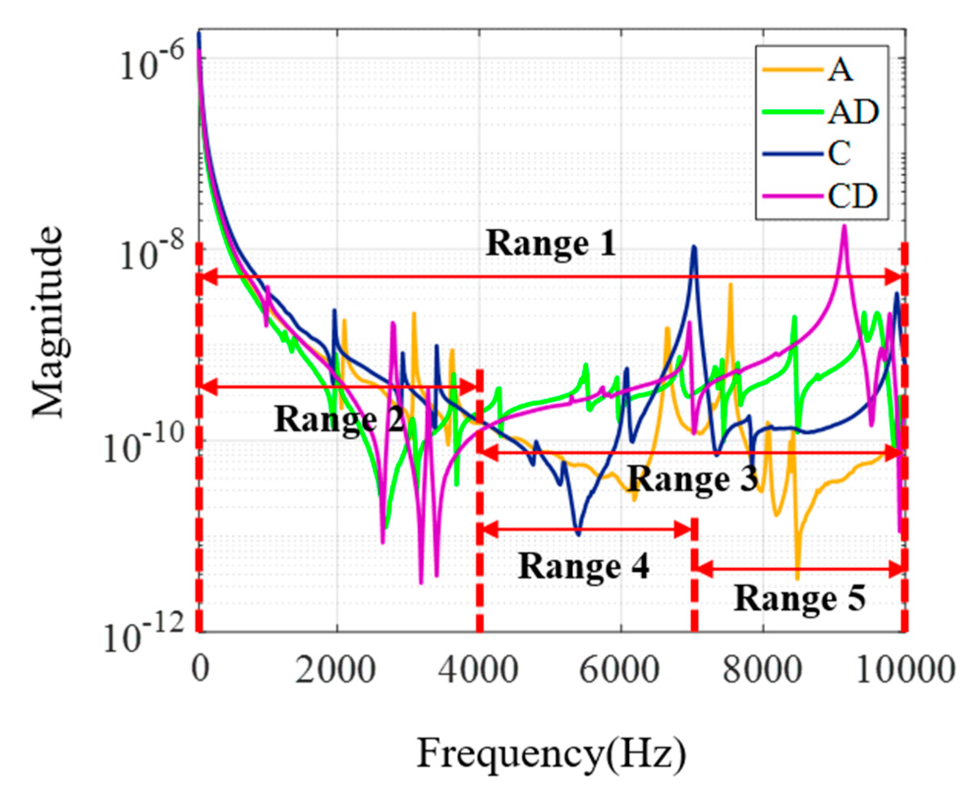
As per the FRF results shown in Figure 5, analyzing all the data obtained from 0 to 10 kHz may prove to be an inefficient method for extracting the correct features. Therefore, for efficient analysis, as shown in Figure 6, the frequency range of the FRF graph is divided into five ranges: 0–10 kHz, 0–4 kHz, 4–10 kHz, 4–7 kHz, and 7–10 kHz. Using these divisions, feature extraction was performed to find the optimal frequency range that distinguishes the normal condition from the defect.

3.3. Procedure of Feature Extraction

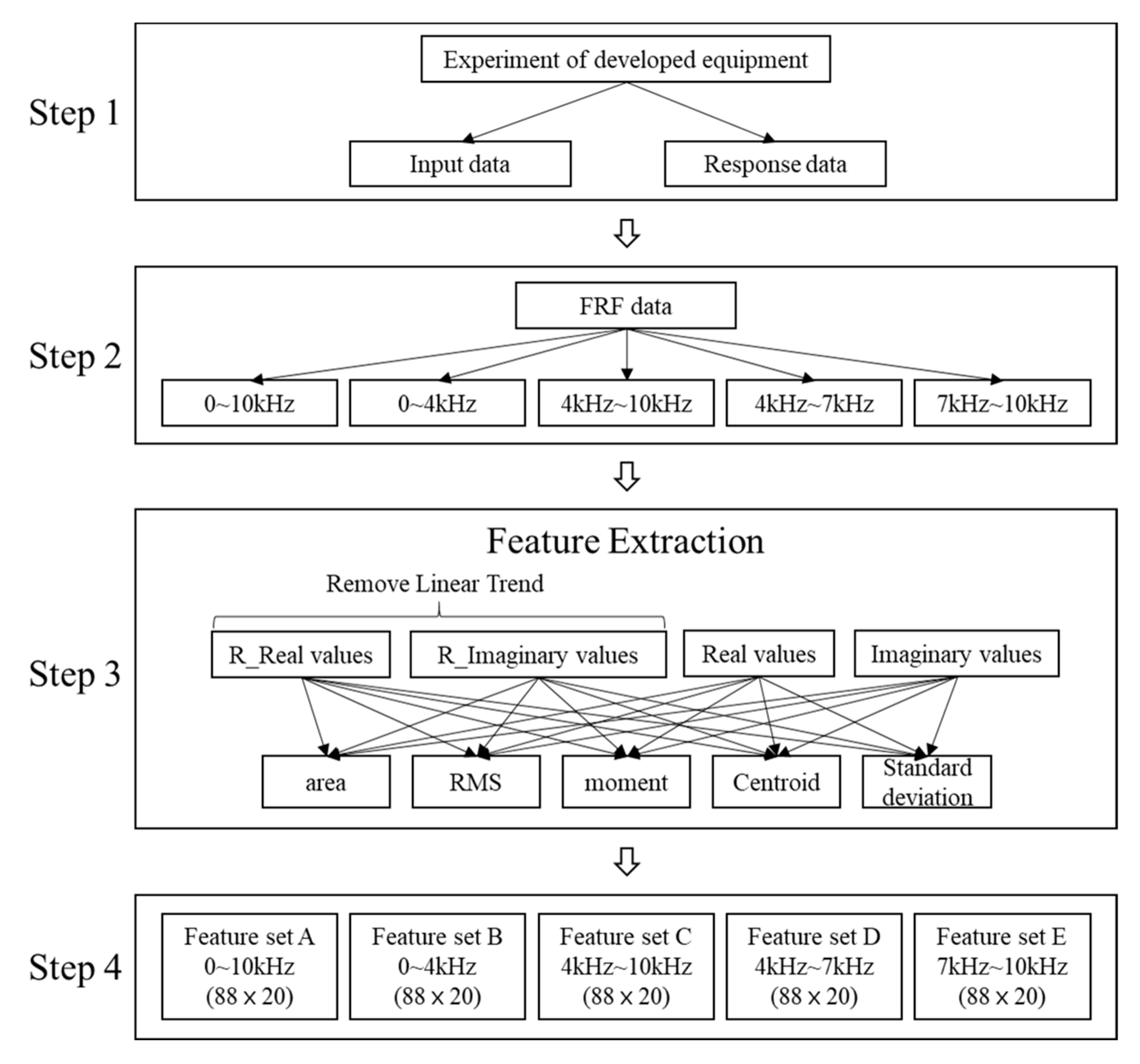
Feature extraction proceeded from step 1 to step 4 as shown in Figure 7. First, in step 1, the FRFs were tested for all porcelain insulators using the developed equipment of Figure 3, and input data and response data were collected. The input data is a signal collected from the auto impact hammer, and output data is a signal collected by the MEMS microphone. In step 2, the input data and response data were converted into the frequency domain by FFT, and the FRF data of each porcelain insulator were calculated using Equation (1). Then, each set of FRF data was extracted separately according to the five frequency ranges identified in Figure 6. In step 3, a total of four basic data sets were constructed, including the real and imaginary values of the FRF data and the data not exhibiting a linear trend between the two values. The original data of the FRF waveform has real and imaginary values, which means that a total of four basic data sets for one FRF waveform are constructed. Next, 20 characteristics were derived by calculating area, root mean square (RMS), cross-sectional primary moment, center, and standard deviation using the four basic data sets [29]. Removal of trends implies subtracting the mean or the best fit line from the data (meaning the least squares). Removing the trends from the data allows us to focus our analysis on variations in the data for the trends. Linear trends generally indicate a systematic increase or decrease in data. Trends are meaningful, but removing trends provides better insights in some analysis types. Whether it is appropriate to remove trend effects from the data often depends on the analytical goal. Finally, in step 4, the data calculated according to the frequency range is divided into feature sets A to E and then used as basic data for NCA analysis.

4. Machine Learning Methods

4.1. Neighborhood Component Analysis (NCA)

NCA is a supervised learning method for classifying multivariate data into separate classes based on a given distance metric for the data. Functionally, it serves the same purpose as the kNN algorithm and directly employs a related concept called the stochastic proximity neighbor [19]. Neighbor factor analysis aims to learn the distance metric by finding a linear transformation of the input data to maximize the average LOO (leave-one-out) classification performance in the transformed space [30]. The key to the algorithm is that the matrix B corresponding to the transformation defines a differentiable objective function for B, and then finds it using an iterative solver such as the conjugate slope drop. One advantage of this algorithm is that the number of k classes can be determined up to a scalar constant as a function of B. Therefore, the use of this algorithm solves the model selection problem. In order to define B, a specific function that describes the classification accuracy of the converted space is defined, and is analyzed by determining the value of B * to maximize this function as shown in Equation (2):
B * = a r g m a x B f ( B )

4.2. Support Vector Machine (SVM)

SVMs consist of hyperplanes or sets of hyperplanes that can be used for classification or regression analysis in one type of ML. SVMs are mainly used for binary classification; there are also linear classifications using hyperplanes and nonlinear classifications employing high-dimensional projection using kernel functions. In general, given a set of data belonging to either class, the SVM creates a non-probability binary classification model that determines which class the new data belongs to, based on the given data set. The classification model is represented as a boundary in the space wherein data is mapped. The SVM algorithm finds the boundary with the largest margin among them [20,31]. The hyperplane can be expressed as a set of points, x, satisfying Equation (3). When data can be linearly separated according to two class sets with a value of 1 or −1, w is the normal vector of the hyperplane, ∙ is the inner product, and b is the deflection constant that fixes the hyperplane at an offset in p-dimensional space.
w · x b = 0

4.3. Bagging

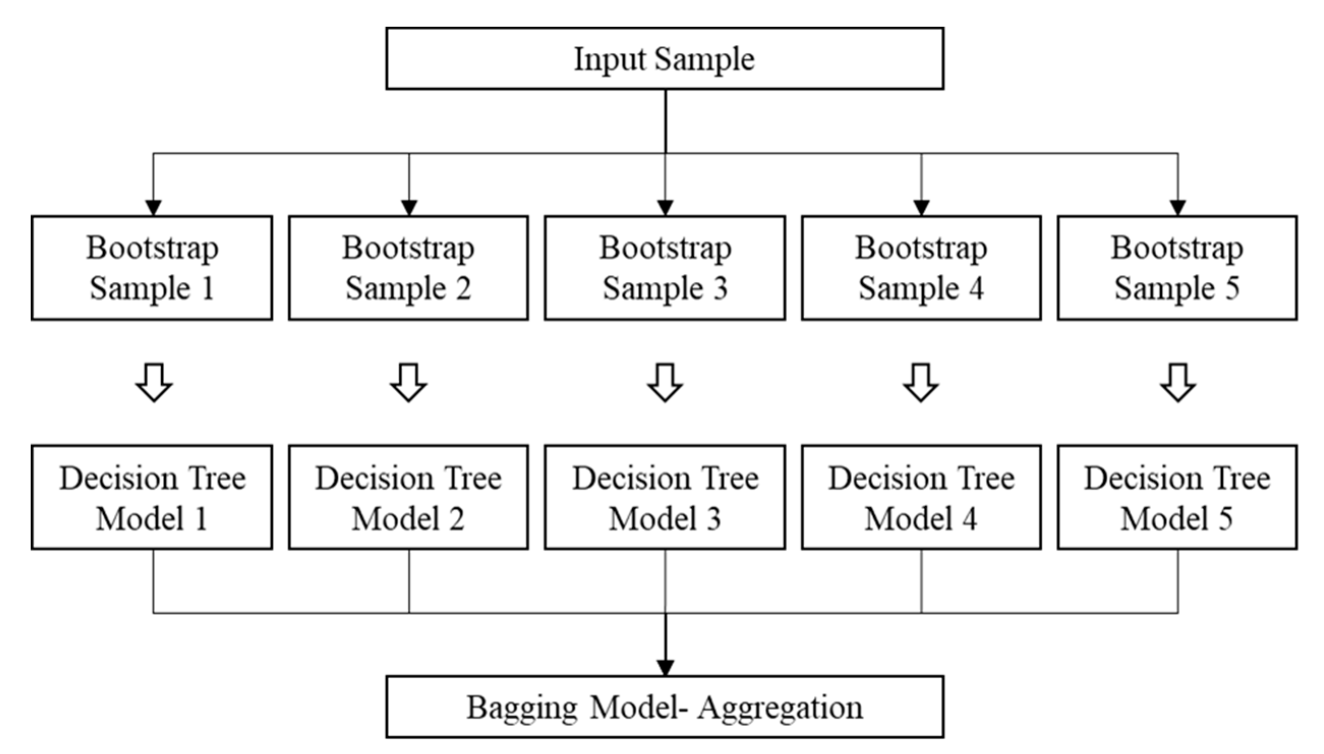
Bagging, also called bootstrap aggregating, is an ensemble method. It is a meta-algorithm used to improve the stability and accuracy of the ML algorithms employed in classification and regression. It also helps to reduce variance and avoid overfitting, and is generally applied to decision tree methods but can be used with any type of method. The bagging method proceeds according to the procedure depicted in Figure 8 [22,23]. In general, in case of categorical data, the predictor is counted by voting, and in case of continuous data, it is counted by the average. In this study, voting was used because the data is categorical.

4.4. k-Nearest Neighbor (kNN)

k-Nearest Neighbor (kNN) is a non-parametric statistics algorithm used in statistical applications. It is a type of supervised learning [24] and is a classification algorithm that classifies data with classes. As the name of the algorithm suggests, it is a method that performs classification by referring to k classes of other data closest to the data in consideration. The distance is measured using the Euclidean distance method shown in Equation (4):
D ( x , y ) = i = 0 n ( x i y i ) 2
where D(x,y) represents the distance between the two selected input vectors, and xi and yi represent the data points. In the classifier, k is a tuning parameter that plays an important role in the performance of kNN [32].

4.5. Discriminant Analysis (DA)

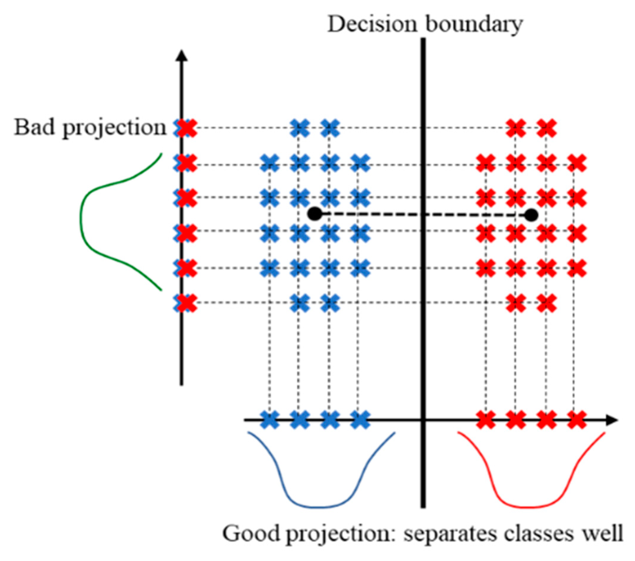
Discriminant analysis (DA) is a data classification method that finds the decision boundary assuming that different classes generate data based on different Gaussian distributions, as shown in Figure 9 [25]. To train the classifier, the fitting function estimates the parameters of the Gaussian distribution for each class, and the trained classifier finds the class with the lowest false classification for predicting a new class of data. When the variable x is projected on a vector (axis) called w and the center (average) vector of each category is m1, m2, the method finds the vector w where m1 and m2 are located far apart. Here, the goal is to maximize the center of both categories and minimize the variance. There are two types of DA, namely, linear discriminant analysis (LDA) and quadratic discriminant analysis (QDA).

5. Analysis and Result

5.1. Feature Extraction Using NCA

For the feature sets A to E, three NCA analyzes were conducted with different functions to identify the most significant features among the 20 data features extracted in Figure 7. NCA was performed using MATLAB, and three functions were used: lgfgs, Minibatch-lbfgs, and sgd. lbfgs is the limited memory Broyden–Fletcher–Goldfarb–Shanno (LBFGS) algorithm, and sgd is the stochastic gradient descent (SGD) algorithm, and minibatch-lbfgs is the stochastic gradient descent with LBFGS algorithm applied to mini-batches. Figure 10 shows three NCA results for feature set A. The feature index in Figure 10 is the order of the features extracted in step 3 of Figure 7, and a large feature weight means that the bias of the data is large. As a result of the analysis, it is confirmed that the 4th, 9th, 14th, and 19th features exhibit the highest bias. These four features are the geometrical moment of area of R real values, R imaginary values, real values, and imaginary values. In other feature sets, the geometrical moment of area showed the greatest bias equally. Therefore, the analysis was performed using features 4 and 9 in each feature set.
Figure 11 shows a 2D plot using two main features (moments of R Real values and real values) derived from NCAs from feature sets A through E. PC1 and PC2 are principal components of the first and second according to feature weight. A and C are normal alumina and cristobalite specimens, respectively, and AD and CD are metal damage test specimens of each material. In addition, the red dashed line can be used to check whether the normal and the damaged caps are linearly separated. As a result of analyzing the graph, data in the ranges of 0–4 kHz, 4–7 kHz, and 7–10 kHz are considered to be inappropriate because some defective data is included in the distribution range of the normal data. In the case of 0–10 kHz data, normal and damaged caps can be linearly distinguished, but the range of overlap of cristobalite and alumina materials is wider than that of the 4–10 kHz range in the distribution of normal data. Therefore, the 4–10 kHz range of the feature set C was set as the frequency region of interest, and the graph of Figure 11c was analyzed. As a result, it was confirmed that the normal and bracket damage data were accurately linearly classified based on the −0.5 value, and the normal cristobalite data and the alumina data were partially intersected but mostly distinguishable. However, the 2D plot results obtained via the NCA can be confirmed immediately, but the same process is required to determine additional data, and it is difficult to accurately determine the nonlinear classification. Therefore, it is necessary to develop a distribution area and a judgment model for material and damage so that an immediate judgment can be made using ML techniques.

5.2. Machine Learning Analysis

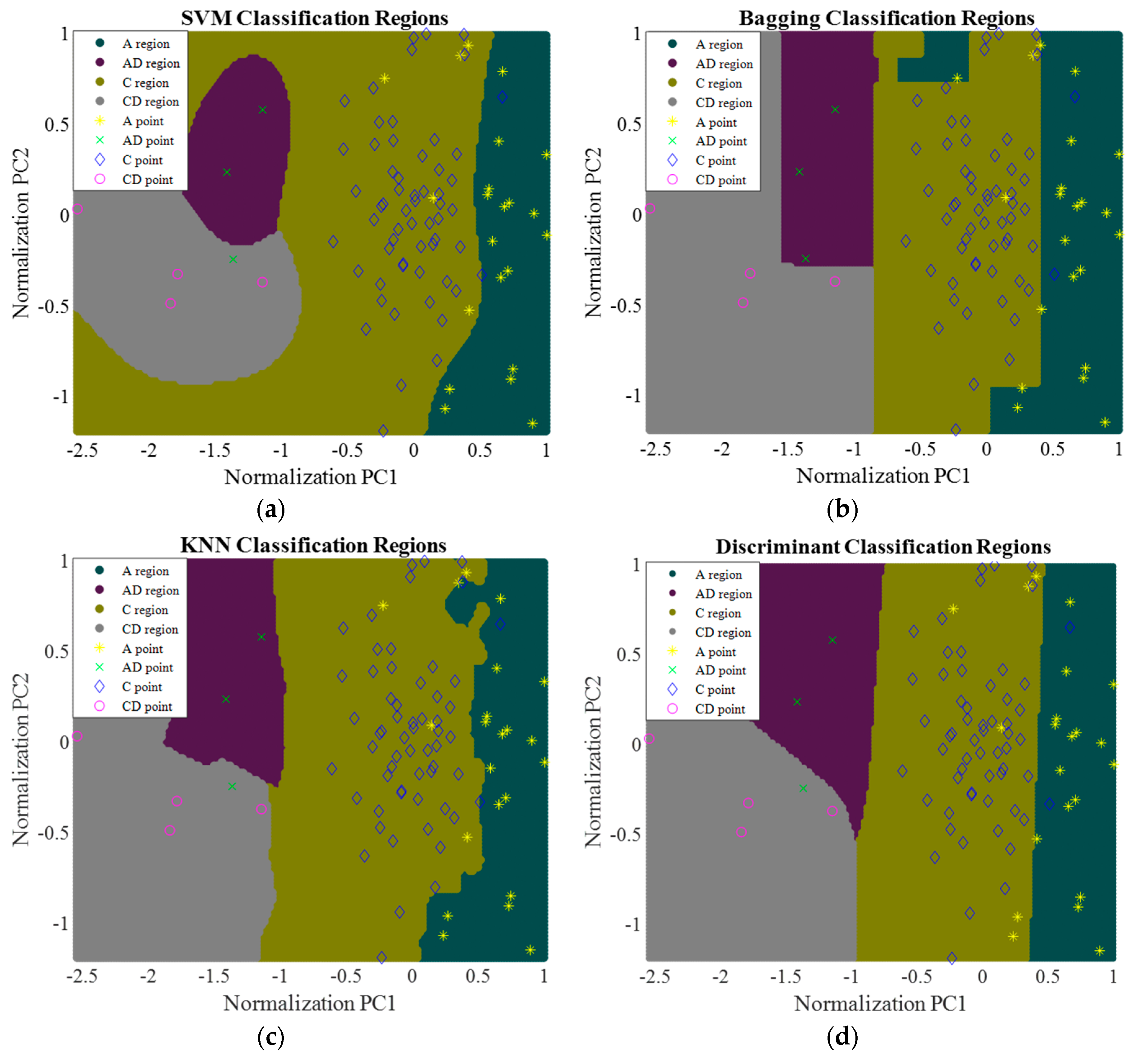
For developing the setting of the post-distribution region and predictive model of the data through ML, the large value in Figure 11c takes a long time, and a problem regarding overload exists, so the analysis was conducted using normalized values. The training sets for the predictive model formation were divided into (class1 and class2), (class1 and class3), (class1 and class4), (class2 and class3), (class2 and class4), and (class3 and class4). Here, class1 and class2 are the normal and the damaged cap data of alumina, and class3 and class4 are the normal and the damaged cap data of cristobalite. Finally, a classification model was merged and formed through six learning phases. The entire data as a test set was evaluated with the developed model. The ML results are shown in Figure 12 and were obtained by estimating the post-distribution area using SVM, bagging, kNN, and DA methods.
In Figure 12a, the SVM performed nonlinear analysis with multi-SVMs using the radial basis function (RBF) as the nonlinear kernel, which is suitable for classification of many classes because the accuracy of the classification is reduced when commonly used linear classifications are employed. Multi-SVM performed analysis by creating a separate classification model for four classes and merging them.
In Figure 12b, the bagging method is used as one of the ensemble methods. It uses several weak learners to extract bootstrap samples several times to train each model and aggregate the learning results. Three bootstraps were used in this study. The bagging method increases the accuracy of class classification by increasing the number of bootstraps, but because it randomly selects bootstrap samples, the range of one class can be separated rather than appear continuously, if data present inside are selected. Therefore, a small number of bootstraps was used.
In Figure 12c, the kNN method creates a template for the search of the nearest neighbors and standardizes and analyzes the predictors. In order to consider the continuity of the class region, the nearest neighbors are designated as one of three types to classify the entire class.
In Figure 12d, the DA method was developed using regularized quadratic discriminant analysis to find the class with the lowest false classification cost, if different classes generate data based on different Gaussian distributions. A more accurate second-order discriminant analysis method was used for multiclass classification.
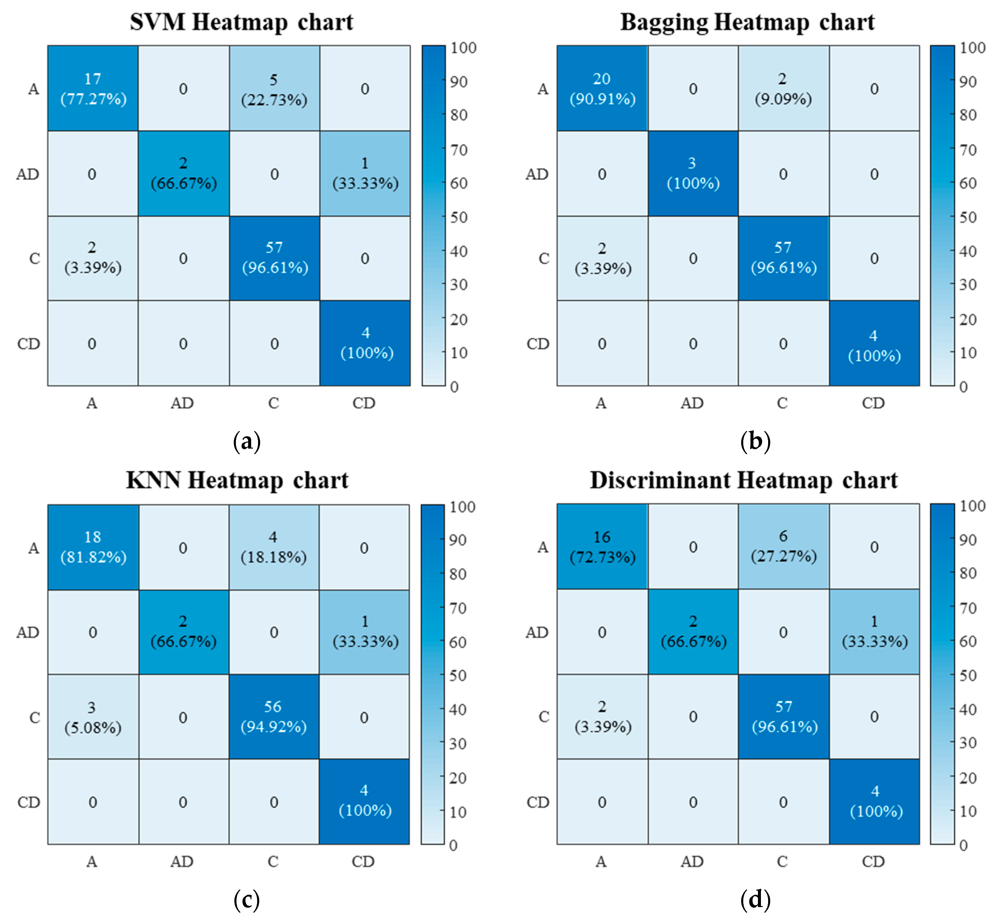
Because a series of processes was carried out, including feature extraction and setting up of frequencies of FRF interest, and eliciting features with significant contributions by NCA, it was possible to clearly distinguish between the normal and damaged cap conditions. Through this, via analysis using four ML methods, a model was developed that distinguishes 100% of normal and gold tool damage data. In addition, the predicted accuracy of the four classes was analyzed using the developed model, and is shown in Figure 13 as a heatmap chart for comparison. As a result of heatmap chart analysis, the classification accuracy of the normal data was similar for the four classification methods, but the bagging method showed the highest accuracy in classification of the damaged cap data. For this reason, for the SVM, KNN, and DA methods, the boundary was separated by the correlation of the two classed for the damaged cap class, so one alumina data with cap damage was determined to be cristobalite. However, in the case of the bagging method, the boundary is divided by using only alumina damage data itself. Therefore, it is judged that the bagging method establishes the most accurate area in the analysis using the data of this study.
In the model development using ML, the accuracy analysis and the F1 score analysis were finally performed for the prediction result of the developed model. In general, the ratio between normal and defect data is similar, and when analyzing two classes, the performance of the model is evaluated using accuracy in the confusion matrix. However, the sample data in this study has significantly less defect data than normal data, and has four classes. Therefore, because it was difficult to accurately evaluate the reliability of the model on the basis of only accuracy, the F1 score was also analyzed. The results of the reliability evaluation and performance of the developed model are presented in Table 2. For each class, the true positive (TP) is the correct prediction for the right class, the false positive (FP) is the incorrect prediction for the right class, and the false negative (FN) is the correct prediction for the wrong class. Precision can be calculated using Equation (5) for TP and FP in each class. Recall can be calculated using Equation (6) for TP and FN in each class. Then, the precision and recall average can be obtained using Equations (7) and (8), and the F1 score can be calculated using Equation (9). The F1 Score is the harmonic mean of recall and precision for evaluating the performance of multiple classification models.
P r e c i s i o n = T P / ( T P + F P )
R e c a l l = T P / ( T P + F N )
A v e r a g e   P r e c i s i o n = { P ( A ) + P ( A D ) + P ( C ) + P ( C D ) } / 4
A v e r a g e   R e c a l l = { R ( A ) + R ( A D ) + R ( C ) + R ( C D ) } / 4
F 1   Score = 2 × A v e r a g e   P r e c i s i o n × A v e r a g e   R e c a l l A v e r a g e   P r e c i s i o n + A v e r a g e   R e c a l l
As a result of the analysis of the developed model, the bagging method took about two–three times longer to develop the model than the other three models, and it was determined to be the most reliable model, exhibiting an accuracy of 95.45% and F1 score of 96.88%. The other three models showed similar results in terms of accuracy and F1 score. Because a clear feature was derived at the early stage of feature extraction, a model suitable for classifying normal caps and defects was developed.
However, additional analysis was conducted against data overfitting. For SVM, ensemble, kNN, and DA models, the five-fold cross validation and error were analyzed using ‘crossval’ and ‘kfoldLoss’ functions in MATLAB. Accuracy of the ensemble and kNN models was reduced by up to 2% compared to the F1 score in Table 2, and the accuracy of the SVM and DA models was reduced by up to 1%. The over-fitting problem between normal cristobalite and alumina data was alleviated and data were closer to the generalized model.
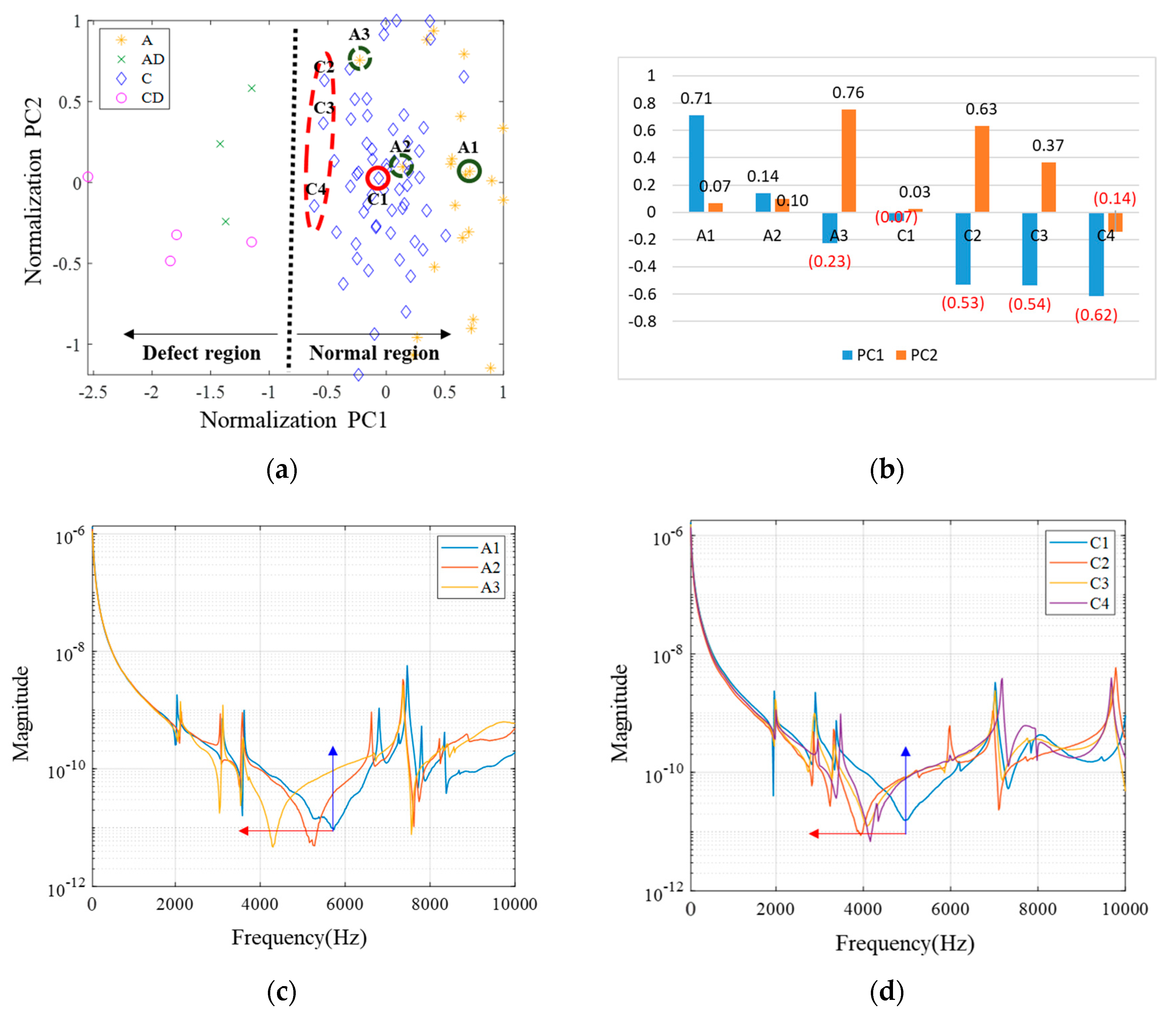
Most of the material classification is performed, but there are some overlapping portions at the interface. This may be an error that occurs because the insulator is fabricated by hand. In addition, there is a material classification in damage, but the FRF waveform due to damage is so variable that it may even be at the interface. Moreover, the data distributed at some interfaces and the data distributed at the center of the normal data are reanalyzed in Figure 14. In Figure 14a, the interface data and unusual values are sampled. The PC1 and PC2 values of the selected A1–3 and C1–4 data are shown in Figure 14b. FRF results for normal and interface data and normal and unusual data are plotted in Figure 14c,d.
In the alumina and cristobalite materials, the FRF results of the samples with normal data and boundary data (C1–C4) or normal data and unusual data (A1–A3) confirmed that the first negative peak shifted to a low frequency, and the FRF waveform was distributed higher than normal. These results are similar to those of the FRF of the defect test specimens. Moreover, because the damage cannot be confirmed in appearance, it may be caused by sudden breakage due to continuous loads during the insulator manufacturing process or as a result of excess voltage conditions; it may be necessary to repair or replace it in these cases.

6. Conclusions

In order to measure porcelain insulators used in transmission towers, equipment with high field applicability was developed utilizing an auto impact hammer and MEMS sensors. The developed equipment was used to measure string porcelain insulators used at 154 kV. Based on the frequency response function, the frequency range of interest was set, feature extraction was performed, and four ML algorithm types were applied to distinguish normal and damaged caps. The damage assessment model was developed by analyzing the correlation between features and materials and defects extracted from the frequency response data using 88 porcelain insulators. Results and conclusions can be summarized as follows:
  • Field adaptable equipment was developed via the use of auto impact hammers and MEMS sensors to improve the convenience of measuring equipment and reduce weight.
  • In the FRF test results, for damage to the cap, direct striking of the cap was more clearly distinguishable between normal and damaged caps than striking the porcelain section. Moreover, the accuracy of material and defect data classification was increased by setting the frequency region of interest from 4 kHz to 10 kHz for the FRF results of the caps.
  • Four classification methods were used to set the post-distribution area of data through ML classification, and a model was developed to distinguish between normal and damaged cap data to an extent of 100%. Further, all models exhibited a high accuracy in classifying the material of normal data, and the bagging method had the best prediction ability in classifying the material of defect data.
  • The distinction between normal and cap damage specimens was correct, but some data were found to exist within the distribution ranges of different classes, depending on the material. The reason for this is that porcelain insulators involve a manual process during manufacture, which may lead to manufacturing errors. Moreover, the FRF of the normal specimen present near the interface between the normal and the damaged area is like the FRF of the damaged cap specimen, and thus management of the porcelain insulator representing these waveforms is necessary. In the future, to develop a better predictive model, it would be necessary to precisely set the distribution area using various cap damage specimens according to the degree of damage.

Author Contributions

I.H.C., J.A.S. and J.B.K. conceived and designed the experiments; Y.G.Y. and T.K.O. performed the experiments and analyzed the data; I.H.C. and J.S.Y. contributed device/analysis tools; Y.G.Y. and T.K.O. wrote the paper. All authors have read and agreed to the published version of the manuscript.

Funding

This research was funded by Korea Electric Power Corporation (KEPCO). This work was supported by Research Assistance Program (2020) in the Incheon National University.

Conflicts of Interest

The authors declare no conflict of interest.

References

  1. Looms, J.S.T. Introduction. In Insulators for High Voltages, 7th ed.; Peter Peregrinus Ltd.: London, UK, 1988; pp. 1–3. [Google Scholar]
  2. Vaillancourt, G.H.; Bellerive, J.P.; St-Jean, M.; Jean, C. New live line tester for porcelain suspension insulators on high-voltage power lines. IEEE Trans. Power Deliv. 1994, 9, 208–219. [Google Scholar] [CrossRef]
  3. Momen, G.; Farzaneh, M. Survey of Micro/Nano Filler Use to Improve Silicone Rubber for Outdoor Insulators. Rev. Adv. Mater. Sci. 2011, 27, 1–13. [Google Scholar]
  4. Karady, G.G.; Shah, M.; Brown, R.L. Flashover mechanism of silicone rubber insulators used for outdoor insulation. IEEE Trans. Power Deliv. 1995, 10, 1965–1971. [Google Scholar] [CrossRef]
  5. Choi, I.H.; Kim, T.K.; Yoon, Y.B.; Kim, T.Y.; Nguyen, H.T.; Yi, J.S. A Study on the Life-Time Assessment Ways and Various Failure Types of 154 kV Porcelain Insulators Installed in South Korea. Trans. Electr. Electron. Mater. 2018, 19, 188–194. [Google Scholar] [CrossRef]
  6. Bardeen, A.W.; Sheadel, J.M. Corrosion as it affects insulator and conductor hardware. In Proceedings of the AIEE Winter General Meeting, New York, NY, USA, 30 January–3 February 1956; pp. 491–501. [Google Scholar]
  7. Cherney, E.A.; Am, D.E. Development and application of a hot-line suspension insulator tester. IEEE Trans. Power Appar. Syst. 1981, PAS-100, 1525–1528. [Google Scholar] [CrossRef]
  8. Padma, V.; Raghavan, V.S. Analysis of insulation degradation in Insulators using Partial Discharge analysis. In Proceedings of the 2011 3rd International Conference on Electronics Computer (ICECT), Kanyakumari, India, 8–10 April 2011; pp. 110–114. [Google Scholar]
  9. Vaillancourt, G.H.; Carignan, S.; Jean, C. Experience with the detection of faulty composite insulators on high-voltage power lines by the electric field measurement method. IEEE Trans. Power Deliv. 1998, 13, 661–666. [Google Scholar] [CrossRef]
  10. Cavallini, A.; Chandrasekar, S.; Montanari, G.C.; Puletti, F. Inferring ceramic insulator pollution by an innovative approach resorting to PD detection. IEEE Trans. Dielectr. Electr. Insul. 2007, 14, 23–29. [Google Scholar] [CrossRef]
  11. Ha, H.; Han, S.; Lee, J. Fault detection on transmission lines using a microphone array and an infrared thermal imaging camera. IEEE Trans. Instrum. Meas. 2012, 61, 267–275. [Google Scholar] [CrossRef]
  12. Miao, X.R.; Liu, X.Y.; Chen, J.; Zhuang, S.B.; Fan, J.W.; Jiang, H. Insulator Detection in Aerial Images for Transmission Line Inspection Using Single Shot Multibox Detector. IEEE Access 2019, 7, 9945–9956. [Google Scholar] [CrossRef]
  13. Li, J.C.; Dackermann, U.; Xu, Y.L.; Samali, B. Damage identification in civil engineering structures utilizing PCA-compressed residual frequency response functions and neural network ensembles. Struct. Control Health Monit. 2011, 18, 207–226. [Google Scholar] [CrossRef]
  14. Miletiev, R.; Simeonov, I.; Iontchev, E.; Yordanov, R. Time and frequency analysis of the vehicle suspension dynamics. Int. J. Syst. Appl. 2013, 7, 287–294. [Google Scholar]
  15. Christain, J.; Feser, K. Procedures for detecting winding displacements in power transformer by the transfer function method. IEEE Trans. Power Deliv. 2004, 19, 214–220. [Google Scholar] [CrossRef]
  16. Miyazaki, S.; Mizutani, Y.; Matsumoto, K.; Nakamura, S. On-Site Diagnosis of Transformer Winding by Frequency Response Analysis. IEEJ Trans. Power Energy 2010, 130, 451–459. [Google Scholar] [CrossRef]
  17. Miyazaki, S.; Mizutani, Y.; Taguchi, A.; Murakami, J.; Tsuji, N.; Takashima, M.; Kato, O. Diagnosis Criterion of Abnormality of Transformer Winding by Frequency Response Analysis (FRA). Electr. Eng. Jpn. 2017, 201, 25–34. [Google Scholar] [CrossRef]
  18. Kim, Y.S.; Shong, K.M.; Jeon, Y.J. A Study on the site vibration for the breakage analysis of glass insulators on the high-speed railway. IEEE Trans. Power Deliv. 2009, 24, 1809–1814. [Google Scholar] [CrossRef]
  19. Raghu, S.H.; Sriraam, N.J. Classification of focal and non-focal EEG signals using neighborhood component analysis and machine learning algorithms. Expert Syst. Appl. 2018, 113, 18–32. [Google Scholar] [CrossRef]
  20. Burges, C.J.C. A tutorial on support vector machines for pattern recognition. Data Min. Knowl. Discov. 1998, 2, 121–167. [Google Scholar] [CrossRef]
  21. Mantero, P.; Moser, G.; Serpico, S.B. Partially supervised classification of remote sensing images through SVM-based probability density estimation. IEEE Trans. Geosci. Remote Sens. 2005, 43, 559–570. [Google Scholar] [CrossRef]
  22. Rokach, L. Taxonomy for characterizing ensemble methods in classification tasks: A review and annotated bibliography. Comput. Stat. Data Anal. 2009, 53, 4046–4072. [Google Scholar] [CrossRef] [Green Version]
  23. Hsieh, S.L.; Hsieh, S.H.; Cheng, P.H.; Chen, C.H.; Hsu, K.P.; Lee, I.S.; Wang, Z.; Lai, F. Design Ensemble Machine Learning Model for Breast Cancer Diagnosis. J. Med. Syst. 2011, 36, 2841–2847. [Google Scholar] [CrossRef]
  24. FrancoLopez, H.; Ek, A.R.; Bauer, M.E. Estimation and mapping of forest stand density, volume and cover type using the k-Nearest Neighbors method. Remote Sens. Environ. 2001, 77, 251–274. [Google Scholar] [CrossRef]
  25. Belhumeur, P.N.; Hespanha, J.P.; Kriegman, D.J. Eigenfaces vs. fisherfaces: Recognition using class specific linear projection. IEEE Trans. Pattern Anal. Mach. Intell. 1997, 7, 711–720. [Google Scholar] [CrossRef] [Green Version]
  26. Choi, I.H.; Jung, Y.H.; Choi, J.H.; Lee, D.I. Artificial contaminated test method and leakage current characteristics of EHV insulators. Conf. JIEIE 2004, 16, 386–391. [Google Scholar]
  27. Choi, I.H.; Son, J.A.; Oh, T.K.; Yoon, Y.G. Damage Evaluation of Porcelain Insulators Using the Frequency Response Function. KIEEME 2019, 32, 122–128. [Google Scholar]
  28. Ham, S.H.; Popovics, J.S. Application of Micro-Electro-Mechanical Sensors Contactless NDT of Concrete Structures. Sensors 2015, 15, 9078–9096. [Google Scholar] [CrossRef] [Green Version]
  29. Kong, X.; Cai, C.S.; Hu, J. The State-of-the-Art on Framework of Vibration-Based Structural Damage Identification for Decision Making. Appl. Sci. 2017, 7, 497. [Google Scholar] [CrossRef] [Green Version]
  30. Yang, W.; Wang, K.; Zuo, W. Neighborhood component feature selection for high-dimensional data. J. Comput. 2012, 7, 161–168. [Google Scholar] [CrossRef]
  31. Vapnik, V.; Cortes, C. Support-Vector Networks; Kluwer Academic Publisher: Boston, MA, USA, 1995; Volume 20, pp. 273–297. [Google Scholar]
  32. Wei, C.; Huang, J.; Mansaray, L.R.; Li, Z.; Liu, W.; Han, J. Estimation and mapping of winter oilseed rape LAI from high spatial resolution satellite data based on a hybrid method. Remote Sens. 2017, 9, 488. [Google Scholar] [CrossRef] [Green Version]
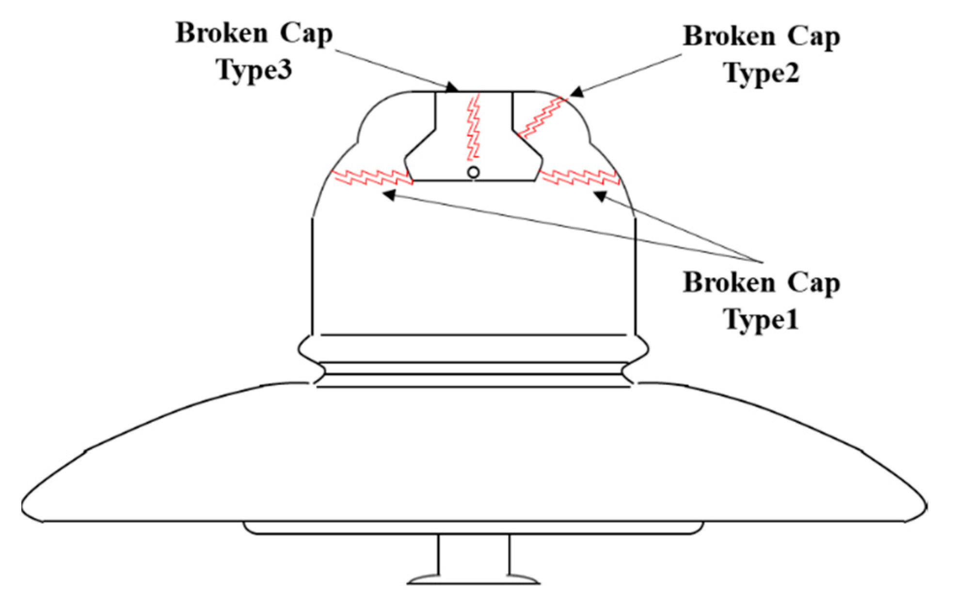
Figure 1. Porcelain insulator showing possible defects.
Applsci 10 02820 g001
Figure 2. Developed equipment and experimental setup.
Applsci 10 02820 g002
Figure 3. Frequency response function (FRF) test method using developed equipment.
Applsci 10 02820 g003
Figure 4. FRF results from the impact of porcelain. (a) FRF results of normal and cap damage; (b) FRF result of 5 to 10 kHz at normal C.
Applsci 10 02820 g004
Figure 5. Comparison of time, FFT, and FRF results by the impact of the cap: (a) time domain of normal and damaged cap specimens; (b) FFT domain of normal and damaged cap specimens; and (c) FRF domain of normal and damaged cap specimens.
Applsci 10 02820 g005
Figure 6. Division of frequency range for feature extraction.
Applsci 10 02820 g006
Figure 7. Procedure of feature extraction from experiment of developed equipment.
Applsci 10 02820 g007
Figure 8. Procedure of the bagging method from an input sample.
Applsci 10 02820 g008
Figure 9. Procedure of the discriminant analysis method from an input sample.
Applsci 10 02820 g009
Figure 10. Extraction of principal component using neighborhood component analysis (NCA) for set A: (a) lbfgs; (b) Minibatch-lbfgs; (c) sgd.
Applsci 10 02820 g010
Figure 11. 2D plot according to division of frequency range using principal component: (a) feature set A (0–10 kHz); (b) feature set B (0–4 kHz); (c) feature set C (4–10 kHz); (d) feature set D (4–7 kHz); (e) feature set E (7–10 kHz).
Applsci 10 02820 g011
Figure 12. Analysis of post-distribution area using machine learning methods: (a) support vector machine (SVM) classification; (b) bagging classification; (c) k-nearest neighbor (kNN) classification; (d) discriminant analysis (DA) classification.
Applsci 10 02820 g012
Figure 13. Heatmap chart of prediction results using developed machine learning classifiers: (a) the heat map result of the SVM classifier; (b) the heat map result of the bagging classifier; (c) the heat map result of the kNN classifier; (d) the heat map result of the DA classifier.
Applsci 10 02820 g013
Figure 14. Reanalysis based on the location of the classified data: (a) selection of median and boundary and unusual data for each material; (b) comparison of PC1 and PC2 values of selected A1–3 and C1–4 data; (c) FRF comparison of median and boundary data from normal cristobalite data; (d) FRF comparison of median and unusual data from normal alumina data.
Applsci 10 02820 g014
Table 1. Categorization of specimens according to type of material and defect.
CategorizationCristobaliteAluminaSum
Total632588
Normal592281
Defect typeSub total437
Cap336
A. P1-1
Table 2. Performance of the four learners in terms of time, accuracy, precision, recall and F1 score.
TimeAccuracyPrecisionRecallF1 Score
SVM0.074490.91%90.35%85.14%87.67%
Bagging0.250195.45%96.88%96.88%96.88%
KNN0.092690.91%89.76%85.85%87.76%
DA0.080989.77%89.84%84.00%86.82%