Article

GBSVM: Sentiment Classification from Unstructured Reviews Using Ensemble Classifier

1
Department of Computer Science, Khawaja Fareed University of Engineering and Information Technology, Rahim Yar Khan 64200, Pakistan
2
Department of Information and Communication Engineering, Yeungnam University, Gyeongsan 38541, Korea
3
Department of Computer Science & Information Technology, The Islamia University of Bahawalpur, Bahawalpur 63100, Pakistan
*
Author to whom correspondence should be addressed.
These authors contributed equally to this work.
Appl. Sci. 2020, 10(8), 2788; https://doi.org/10.3390/app10082788
Submission received: 9 March 2020 / Revised: 10 April 2020 / Accepted: 14 April 2020 / Published: 17 April 2020

Abstract

:
User reviews on social networking platforms like Twitter, Facebook, and Google+, etc. have been gaining growing interest on account of their wide usage in sentiment analysis which serves as the feedback to both public and private companies, as well as, governments. The analysis of such reviews not only plays a noteworthy role to improve the quality of such services and products but helps to devise marketing and financial strategies to increase the profit for companies and customer satisfaction. Although many analysis models have been proposed, yet, there is still room for improving the processing, classification, and analysis of user reviews which can assist managers to interpret customers feedback and elevate the quality of products. This study first evaluates the performance of a few machine learning models which are among the most widely used models and then presents a voting classifier Gradient Boosted Support Vector Machine (GBSVM) which is constituted of gradient boosting and support vector machines. The proposed model has been evaluated on two different datasets with term frequency and three variants of term frequency-inverse document frequency including uni-, bi-, and tri-gram as features. The performance is compared with other state-of-the-art techniques which prove that GBSVM outperforms these models.

Graphical Abstract

1. Introduction

With the wide proliferation of smartphones, recent years have seen the inception and expansion of social platforms like Twitter, Facebook, and Google+, etc. which collectively are referred to as ‘social media’. With its growth, social media has become one of the interactive technologies that promote users to create ideas and share information and opinions in the form of expressions or reviews. Such expressions are full of information that serves as the user’s feedback and can be utilized to revise and devise policies to improve the quality of both products and services. However, the extraction of users’ opinions from the reviews is not a trivial task. A specialized field called ‘sentiment analysis’ [1] offers a variety of techniques and tools that are used for identifying and extracting subjective information which represents users’ opinions. These techniques and tools are categorized under the natural language processing [2]. The mining of users’ opinions from user reviews is called opinion mining and is practiced within text mining. Opinion mining aims to contrive a system which is used to extract and classify review and identify opinions within the text.
Traditionally sentiment analysis classifies the opinions polarity into positive, negative and neutral classes [3]. The polarity is based on the emotions or specialized words that are present within users’ reviews. These reviews possess a significant meaning for the public, as well as, private companies because of the information they contain. The reviews contain the likes and dislike about a particular product or service so hold potential information that can be used by companies to improve the quality of the products. It can further help to devise or revise policies about particular products. The textual comments are much more significant than the numeric score because they represent what people exactly comment about a particular product [4].
Even though this content is meant to hold meaningful information for governments, businesses, and individuals, this user-generated bulk content has to be processed using text mining techniques and sentiment analysis. However, this process is not a trivial task and sentiment analysis faces several challenges that become obstacles in analyzing the accurate interpretation and meaning of sentiments and detecting the suitable sentiment polarity [5]. The first challenge is to tackle the nature of reviews text which can be either semi- or unstructured. Since most of the users writing reviews are novice or non-expert and non-professional writers, so they do not follow any set rules to express their views which results in semistructured and unstructured data [6]. Similarly, domain dependence, review structure, and language semantics make the analysis more challenging. For a more detailed list of sentiment analysis challenges users are referred to [5].
Supervised, as well as unsupervised, machine learning techniques have been applied for sentiment analysis which extracts the meaningful information from structured and unstructured text data to aid the decision-makers. Supervised techniques have proven to be more effective in determining the polarity of the sentiments, however, they require large amounts of labeled data which is not easy to get [7]. On the contrary unsupervised techniques, though not superior, are still advantageous as they can work without the labeled data. Support Vector Machine (SVM), Naive Bayes (NB), and tree-based approaches are reported to show good performance in sentiment analysis [8]. The selection of appropriate feature set from the data is an equally important step like the classification model. Term Frequency (TF), Term Frequency-Inverse Document Frequency (TF-IDF), word2vec, and parts of speech, etc. are among the most widely applied features in sentiment analysis. The use of a specific feature with different classification models show different results, so, an appropriate strategy would be to investigate the use of different features with a variety of classifiers and analyze their performance. Research works [3,7] report superior performance of uni- and bi-gram features in sentiment classification. Even so, a dedicated classifier is not suitable for tweets and often a combination also called voting or ensemble of multiple classifiers proves to show excellent performance for sentiment analysis [9].
This paper first investigates the performance of various machine learning supervised models and then contrive a voting classifier to perform sentiment analysis on a Twitter dataset. Major contributions of this study are summarized as follows:
  • Performance analysis of SVM, Gradient Boosting Machine (GBM), Logistic Regression (LR), and Random Forest (RF) is carried out for sentiment analysis. The polarity of Google apps dataset is divided into positive, negative, and neutral classes for this purpose.
  • A voting classifier, called Gradient Boosted Support Vector Machine (GBSVM), is contrived to perform sentiment analysis that is based on Gradient Boosting (GB) and SVM. The performance is compared with four state-of-the-art ensemble methods.
  • The use of TF and TF-IDF is investigated, whereby, uni-gram, bi-gram, and tri-gram features are used with the selected classifiers, as well as, GBSMV to analyze the impact on the sentiment classification accuracy.
The rest of the paper is organized in the following manner. Section 2 discusses important research works related to the current study. Section 3 outlines the details of the proposed voting classifier and describes the dataset used for the experiment. Section 4 is about the results of the experiment and discussions. Performance analysis of the proposed GBSVM is also made with other state-of-the-art models in the same section. In the end, conclusion and future work are given in Section 5.

2. Literature Review

Data over the internet is growing constantly and so does people’s choice to express their opinions. With the expansion of social platforms, tools to obtain people opinion has been changed and fields like opinion mining and sentiment analysis have received an increased demand. Owing to the potential impact that users’ opinions can make on businesses, the importance of online reviews cannot be underestimated. Consequently, a large number of research professionals are building systems that can extract the information from such reviews to benefit marketing analysis, drive public opinion, and increase customer satisfaction. As a result, sentiment analysis has been adopted and deployed in a large number of research areas and businesses.

2.1. Review Classification Using Sentiment Analysis

Authors in [10] perform sentiment analysis on data containing reviews about different electronic products such as mobiles, laptops, and monitors, etc. User reviews are collected from Twitter for this analysis. A feature vector is created to handle emotional and misspelled keywords from the text. Feature extraction is done in two steps: first, all the Twitter-specific features including hash-tags and emoticons are extracted and added to the feature vector, after that, these features are removed from the tweets and uni-gram features are extracted from tweets. For classification SVM, Naïve Bayes (NB) and maximum entropy models are used which show very similar accuracy for tweet classification into positive, negative and neutral classes. Similarly, authors in [11] performed sentiment analysis on Facebook posts. The research aimed at classifying the sentiments of students by analyzing the text that students posted on Facebook. Sentiments polarity is classified as positive, negative or neutral. Authors developed an application called SentBuk that retrieves users’ posted messages including textual messages, comments, and likes, etc. on Facebook. Sentiment classification is based on a hybrid technique that combines the lexical and machine learning approach, whereby, the lexicon-based approach is used for pre-processing while the machine learning approach is applied at the classification level. The proposed approach achieves an accuracy of 83% and is very helpful to guide teachers of the students’ current state of mind and support adaptive e-learning.
Opinion mining is very important for analyzing public opinions about a specific product and predicting its future sale trends, so, many research contributions can be found which are dedicated to mining user reviews about products. For example, authors in [3] proposed a method of extracting the polarity of users’ sentiments about products. They develop a method that can automatically discover positive, negative, and neutral reviews about any given product. The approach uses self-tagged reviews as the training data. The data chosen for testing is extracted from Amazon and C|net and provides quantitative and binary ratings. Authors suggest that metadata substitutions and variable-length features can increase the machine learning classifiers’ accuracy. In the same way, authors in [12] perform sentiment analysis on Twitter tweets to check the effect of the average person’s tweets on the fluctuation of stock prices of a multinational firm Samsung Electronics Ltd. The research presents an algorithm to give fast and accurate results for user sentiments based on the tweets. The proposed algorithm involves calculating the sentiment score based on the keywords found in the tweets and assigning a sentiment score to each tweet, whereby, the score can be 1, 0 or −1 for positive, neutral and negative, respectively. Opinion mining is not limited to analyze the reviews for products alone, but it can be applied to predict users’ sentiments in reaction to various events. For example, research [13] uses sentiment analysis on twitter reviews to predict public reaction about various events that occurred in the FIFA world cup 2014. Manually labeled data is used for training which is then used to find the correlation between the Twitter sentiment and a particular event. The model used is a Bayesian logistic regression that uses lexicons, uni-, and bi-gram features to detect subjective or objective tweets. The tweets are processed to represent the public sentiments towards unexpected events.
Another research [14] proposes a novel approach based on SentiWordNet to carry out opinion mining using web data. The count of the score falls under seven categories: strong-positive, positive, weak-positive, neutral, weak-negative, negative, and strong-negative to test the efficacy of NB, SVM, and multi-layer perceptron. The proposed approach is evaluated on movie and product web domains and results are compared against the performance of the selected classifiers. Results demonstrate that the proposed approach outperforms the selected machine learning classifiers.

2.2. Sentiment Analysis for Different Languages

Sentiment analysis faces numerous challenges on account of the use of various languages used in tweets and reviews and hence many research works are focused on analyzing within the domain of a particular language. For example, research [15] performed sentiment analysis on Arabic text. An Arabic dataset is used that has been labeled through crowdsourcing. Ten-Fold cross-validation is used for splitting the data into train and test. Machine learning techniques including K Nearest Neighbor (KNN), NB, and SVM are used for detecting the polarity of given reviews. Results show that SVM gives the best precision which is 75% and KNN gives the best recall which is 69%. Similarly, authors in [16] perform sentiment analysis on Vietnamese text. The research proposed an approach for extracting and classifying Vietnamese text into various sentiments. The semi-supervised learning approach General Knowledge-Latent Dirichlet Allocation (GK-LDA) performs better than the traditional topic modeling LDA. The superior performance is on account of a dictionary-based approach that extracts noun-phrases rather than merely extracting word seeds.
In the same manner, research [17] conducted a sentiment analysis of the Thai language. Because the Thai language is a non-segmented language where the texts are made in a long sequence of characters without word boundaries, so, traditional Bag-of-Words (BoW) approaches are not suitable for Thai text. The proposed approach is a machine learning-based approach where ORCHID, a Thai word-segmented text corpus, is used. Later, Thai stopwords are removed before the emotions word tagging can be done. Then sentiment level is assigned to reviews based on the detected emotional word. The proposed approach helps companies know the weaknesses of their products based on the analysis of the user reviews. In another research [18] sentiment analysis is performed on different languages reviews such as English, Dutch, and French. Reviews are collected from the World Wide Web and classification is performed using SVM, multinomial NB and Maximum Entropy Classifier (MEC). For feature selection uni-grams and BSubjectivity, bi-grams, and adjectives are used. Uni-gram and BSubjectivity gives the most accurate results of 86% with SVM and 87% with MEC.

2.3. Research Works on the Pre-Processing in Sentiment Analysis

The tweets and reviews used for sentiment analysis often contain noise in the form of words that do not contribute towards the classification and hence pre-processing is an important task in sentiment analysis. For example, research [19] employs sentiment analysis on Arabic tweets. The impact of stemming, feature correlation, and n-grams model is thoroughly investigated in Arabic text. Then, three classifiers SVM, NB, and KNN are evaluated for their effectiveness to perform the sentiment analysis on Arabic text. Results show that the selection of an appropriate pre-processing strategy is very critical to achieve higher performance. Likewise, authors in [20] suggest that pre-processing is an important task, as it can substantially improve the classification and accuracy. Besides, research [21] proves that an appropriate pre-processing phase can elevate the performance of machine learning classifiers. Feature selection is another important task in sentiment analysis which can dramatically improve classification accuracy. Authors in [22] proposed a novel filter-based probabilistic feature selection method called the Distinguishable Feature Selection (DFS) method that is used for text classification. Results show that DFS gives competitive results to other feature selection techniques.
Despite various methods proposed and used for sentiment analysis, there is still room for improvement, as no method is suitable for all kinds of data. Specifically, the machine learning models show variant performance when used with a specific pre-processing strategy and particular feature selection method. Voting classifiers proved to show superior performance than single classification models, as in [9], where a voting classifier based on LR and Stochastic Gradient Descent Classifier (SGDC) is used for tweet classification. As a consequence, this research aims at devising a Voting Classifier (VC) which can perform better than already proposed models to predict sentiments polarity from unstructured text.

3. Materials and Methods

This section provides the details of the proposed approach, the dataset used for the experiment, feature selection, selected machine learning classifiers and the accuracy metrics used to evaluate the performance. The proposed approach is based on GBM and SVM, so it is highly desirable to describe how these models work before the narration of the proposed approach. The following section discusses the machine learning classifiers selected for the experiments as well as GBM and SVM used for the proposed voting classifier.

3.1. Classifiers Selected for the Experiment

Machine learning models have shown good performance for sentiment classification. A variety of machine learning models are available that can be used for sentiment prediction and many of these models have been implemented in SciKit learn [23]. For the current study, we used the SciKit learn stable version 0.22.0. This study considers the use of ensemble models for sentiment classification on account of their superior performance. Researches [24,25] proves that ensemble methods can substantially elevate the performance of individual base learners for sentiment classification and hence are favorable to use for sentiment analysis. The ensemble methods are meta-algorithms that combine several machine learning techniques into one predictive model which decreases variance(bagging) and bias (boosting) to obtain improved predictions(stacking) [26]. Supervised machine learning classification approaches involve building classifiers from labeled instances of texts or sentences.

3.1.1. Random Forest

RF is an ensemble model used both for classification and regression [27]. It trains multiple trees where each tree is built using a random subset of the vector features. The decisions of each tree are combined using a voting algorithm that gives the result. The sequence of features and the value of the feature generates the path to a leaf that represents the decision. While training, the values of the intermediate nodes are updated to minimize a cost function that evaluates the performance of the trees. RF reduces variance in different ways; firstly on training different samples of data and secondly by using a random subset of different features [28]. This study uses the RF implementation provided by SciKit learn.

3.1.2. Logistic Regression

LR performs predictive analysis and is used to describe data and explain the relationship between one dependent binary variable and one or more nominal, ordinal, interval or ratio-level independent variables. LR is a statistical machine learning algorithm that classifies the data by considering the output variables on extreme ends and tries to make a logarithm line that distinguishes between them [29]. This model is not only used for regression but also the classification task. It is one of the machine learning algorithms that provide low variance and great efficiency. A logistic model can be updated easily with new data using stochastic gradient descent.

3.1.3. Gradient Boosting Machine

GBM is a machine learning technique used for regression and classification problems and produces a prediction model in the form of an ensemble of weak prediction models, typically decision trees [30]. It builds the model in a stage-wise fashion as other boosting methods do, and generalizes them by allowing optimization of an arbitrary differentiable loss function. In supervised learning, boosting is a method of converting weak learner into a strong learner. In boosting each new tree is a fit on a modified version of the original dataset. It has shown considerable success for practical applications in machine learning tasks [30,31]. A loss function in GBM is to be minimized to improve its performance. The gradient descent is the most widely used loss function and has the form:
y i p = y i p α ( y i y i p ) ,
where α represents the learning rate which can be varied between 0 and 1 to tune the performance of GBM, and  ( y i y i p ) shows the sum of the residuals. The loss function is a measure that indicates the efficiency of coefficients of a model that fit the underlying data. A logical understanding of loss function would depend upon what we are trying to optimize [32]. The architecture of a GBM is given in Figure 1.
GBM is not only useful in practical applications, but it also has significant usage in data mining challenges [33,34]. The functionality of GBM is described in Algorithm 1.

3.1.4. Support Vector Machine

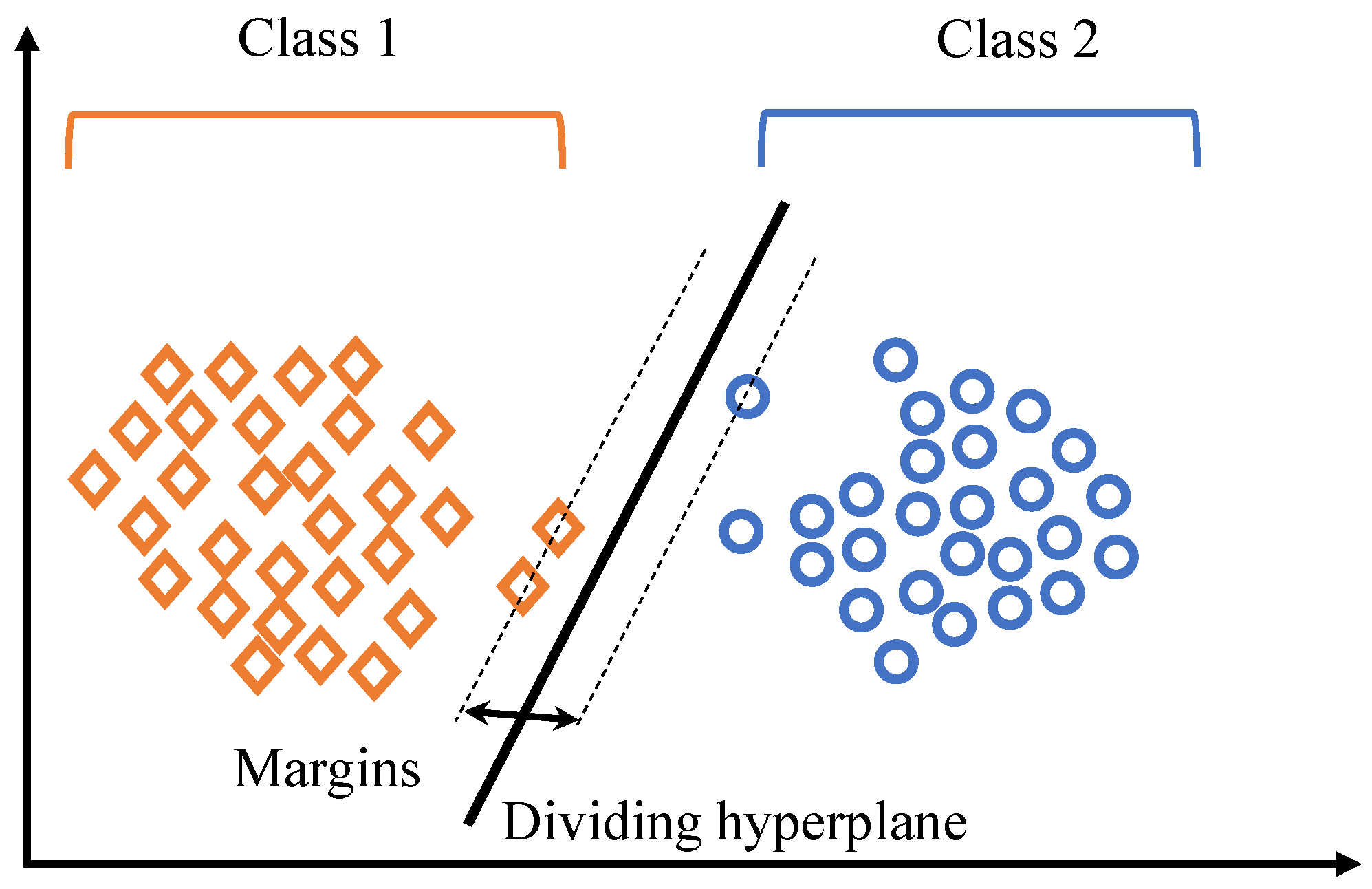
SVM was originally developed by Cortes and Vapnik for binary classification [35]. It is a non-probabilistic binary linear classifier that constructs a hyperplane or set of hyperplanes high or infinite-dimensional space, which can be used for classification, regression, and similar other tasks [36,37]. An SVM uses a device called kernel mapping to map the data in input space to a high-dimensional feature space in which the problem becomes linearly separable [38]. The basic idea underlying the SVM for sentiment classification is to find a hyperplane that divides the documents, or in our case, Google app reviews as per the sentiment and the margin between the classes (positive, negative and neutral) being as high as possible. The points that lay on the separation boundaries are called support vectors, as shown in Figure 2.
Algorithm 1 Friedman’s Gradient Boosting Algorithm [31].
Inputs:
  • input data ( x , y ) i = 1 N
  • number of iterations M
  • choice of the loss-function Ψ ( y , f )
  • choice of the base-learner model h ( x , θ )
1:
initialize f ^ 0 with a constant  
2:
for t = 1   t o   M do
3:
    compute the negative gradient g t ( x )  
4:
    fit a new base-learner function h ( x , θ t )   
5:
    find the best gradient descet step-size ρ t
     p t = a r g m i n ρ i = 1 N Ψ { y i , f ^ t 1 ( x i ) , ρ h ( x i , θ t ) }  
6:
    update the function estimate:
     f ^ t f ^ t 1 + ρ t h ( x , θ t )  
7:
end for 
The class separability depends upon the distance between the samples of the classes. In other words, the higher the distance between the support vectors (margins) is, the more distinguished the classes are. The hyperplanes are originated using quadratic programming optimization problem [39]. The decision function of an SVM is related not only to the number of SVs and their weights but also to the a priori chosen kernel that is called the support vector kernel [40,41]. For this purpose, various kernels like radial, polynomial, and neural kernels, etc., are used with SVM [42]. The working principle of SVM is given in Algorithm 2 [43,44].

3.2. Proposed Approach

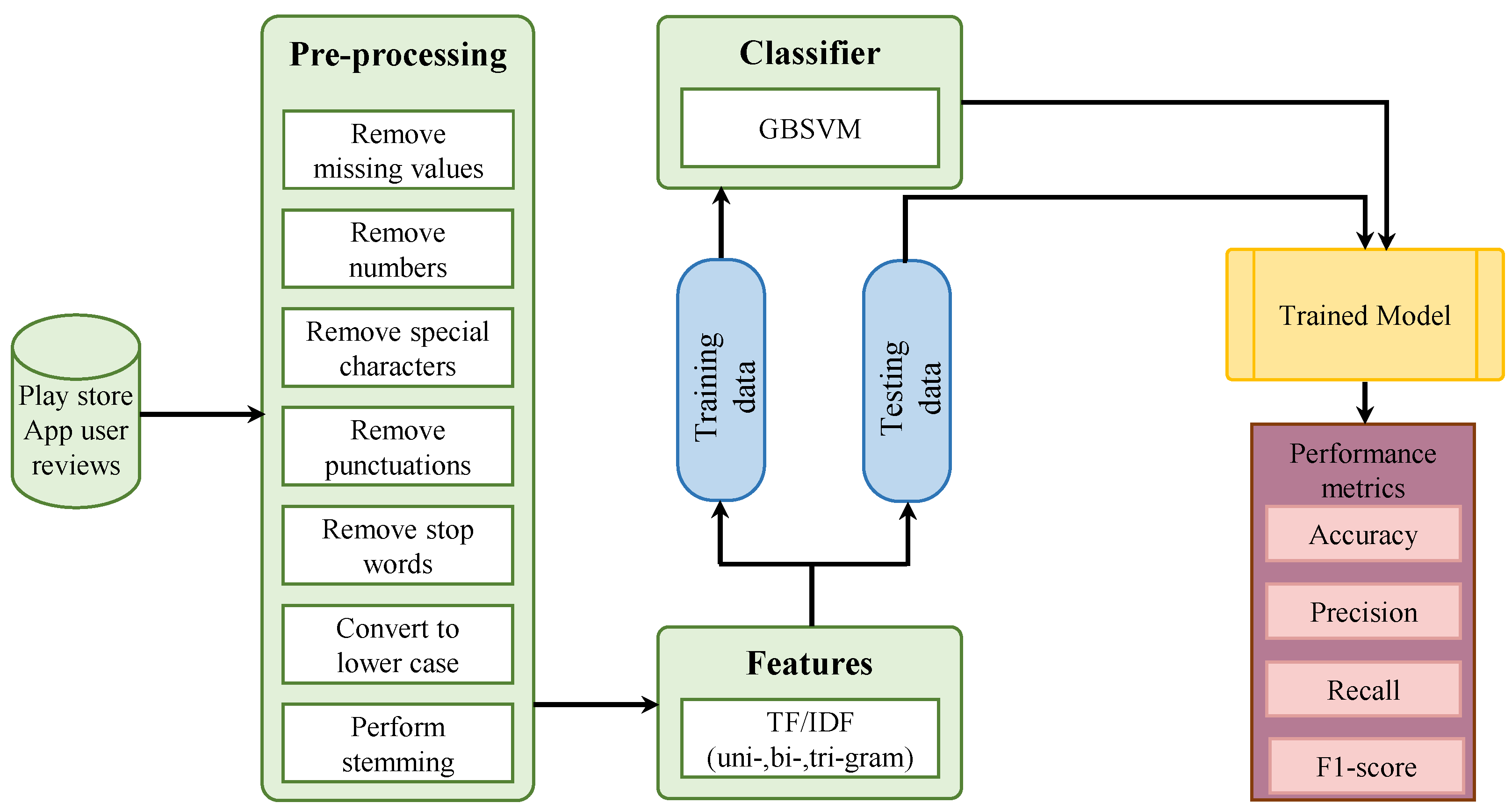
In this section, GBSVM a novel approach is introduced for sentiment classification and prediction of review sentiments of Google play store apps. The purpose of the proposed approach is to perform a multi-class sentiment classification on the unstructured data. Figure 3 shows the diagram for the proposed methodology.
Algorithm 2 Support voting machine.
Input: input data ( x , y ) i = 1 N
1:
for i = 1   t o   M do
2:
    closest_ pair= m i n 1 2 | | ω | | 2 + C i ( ρ i + ρ i )  
3:
    if closest_ pair==minimum then
4:
          for j = 1   t o   n do
5:
              decision_ function_ to_ draw_ hyperplane s i g n ( i a i z i ( x ) )  
6:
              optimization of hyperplane to classify the data according to classes  
7:
              set the optimal margin ω ( a , a ) = i ( a i a i ) z i  
8:
        end for 
9:
    end if 
10:
end for 

3.2.1. Data Pre-Processing

Before describing the proposed approach, we would like to briefly explain the pre-processing followed for the experiments conducted to evaluate the performance of both the proposed approach, as well as, the selected machine-learning classifiers. Often the dataset contains noise in the form of unnecessary data that does not contribute towards the classification and needs to be cleaned. Data pre-processing is the process used for removing noisy and incomplete data. Pre-processing plays a pivotal role to improve classification accuracy [21]. The dataset used in this study contains a large amount of unnecessary data that does not play any role in the prediction. Since training and testing time increases when the dataset is larger, so, removing un-necessary data can speed up the training process as well. Pre-processing involves the steps carried out to clean the data so that the learning efficiency of the models can be enhanced. For this purpose, the natural language tool kit (NLTK) of Python has been utilized. It is a suite of text processing libraries that can be used for a variety of processing tasks and we used NLTK 3.5b1 with Python 3 [45]. Figure 4 shows the pre-processing steps that are followed in the current study.
As a first step, all the reviews with missing values are identified and removed as the missing data can degrade the performance of the classifiers. Next, numerical values are removed from the text as they do not contribute towards the learning of the classifiers. It decreases the complexity of the training classifiers. Occasionally, reviews contain special symbols like a hear sign, thumb sign, etc. that need to be removed to reduce feature dimension and improve performance. After that the following punctuation []() /|, ; . ’ is removed from the reviews in view of the fact that it does not contribute to the text analysis. It cripples the model’s ability to discriminate between punctuation and other characters.
As a next step, words are converted to lowercase because the text analysis is case sensitive. If this step is not carried out, the machine learning models will count for example ‘Excellent’ and ‘excellent’ as two different words which will ultimately affect the classifier’s performance [46]. In the end, stemming is performed. It is a very important pre-processing step that removes the affixes from the words. It transforms the extended words into their base forms. For example, ‘loves’, ‘loved’, and ‘loving’ are the modified forms of ‘love’. Stemming changes these words into the original/root form and helps to increase the performance of a classifier [47].

3.2.2. Proposed GBSVM

The proposed classifier is an ensemble model also called a meta-classifier that performs classification by combining the probability scores from different base models. The final predicted class is based on the aggregate results from the base models. The VC (GBSVM) presented in this study is the ensemble of two classifiers GBM and SVM which are used for the final prediction of the target class. GBM is an efficient algorithm that uses a boosting method that converts the weak learner into a strong learner and trains many models in a gradual and sequenced manner. GBM is the extended version of a decision tree algorithm, that does not work well because it generates random trees and one tree has no co-relation with the other, i.e., it builds random independent trees. While the trees in the GBM are built to eliminate the short-coming (error-residuals) of the previous weak tree.
The SVM, on the contrary, is a linear model used to solve classification and regression problems. It deals with both linear and non-linear problems and works well for different applications [48]. SVM separates data into different classes by using a line or hyper-plane. SVM can perform complex types of classification based on the labels provided to the algorithm. A kernel is used in SVM that converts the low-dimension spaces into high-dimension spaces as it converts the problems into separate problems that are not separable.
The final result from the VC can be based on either the hard voting or soft voting. Hard voting is a case of majority voting where the class prediction from each based model is considered. Here, the class label Y ^ can be predicted by majority voting of each classifier C.
Y ^ = m o d e [ c 1 ( x ) , c 2 ( x ) , , c m ( x ) ] .
For example, if the predictions from c 1 , c 2 , and  c 3 are ‘positive’, ‘negative’, and ‘positive’, respectively, then the final prediction will be ‘positive’ by the majority vote.
Y ^ = m o d e [ p o s i t i v e , n e g a t i v e , p o s i t i v e ] = p o s i t i v e .
The soft voting, on the other hand, considers the probability score from each classifier of a specific class that the current sample belongs to. At that point, soft voting criteria determine the class with the highest probability which it gets by averaging the individual values of the classifiers [49].
The proposed GBSVM takes the advantage of the advantages of both GBM and SBM and combines their predicted probability of a particular class to make the final decision. M G B M and M S v M are trained on the training data set and then used to predict the probability for positive, neutral and negative classes separately. Using the predicted probability from the two classifiers, an average probability for each class is computed for a given review. The decision function is then used to decide the final prediction/label of the review which is based on the highest average probability for a class. The working mechanism of the GBSVM is given in Algorithm 3.
Algorithm 3 Gradient Boosted Support Vector Machine (GBSVM).
Input: input data ( x , y ) i = 1 N
M G B M = Trained_ GBM
M S V M = Trained_ SVM
1:
for i = 1   t o   M do
2:
    if M G B M 0 & M S V M 0 & t r a i n i n g _ s e t 0 then
3:
         P r o b S V M P o s = M S V M . p r o b i b i l i t y ( P o s c l a s s )  
4:
         P r o b S V M N e u = M S V M . p r o b i b i l i t y ( N e u c l a s s )  
5:
         P r o b S V M N e g = M S V M . p r o b i b i l i t y ( N e g c l a s s )     
6:
         P r o b G B M P o s = M G B M . p r o b i b i l i t y ( P o s c l a s s )  
7:
         P r o b G B M N e u = M G B M . p r o b i b i l i t y ( N e u c l a s s )  
8:
         P r o b G B M N e g = M G B M . p r o b i b i l i t y ( N e g c l a s s )   
9:
         Decision function = m a x ( 1 N c l a s s i f i e r c l a s s i f i e r ( A v g ( P r o b S V M P o s , P r o b G B M P o s ) , A v g ( P r o b S V M N e u , P r o b G B M N e u ) , A v g ( P r o b S V M N e g , P r o b G B M N e g ) ) )  
10:
    end if 
11:
    Return final label p ^  
12:
end for 
In this study, the soft voting technique is used. The VC in the current study is expressed as:
p ^ = a r g m a x { i n G B M i , i n S V M i } .
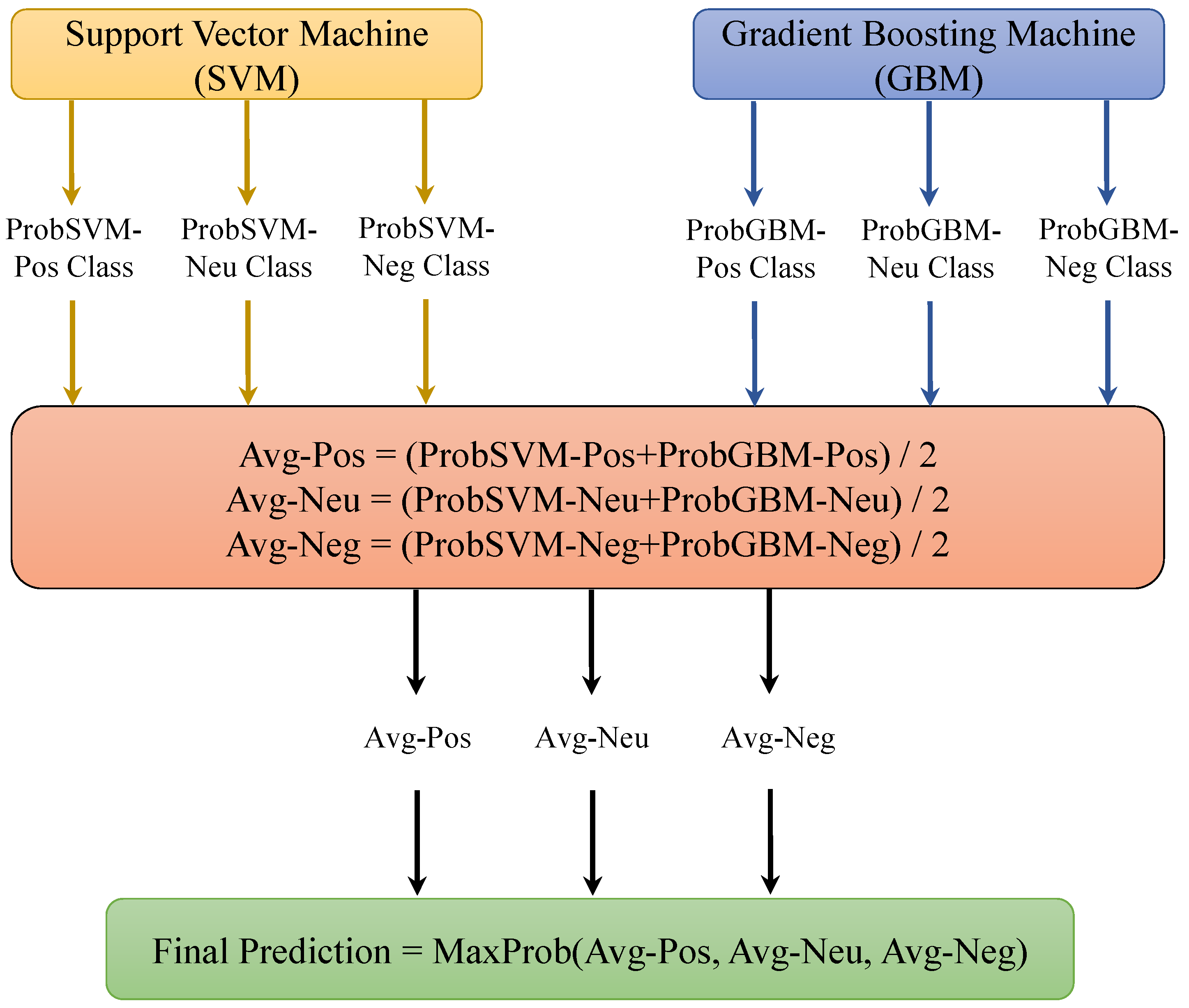
Here i n G B M i and i n S V M i both will give prediction probabilities against each test example. After that, the probabilities for each test example by both GBM and SVM passes through the soft voting criteria as shown in Figure 5.
When a given sample passes through the SVM and GBM, they give the probability score against each class (positive, negative, neutral). Let GBM’s probability score be 0.96696002, 0.02426578, 0.0087742, and for P r o b G B M P o s , P r o b G B M N e u , and P r o b G B M N e g classes and SVM’s predicted probabilities be 0.997757249, 0.00206882765, and 0.000173923303 for P r o b S V M P o s , P r o b S V M N e u , and P r o b S V M N e g , respectively. Then the average probability for the three classes can be calculated as
Avg-Pos = (0.96696002 + 0.997757249)/2 = 0.9823586345
Avg-Neu = (0.02426578 + 0.00206882765)/2 = 0.013167303825
Avg-Neg = (0.0087742 + 0.000173923303)/2 = 0.0044740616515
Since the final prediction is the M a x P r o b ( A v g P o s , A v g N e u , A v g N e g ) , which in this case is for the positive class, so the final predicted class is ‘positive’ and the actual class of the sample review is also positive in the dataset.

3.3. Dataset

Dataset plays a very important role to perform the sentiment analysis. This study utilizes the dataset that contains the mobile application reviews for Google apps. The dataset used in the current study has been downloaded from and is freely available at [50]. The dataset contains user reviews about Google apps in the English language. It contains 64,295 records consisting of attributes including ‘App’, ‘Translated_ Reviews’, and ‘Sentiments’. The description of the dataset attributes is given in Table 1.
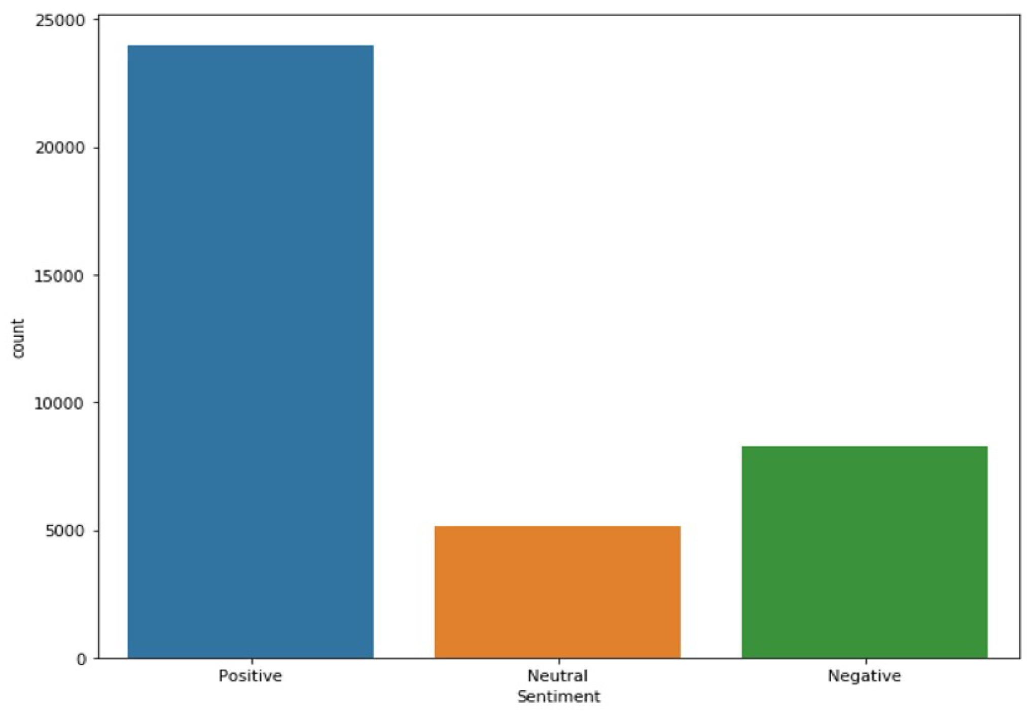
The dataset contains names of different apps and ‘translated_ reviews’ attribute shows users reviews against the individual app. There are three classes in sentiments attribute namely positive, negative and neutral. Figure 6 shows the distribution of positive, negative and neutral reviews. There are 23,998 positive reviews, 8271 negative and 5158 neutral reviews in the dataset.

3.4. Feature Selection

Feature selection is a method of selecting the subset of relevant features for model construction, thus reducing the training time of models, simplifying the models and improving the probability of generalization and avoid overfitting. In feature extraction, input raw data are transformed into features. Supervised machine learning algorithms require text data in the form of vectors for model training. So extraction and conversion of text data into features are required without losing any important information. There is a large variety of features that have shown promising results in the classification, e.g., BoW (Bag of Words), word2vec, and TF, etc. BoW is the representation of the given text into vectors of fixed length. It does so by counting the occurrence of each word in a given text, i.e., it gives the numbers to each word is [51]. The BoW, however, is not as efficient as TF or TF-IDF are on account of its inability to capture the semantics of documents [52]. Word2vec feature extraction is based on a two-layer neural network that is used to extract feature vectors from a text corpus. It uses either CBoW (Continuous BoW) or the SG (Skip-Gram)model to do that [53]. This study considers TF and TF-IDF with its variants [54]. TF counts the frequency of words in the document i.e., it converts a collection of a text document into a matrix of occurrences of each word in the document.
Other than TF, this study considers TF-IDF with bi- and tri-gram [54] for feature selection. Even though humans can understand a language easily, it is often very complicated to train a model on the text. For this purpose, various patterns or features are used to train a model. Words convey a different meaning when considered alone than when they are joined with other words. A word if considered alone is called a uni-gram and independent of other words, for example, ‘one great app’ has three uni-grams including ’one’, ’great’, and ’app’. N-gram refers to N sequence of items for a given sample where N can be 1, 2, 3, etc. For example for the above-mentioned sentence, bi-gram would be ’one great’, and ’great app’. N-gram features are reported to show better performance for review classification [55,56]. TF-IDF weighs down the most common words occurring in all text documents and gives importance to each word that appears in a subset of documents. It is a well-known algorithm that is used to transform the text into a feature vector. TF-IDF works by assigning lower weights to most common words but giving importance to rare words in a document and converts the text into a vector form. This technique is used for feature extraction in various NLP applications. TF tells which term feature is most important in a given document, while IDF presents how many documents contain that term.

3.5. Performance Evaluation Parameters

A large variety of metrics are available that can be used to evaluate the performance of classifiers [57], however, four of them are among the widely used parameters including accuracy, precision, recall, and f1-score. Four basic terms that need the understanding to grasp the performance evaluation metrics are True Positive (TP), False Positive (FP), True Negative (TN), and False Negative (FN) [58]. Accuracy determines the performance of a classifier in terms of the percentage of reviews that are predicted correctly. Using the above-mentioned terms, accuracy can be calculated using:
A c c u r a c y = N u m b e r o f c o r r e c t p r e d i c t i o n s T o t a l n u m b e r o f p r e d i c t i o n s .
The recall is often referred to as the completeness of a classifier. What proportion of actual positive is identified correctly is given by recall. It is also called the sensitivity and can be calculated using the following formula:
R e c a l l = T P T P + F N .
Precision shows the exactness of a classifier. It shows what percentage of all samples are labeled positive that are actually positive. It is calculated with the following equation:
P r e c i s i o n = T P T P + F P .
The F score is a statistical analysis measure that takes both the precision and recall into account and computes a score between 0 and 1. The closer the value is to 1, the higher the accuracy of the classifier will be. F1 is calculated as:
F 1 = 2 R e c a l l × P r e c i s i o n R e c a l l + P r e c i s i o n .

3.6. Experiment Settings

Selected machine learning classifiers, as well as, the proposed VC are executed to analyze the initial results and then the parameters are finely tuned to increase the performance. Empirical settings of these parameters resulted in enhanced performances from the selected classifiers. Results discussed in Section 4 are the best results that we got from these classifiers and based on the parameters shown in Table 2.
RF is executed with two parameters control: max_ depth and random_ state. The former shows the maximum depth of the tree that will be created. It can also be taken as the longest route from the node to the leaf. An optimal decision tree (DT) is known to be NP-complete in many aspects. So practical DT are heuristic where local optimal decisions are taken at each node. Hence a globally optimal decision tree is not guaranteed. So multiple trees are trained in an ensemble classifier and features are sampled randomly. The latter parameter of RF controls the random choices for such training. The C defines how much we want to avoid misclassification of each training example. For smaller values, the misclassified examples are higher and vice versa. Maximum iterations define the maximum number of iterations that we want to carry out to the optimization process. Parameter ‘tol’ refers to tolerance for stopping criterion. Penalty shows the regularization technique used for the model. L2 represents ‘Ridge Regression’ which adds ‘squared magnitude’ of coefficient as a penalty to the loss function of the model. The parameter ‘fit_ intercept’ is set ‘True’, that includes the intercept value to the regression model. ‘Solver’ parameter defines the algorithm to be used in the optimization problem which is set to ‘lbfgs’ which is necessary to handle the ‘L2’ penalty and handle the multinomial loss.
For GBM maximum depth is set to 10 while the learning rate is 0.4. The parameter ’n_ estimators’ is set to 100; it defines the number of boosting stages. Setting a larger number of estimators usually gives better performance. Cache_ size defines the size of the kernel cache (in MB). The ‘decision_ function_ shape’ defines whether to return ‘ovr’ (one-vs-rest) or ‘ovo’ (one-vs-one); we set it to ‘ovr’. For ‘degree’, we used the default value, i.e., 3; which uses 1/(n_ features * X.var()) as the value of gamma. Kernel methods enable the mapping of non-linear observations into a higher-dimensional space to make them separable. Various kernels are used in machine learning models including linear, Gaussian, neural, etc. For SVM, we used a ‘linear’ kernel that is used when the data is linearly separable. The number of iterations is set to −1 which means that there is ’no limit’ to iterations and ’shrinking’ heuristic is set to ’True’.

4. Results and Discussions

This section contains the details of the experimental results conducted in this research along with the discussion of the results. Experiments are conducted using SVM, GBM, RF and LR classifiers to classify sentiments into positive, negative and neutral classes. The train-test split is done as 70:30 for training and testing, respectively. Although the proposed GBSVM is constituted of GBM and SVM, these techniques are tested individually as well to analyze their performance. Consequently, four techniques including GBM, SVM, RF, and LR are analyzed for their efficacy against the proposed approach. For the experiments, we did not use the cross-validation. Although k-fold is more precise from a theoretical perspective, yet more computationally complex. In the light of the research [59] that states that cross-validation is the common exercise but sometimes it is better not to use it, we did not use it. TF and uni-, bi- and tri-gram variants of TF-IDF are used as features for classification. Results obtained using TF features are shown in Table 3.
Experiment results demonstrate the proposed GBSVM performs well when used with TF features. The underlying reason is the combination of GBM and SVM where GBM works on weak learners to make it strong for prediction. The learning rate applied is 0.1 which fairly gives accurate results and SVM is used with linear kernel and so performs faster and more accurately on the categorical data. As the dataset contains a higher number of positive class instances so, the precision rate for the positive class is quite good.
Similarly, GBSVM outperforms other machine learning classifiers when TF-IDF features are used for sentiment classification and gives an accuracy of 92%. Like before, precision results for the positive class are comparatively higher than that of negative and neutral classes primarily on account of the higher training data samples for positive class. F1 score which considers both precision and recall is also high for GBSVM than that of other classifiers. Results shown in Table 4 are for uni-gram TF-IDF, however, bi-gram TF-IDF has also been used and results are shown in Table 5.
Results with bi-gram TF-IDF features reveal that the performance of all classifiers has been highly degraded. Theoretically, a higher-order n-gram model contains more information on a word’s context which can lead to a model overfit. This happens when the data is sparse where we have a relatively large number of tokens but the frequency of the tokens is low. In such scenarios, a low order n-gram model can perform better than a high order n-gram model which is the case with the current dataset. This can be further corroborated from the results when TF-IDF tri-gram features are used for sentiment classification. Results with tri-gram features are shown in Table 6.
As we can see the accuracy values obtained from different classifiers have been further decreased with tri-gram features. The most probable reason is the nature of the data that has been used during the training phase. In many cases, bi- and tri-gram performs worse than uni-grams, particularly when adding extra features because it may lead to overfitting. Another reason is the small sample of training data. It is most probable that classifiers are likely to have unseen tri-grams which can reduce the performance with the test data. Often the data contains only single words that lead to better performance of uni-gram than that of bi- and tri-gram models. The selected data mostly consists of single words like ‘great’, ‘nice’, and ‘good’, etc. so training on these results in higher accuracy for classifiers when uni-gram is used and the result becomes poorer gradually if we move from bi-gram to tri-gram. That is the reason the performance of selected classifiers has been degraded, however, even so, GBSVM performs better than other classifiers.

4.1. Performance Analysis of the Proposed GBSVM

A performance comparison of the proposed GBSVM is done as well to show its performance against other similar models. Authors in [9] perform tweet classification based on user sentiments with a VC which is based on LR and SGDC. Three features have been investigated as well including TF, TF-IDF, and word2vec. The performance of VC in [9] is better with TF and TF-IDF which yields an accuracy of 78.9%, and 79.1%, respectively. The approach in [9] is tested on the selected dataset with TF-IDF uni-gram features and it achieves an accuracy of 88.01%. On the other hand, the accuracy of the proposed GBSVM is 93.0% which is much better than that of [9].
Similarly, another work [60] proposes the combination of NB, Rocchio, and KNN for text classification. This voting classifier can predict 89.23% of the samples accurately. However, when applied to the selected dataset, its accuracy is demoted to 73.0%, while at the same time GBSVM gives an accuracy of 93.0%. Results shown in Table 7 that the proposed GBSVM performs better than both [9] and [60].

4.2. Analyzing the Performance of GBSVM on Additional Dataset

Since the proposed GBSVM is tested only on one dataset, so the results cannot be generalized. To show its capability, it is tested on another dataset called ‘20 newsgroup dataset’ which consists of a total of 18,000 records and comprises of 20 classes [61]. The dataset has been experimented upon by two research works [62,63]. Research [62] utilizes a Graph Convolutional Network (GCN), and a Simple graph Convolutional Network (SGCN) for classification.
Similarly, another work [63] proposed a Neural Attentive Bag-of-Entities(NABoE) model for the classification of twenty classes in the dataset. The proposed model is a neural network model that performs text classification using the entities in the knowledge base. Results from [62,63] are compared against the proposed GBSVM and the performance is shown in Table 8. Results show that the proposed GBSVM outperforms these models and achieves higher accuracy.

5. Conclusions

The rise and widespread use of social media has opened new ways of expressing opinions and sentiments on social platforms like Twitter, Facebook, etc. It has fueled the interest in sentiment analysis, as finding correct sentiments from text has become an important tool for individuals and companies to devise and revise products and services for increased customer satisfaction. In this paper, a sentiment analysis approach is contrived which performs voting from two base models including GBM), and SV). The performance is tested against four machine learning models including GBM, SVM, LR, and RF. Experiment results on the Google app dataset show that the proposed GBSVM outperforms machine learning classifiers. Additionally, TF, and three variants of TF-IDF uni-, bi-, and tri-gram are also investigated for their suitability as classification features which reveal that uni-gram performs better than that of TF and bi- and tri-gram TF-IDF. However, these results are not conclusive as a large dataset may affect the results and the bi-gram and tri-gram perform better with a larger dataset, which is intended as future work. Refinement in the accuracy is further possible with a more balanced data where the training samples for positive, negative, and neutral are approximately similar. Performance comparison of GBSVM with four similar models show that it performs better and achieves higher accuracy.

Author Contributions

Conceptualization, M.K. and I.A.; data curation, M.A.; formal analysis, M.K. and A.M.; funding acquisition, G.S.C.; investigation, M.K.; methodology, A.M.; project administration, S.U.; software, M.A.; validation, S.U.; writing—original draft, I.A.; writing—review and editing, G.S.C. All authors have read and agreed to the published version of the manuscript.

Funding

This research was supported by Basic Science Research Program through the National Research Foundation of Korea (NRF) funded by the Ministry of Education (NRF-2019R1A2C1006159), MSIT(Ministry of Science and ICT), Korea, under the ITRC(Information Technology Research Center) support program (IITP-2020-2016-0-00313) supervised by the IITP(Institute for Information & communications Technology Promotion), and the Brain Korea 21 Plus Program(No. 22A20130012814) funded by the National Research Foundation of Korea (NRF).

Conflicts of Interest

The authors declare no conflict of interest. The funders had no role in the design of the study; in the collection, analyses, or interpretation of data; in the writing of the manuscript, or in the decision to publish the results.

References

  1. Chen, L.; Wang, W.; Nagarajan, M.; Wang, S.; Sheth, A.P. Extracting diverse sentiment expressions with target-dependent polarity from twitter. In Proceedings of the Sixth International AAAI Conference on Weblogs and Social Media, Dublin, Ireland, 4–7 June 2012. [Google Scholar]
  2. Liu, B. Handbook Chapter: Sentiment Analysis and Subjectivity. Handbook of Natural Language Processing. In Handbook of Natural Language Processing; Marcel Dekker, Inc.: New York, NY, USA, 2009. [Google Scholar]
  3. Dave, K.; Lawrence, S.; Pennock, D.M. Mining the peanut gallery: Opinion extraction and semantic classification of product reviews. In Proceedings of the 12th International Conference on World Wide Web, Budapest, Hungary, 20–24 May 2003; pp. 519–528. [Google Scholar]
  4. Kasper, W.; Vela, M. Sentiment analysis for hotel reviews. In Proceedings of the Computational Linguistics-Applications Conference, Jachranka, Poland, 17–19 October 2011; Volume 231527, pp. 45–52. [Google Scholar]
  5. Hussein, D.M.E.D.M. A survey on sentiment analysis challenges. J. King Saud Univ.-Eng. Sci. 2018, 30, 330–338. [Google Scholar] [CrossRef]
  6. Mukherjee, A.; Venkataraman, V.; Liu, B.; Glance, N. What yelp fake review filter might be doing? In Proceedings of the Seventh International AAAI Conference on Weblogs and Social Media, Cambridge, MA, USA, 8–11 July 2013. [Google Scholar]
  7. Pang, B.; Lee, L.; Vaithyanathan, S. Thumbs up? Sentiment classification using machine learning techniques. In Proceedings of the ACL-02 Conference on Empirical Methods in Natural Language Processing, Stroudsburg, Philadelphia, PA, USA, 6–7 July 2002; Association for Computational Linguistics: Shumen, Bulgaria, 2002; Volume 10, pp. 79–86. [Google Scholar]
  8. Pang, B.; Lee, L. Opinion mining and sentiment analysis. Found. Trends. Inf. Retr. 2008, 2, 1–135. [Google Scholar] [CrossRef] [Green Version]
  9. Rustam, F.; Ashraf, I.; Mehmood, A.; Ullah, S.; Choi, G.S. Tweets Classification on the Base of Sentiments for US Airline Companies. Entropy 2019, 21, 1078. [Google Scholar] [CrossRef] [Green Version]
  10. Neethu, M.; Rajasree, R. Sentiment analysis in twitter using machine learning techniques. In Proceedings of the 2013 Fourth International Conference on Computing, Communications and Networking Technologies (ICCCNT), Tiruchengode, India, 4–6 July 2013; pp. 1–5. [Google Scholar]
  11. Ortigosa, A.; Martín, J.M.; Carro, R.M. Sentiment analysis in Facebook and its application to e-learning. Comput. Hum. Behav. 2014, 31, 527–541. [Google Scholar] [CrossRef]
  12. Bakshi, R.K.; Kaur, N.; Kaur, R.; Kaur, G. Opinion mining and sentiment analysis. In Proceedings of the 2016 3rd International Conference on Computing for Sustainable Global Development (INDIACom), New Delhi, India, 16–18 March 2016; pp. 452–455. [Google Scholar]
  13. Barnaghi, P.; Ghaffari, P.; Breslin, J.G. Opinion mining and sentiment polarity on twitter and correlation between events and sentiment. In Proceedings of the 2016 IEEE Second International Conference on Big Data Computing Service and Applications (BigDataService), Oxford, UK, 29 March–1 April 2016; pp. 52–57. [Google Scholar]
  14. Ahmed, S.; Danti, A. A novel approach for Sentimental Analysis and Opinion Mining based on SentiWordNet using web data. In Proceedings of the 2015 International Conference on Trends in Automation, Communications and Computing Technology (I-TACT-15), Bangalore, India, 21–22 December 2015; pp. 1–5. [Google Scholar]
  15. Duwairi, R.M.; Qarqaz, I. Arabic sentiment analysis using supervised classification. In Proceedings of the 2014 International Conference on Future Internet of Things and Cloud, Barcelona, Spain, 27–29 August 2014; pp. 579–583. [Google Scholar]
  16. Le, H.S.; Van Le, T.; Pham, T.V. Aspect analysis for opinion mining of Vietnamese text. In Proceedings of the 2015 International Conference on Advanced Computing and Applications (ACOMP), Ho Chi Minh City, Vietnam, 23–25 Novomber 2015; pp. 118–123. [Google Scholar]
  17. Chumwatana, T. Using sentiment analysis technique for analyzing Thai customer satisfaction from social media. In Proceedings of the 5th International Conference on Computing and Informatics (ICOCI), Istanbul, Turkey, 11–13 August 2015. [Google Scholar]
  18. Boiy, E.; Moens, M.F. A machine learning approach to sentiment analysis in multilingual Web texts. Inf. Retr. 2009, 12, 526–558. [Google Scholar] [CrossRef]
  19. Duwairi, R.; El-Orfali, M. A study of the effects of preprocessing strategies on sentiment analysis for Arabic text. J. Inf. Sci. 2014, 40, 501–513. [Google Scholar] [CrossRef] [Green Version]
  20. Uysal, A.K.; Gunal, S. The impact of preprocessing on text classification. Inf. Process. Manag. 2014, 50, 104–112. [Google Scholar] [CrossRef]
  21. Kalra, V.; Aggarwal, R. Importance of Text Data Preprocessing & Implementation in RapidMiner. In Proceedings of the First International Conference on Information Technology and Knowledge Management, New Dehli, India, 22–23 December 2017; Volume 14, pp. 71–75. [Google Scholar]
  22. Uysal, A.K.; Gunal, S. A novel probabilistic feature selection method for text classification. Knowl.-Based Syst. 2012, 36, 226–235. [Google Scholar] [CrossRef]
  23. Hackeling, G. Mastering Machine Learning with Scikit-Learn; Packt Publishing Ltd.: Birmingham, UK, 2017. [Google Scholar]
  24. Wang, G.; Sun, J.; Ma, J.; Xu, K.; Gu, J. Sentiment classification: The contribution of ensemble learning. Decis. Support Syst. 2014, 57, 77–93. [Google Scholar] [CrossRef]
  25. Whitehead, M.; Yaeger, L. Sentiment mining using ensemble classification models. In Innovations and Advances in Computer Sciences and Engineering; Springer: Dordrecht, The Netherlands, 2010; pp. 509–514. [Google Scholar]
  26. Zhou, Z.H. Ensemble Learning. Encycl. Biom. 2009, 1, 270–273. [Google Scholar]
  27. Deng, X.B.; Ye, Y.M.; Li, H.B.; Huang, J.Z. An improved random forest approach for detection of hidden web search interfaces. In Proceedings of the 2008 International Conference on Machine Learning and Cybernetics, Kunming, China, 12–15 July 2008; Volume 3, pp. 1586–1591. [Google Scholar]
  28. Breiman, L. Random Forests. Mach. Learn. 2001, 45, 5–32. [Google Scholar] [CrossRef] [Green Version]
  29. Korkmaz, M.; Güney, S.; Yiğiter, Ş. The importance of logistic regression implementations in the Turkish livestock sector and logistic regression implementations/fields. Harran Tarım ve Gıda Bilimleri Dergisi 2012, 16, 25–36. [Google Scholar]
  30. Johnson, R.; Zhang, T. Learning nonlinear functions using regularized greedy forest. IEEE Trans. Pattern Anal. Mach. Intell. 2013, 36, 942–954. [Google Scholar] [CrossRef] [Green Version]
  31. Friedman, J.H. Greedy function approximation: A gradient boosting machine. Ann. Stat. 2001, 29, 1189–1232. [Google Scholar] [CrossRef]
  32. Natekin, A.; Knoll, A. Gradient boosting machines, a tutorial. Front. Neurorobot. 2013, 7, 21. [Google Scholar] [CrossRef] [Green Version]
  33. Bissacco, A.; Yang, M.H.; Soatto, S. Fast human pose estimation using appearance and motion via multi-dimensional boosting regression. In Proceedings of the 2007 IEEE Conference on Computer Vision and Pattern Recognition, Minneapolis, MN, USA, 17–22 June 2007; pp. 1–8. [Google Scholar]
  34. Hutchinson, R.A.; Liu, L.P.; Dietterich, T.G. Incorporating boosted regression trees into ecological latent variable models. In Proceedings of the Twenty-Fifth Aaai Conference on Artificial Intelligence, San Francisco, CA, USA, 7–11 August 2011. [Google Scholar]
  35. Cortes, C.; Vapnik, V. Support-vector networks. Mach. Learn. 1995, 20, 273–297. [Google Scholar] [CrossRef]
  36. Aslam, S.; Ashraf, I. Data mining algorithms and their applications in education data mining. Int. J. Adv. Res. Comp. Sci. Manag. Stud. 2014, 2, 50–56. [Google Scholar]
  37. Byun, H.; Lee, S.W. A survey on pattern recognition applications of support vector machines. Int. J. Pattern Recognit. Artif. Intell. 2003, 17, 459–486. [Google Scholar] [CrossRef]
  38. Burges, C.J. Geometry and Invariance in Kernel Based Methods, Advances in Kernel Methods: Support Vector Learning; MIT Press: Cambridge, MA, USA, 1999. [Google Scholar]
  39. Shmilovici, A. Support vector machines. In Data Mining and Knowledge Discovery Handbook; Springer: Berlin, Germany, 2009; pp. 231–247. [Google Scholar]
  40. Smola, A.; Schölkopf, B. A Tutorial on Support Vector Regression; NeuroCOLT Tech. Rep.; Technical report, NC-TR-98-030; Royal Holloway Coll. Univ.: London, UK, 1998; Available online: http://www.kernel-machines (accessed on 7 April 2020).
  41. Smola, A.J.; Schölkopf, B.; Müller, K.R. The connection between regularization operators and support vector kernels. Neural Netw. 1998, 11, 637–649. [Google Scholar] [CrossRef] [Green Version]
  42. Epanechnikov, V.A. Non-parametric estimation of a multivariate probability density. Theory Probab. Its Appl. 1969, 14, 153–158. [Google Scholar] [CrossRef]
  43. Zhang, Y. Support vector machine classification algorithm and its application. In International Conference on Information Computing and Applications; Springer: Berlin/Heidelberg, Germany, 2012; pp. 179–186. [Google Scholar]
  44. Shevade, S.K.; Keerthi, S.S.; Bhattacharyya, C.; Murthy, K.R.K. Improvements to the SMO algorithm for SVM regression. IEEE Trans. Neural Netw. 2000, 11, 1188–1193. [Google Scholar] [CrossRef] [Green Version]
  45. Vijayarani, S.; Janani, R. Text mining: Open source tokenization tools-an analysis. Adv. Comput. Intell. Int. J. 2016, 3, 37–47. [Google Scholar]
  46. Yang, S.; Zhang, H. Text mining of Twitter data using a latent Dirichlet allocation topic model and sentiment analysis. Int. J. Comput. Inf. Eng. 2018, 12, 525–529. [Google Scholar]
  47. Anandarajan, M.; Nolan, T. Practical Text Analytics. Maximizing the Value of Text Data. In Advances in Analytics and Data Science; Springer Nature Switzerland AG: Cham, Switzerland, 2019; Volume 2. [Google Scholar]
  48. Bennett, K.P.; Campbell, C. Support vector machines: Hype or hallelujah? Acm Sigkdd Explor. Newsl. 2000, 2, 1–13. [Google Scholar] [CrossRef]
  49. Agnihotri, D.; Verma, K.; Tripathi, P.; Singh, B.K. Soft voting technique to improve the performance of global filter based feature selection in text corpus. Appl. Intell. 2019, 49, 1597–1619. [Google Scholar] [CrossRef]
  50. Kaggle. Google Play Store Apps. 2019. Available online: https://www.kaggle.com/lava18/google-play-store-apps (accessed on 21 November 2019).
  51. Tellex, S.; Katz, B.; Lin, J.; Fernandes, A.; Marton, G. Quantitative evaluation of passage retrieval algorithms for question answering. In Proceedings of the 26th Annual International ACM SIGIR Conference on Research and Development in Informaion Retrieval, Toronto, ON, Canada, 28 July–1 August 2003; pp. 41–47. [Google Scholar]
  52. Zhao, R.; Mao, K. Fuzzy bag-of-words model for document representation. IEEE Trans. Fuzzy Syst. 2017, 26, 794–804. [Google Scholar] [CrossRef]
  53. Mikolov, T.; Chen, K.; Corrado, G.; Dean, J. Efficient estimation of word representations in vector space. arXiv 2013, arXiv:1301.3781. [Google Scholar]
  54. Huang, L. Measuring Similarity Between Texts in Python. 2017. Available online: https://sites.temple.edu/tudsc/2017/03/30/measuring-similarity-between-texts-in-python/ (accessed on 21 November 2019).
  55. Joulin, A.; Grave, E.; Bojanowski, P.; Mikolov, T. Bag of tricks for efficient text classification. arXiv 2016, arXiv:1607.01759. [Google Scholar]
  56. Sisodia, D.S.; Nikhil, S.; Kiran, G.S.; Shrawgi, H. Performance Evaluation of Learners for Analyzing the Hotel Customer Sentiments Based on Text Reviews. In Performance Management of Integrated Systems and its Applications in Software Engineering; Springer: Singapore, 2020; pp. 199–209. [Google Scholar]
  57. Oprea, C. Performance evaluation of the data mining classification methods. Inf. Soc. Sustain. Dev. 2014, 2344, 249–253. [Google Scholar]
  58. Han, J.; Pei, J.; Kamber, M. Data Mining: Concepts and Techniques; Elsevier: Waltham, MA, USA, 2011. [Google Scholar]
  59. Shalev-Shwartz, S.; Ben-David, S. Understanding Machine Learning: From Theory to Algorithms; Cambridge University Press: Cambridge, MA, USA, 2014. [Google Scholar]
  60. Danesh, A.; Moshiri, B.; Fatemi, O. Improve text classification accuracy based on classifier fusion methods. In Proceedings of the 2007 10th International Conference on Information Fusion, Quebec, QC, Canada, 9–12 July 2007; pp. 1–6. [Google Scholar]
  61. Kaggle. 20 Newsgroups. 2017. Available online: https://www.kaggle.com/crawford/20-newsgroups (accessed on 14 January 2020).
  62. Wu, F.; Zhang, T.; Souza, A.H.D., Jr.; Fifty, C.; Yu, T.; Weinberger, K.Q. Simplifying graph convolutional networks. arXiv 2019, arXiv:1902.07153. [Google Scholar]
  63. Yamada, I.; Shindo, H. Neural Attentive Bag-of-Entities Model for Text Classification. arXiv 2019, arXiv:1909.01259. [Google Scholar]
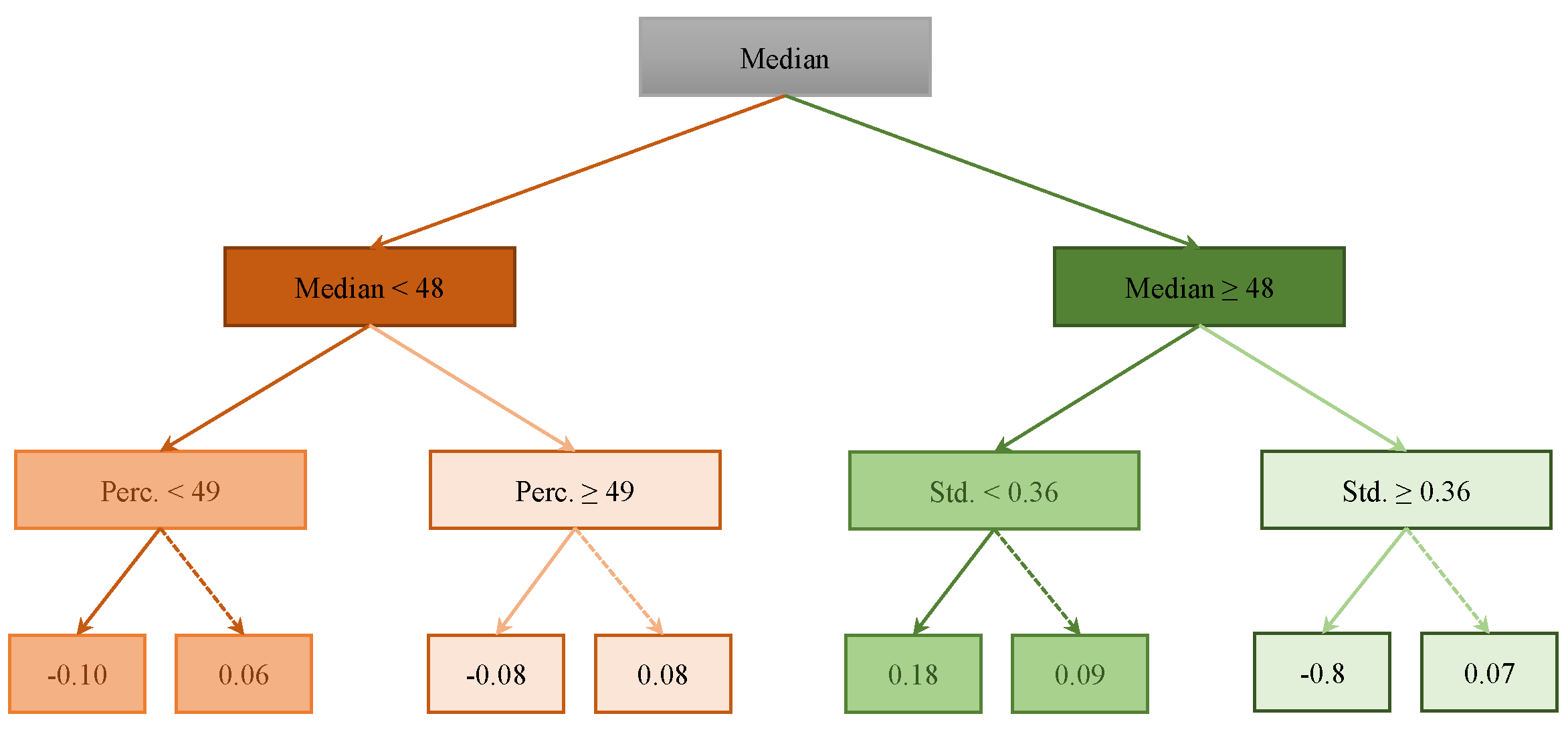
Figure 1. The architecture of gradient boosting machine. Rectangles in the figure show the split criteria while the end node is called ‘leaf’.
Applsci 10 02788 g001
Figure 2. The architecture of the support vector machines. The dashed lines on the figure shows the best dividing margins while the thick black line represent the dividing hyperplane as drawn by a support vector machine (SVM).
Applsci 10 02788 g002
Figure 3. Diagram for the proposed methodology. Initially pre-processing is carried out to remove noise and unnecessary data. Term Frequency-Inverse Document Frequency (TF-IDF) features are then extracted to train the classifiers. For evaluation train-test split is done as 70–30.
Applsci 10 02788 g003
Figure 4. Steps followed in the pre-processing of the data.
Applsci 10 02788 g004
Figure 5. Architecture of the proposed voting Classifier (GBSVM). ProbSVM-Pos represents SVM given probability score for a specific class while ProbGBM-Pos is for the GBM score of a particular class.
Applsci 10 02788 g005
Figure 6. Number of tweets in positive, negative and neutral classes.
Applsci 10 02788 g006
Table 1. Descripton of dataset attributes.
AttributeDescription
AppIt represent the actual name of the app on google play store.
Translated_ReviewsIt consists of the reviews given by each individual users.
SentimentsIt contains positive, Negative and Neutral sentiments.
Table 2. Parameters used for classifiers in experiments.
ParameterRFLRGBMSVMGBSVM
max_ depth10-10-10
learning_ rate--0.4-0.4
n_ estimators--100-100
random_ state21-2None2
C-1.0-1.01.0
cache_ size---200200
decision_ function_ shape---‘ovr’‘ovr’
degree---33
gamma---auto_ deprecated-
kernel---linearlinear
max_ iterations-100-−1−1
shrinking---TrueTrue
tol (tolerance)-0.0001-0.0010.001
penalty-L2---
fit_ intercept-True---
solver-lbfgs---
Table 3. Accuracy of classifiers using Term Frequency (TF) features.
ClassifierAccuracyNegative ClassNeutral ClassPositive Class
PrecisionRecallF1PrecisionRecallF1PrecisionRecallF1
GBSVM0.930.920.850.880.860.940.900.950.960.96
GBM0.910.910.800.850.780.950.860.950.950.95
SVM0.920.870.870.870.860.920.890.950.940.95
LR0.920.910.840.870.840.900.870.950.960.95
RF0.870.850.710.780.800.870.830.900.940.92
Table 4. Accuracy of classifiers using TF-IDF features.
ClassifierAccuracyNegative ClassNeutral ClassPositive Class
PrecisionRecallF1PrecisionRecallF1PrecisionRecallF1
GBSVM0.920.920.840.880.850.900.870.940.960.95
GBM0.910.920.820.870.800.940.860.950.950.95
SVM0.910.890.830.860.840.860.850.930.950.94
LR0.880.910.750.820.850.710.770.880.970.92
RF0.870.870.710.780.790.820.810.890.940.92
Table 5. Accuracy of classifiers using TF-IDF (Bi-gram) features.
ClassifierAccuracyNegative ClassNeutral ClassPositive Class
PrecisionRecallF1PrecisionRecallF1PrecisionRecallF1
GBSVM0.750.750.560.640.600.260.360.760.920.83
GBM0.700.760.360.490.460.180.260.710.940.81
SVM0.750.830.490.610.900.200.320.740.970.84
LR0.680.880.210.340.920.030.060.670.990.80
RF0.730.780.490.600.550.260.350.750.930.83
Table 6. Accuracy of classifiers using TF-IDF (Tri-gram) features.
ClassifierAccuracyNegative ClassNeutral ClassPositive Class
PrecisionRecallF1PrecisionRecallF1PrecisionRecallF1
GBSVM0.720.830.370.510.690.190.300.710.960.82
GBM0.680.840.180.300.770.110.190.670.990.80
SVM0.720.960.320.480.940.170.290.700.990.82
LR0.660.970.110.201.000.010.030.651.000.79
RF0.720.410.320.470.840.180.300.700.990.82
Table 7. Performance comparison of the proposed approach.
ApproachAccuracy
Reference [9] SGDC+LR88%
Reference [60] Rocchio+Naïve Byes+KNN73%
Proposed (GBSVM)93%
Table 8. Performance comparison of GBSVM against [62,63].
ApproachAccuracy
Reference [62] GCN87.9%
Reference [62] SGCN88.5%
Reference [63] NABoE86.0%
Proposed (GBSVM) with TF-IDF90.0%