Numerical and Experimental Analysis of Torsion Springs Using NURBS Curves

Abstract

Torsion springs, which transfer power through the twisting of their coil, provide advantages such as module simplification and efficient use of space. The design of a torsion spring has been formulated, but it is difficult to determine the local behaviors of torsion springs according to actual load conditions. This study proposes a torsion-spring design method through finite element analysis (FEA) using nonuniform-rational-basis-spline (NURBS) curves. Through experimentation, the angle and displacement values for the actual spring load were converted into useable data. Torsion-spring displacement values were obtained via experimentation and converted into coordinates that may be expressed using NURBS curves. The results of these experiments were then compared to those obtained via FEA, and the validity of this method was thereby verified.

1. Introduction

Torsion springs transfer power through the twisting of their coil, and provide advantages such as module simplification, efficient use of space, and reduction of overall product weight. As such, they have been widely used in various electronic products and industrial fields, including automobiles and machinery.

Research on these springs began in 1963 with Wahl’s study on isotropic spiral compression and tension, and torsion springs [1,2]. Thus far, the spring design formula proposed by Wahl is used as a standard and has been extensively employed in industrial-machinery applications. This applied design formula can easily calculate the rotation angle of the spring for the applied load. However, as this formula simplifies the problem, it is difficult to determine the behavior or deformation of a torsion spring according to the change in load conditions with different angles and directions.

Case studies considering the structural analysis of such springs using finite-element analysis (FEA) have been proposed to solve this design problem [3,4,5,6]. This method allows the designer to visually confirm and design these springs considering the stress and displacement that locally occur in the spring.

As FEA expresses curves as a sum of subdivided linear elements, many elements are needed to increase the reliability of curve-structure analysis. As springs are curved structures, the number of elements used in these analyses must inevitably be increased to ensure accuracy, thereby lengthening analysis time. Due to this increase in spring-design time, as well as the aforementioned design problem, and considering the effective product applications of these springs, a more effective torsion-spring design method is required.

This study proposes the evaluation method of deformation behavior of torsion spring via FEA using nonuniform-rational-basis-spline (NURBS) curves [7,8]. The NURBS curve is a model that can accurately express a curved structure with a small amount of information and a simple calculation formula. These curves were applied to FEA, and through experimentation, the angle and displacement values for the actual spring load were converted into useable data. The torsion-spring displacement values measured through experiments were converted into coordinates that could be expressed using NURBS curves. Experiments were then conducted for comparison with the FEA results and to verify the validity of this method.

2. Torsion-Spring Design

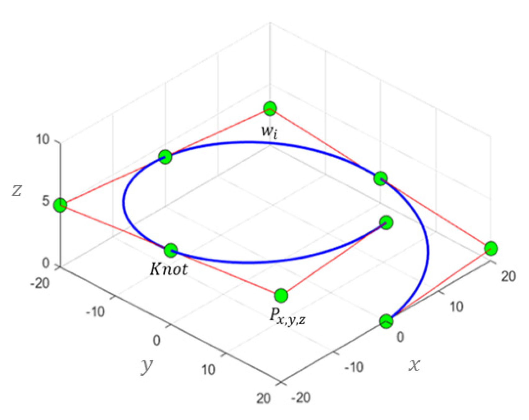
2.1. NURBS Curve

A range of research has been conducted on curve expression according to polynomial theory. Among the numerous curve-expression methods, NURBS is the most accurate technique used to express complex organic shapes in two and three dimensions [9,10]. Due to its simple calculation method, NURBS is employed in a variety of industrial fields that require curved shapes. A NURBS curve can be expressed through a combination of parameters, including knot, control point, degree, and weight, in basis functions with a relatively simple calculation algorithm. In NURBS curves, the initial basis function can be expressed as in Equation (1).

$$N\left(u\right)={{\displaystyle \sum }}_{i=0}^n{N}_{i,p}\left(u\right),$$

(1)

where $N_{i,p}\left(u\right)$ is the B-spline basis function. The equation applied to the algorithm differs with the number and value of the knot vectors; Equation (1) may also be expressed as either Equation (2) or Equation (3). To define B-spline basis functions, we need one more parameter: the degree of these basis functions, $p$. The i-th B-spline basis function of degree $p$, written as $N_{i,p}\left(u\right)$, is defined recursively as follows:

$$N_{i,0}\left(u\right)=\{\begin{array}{c}1 if u_i\le u\le u_{i+1}\\ 0, Otherwise\end{array}$$

(2)

$$N_{i,p}\left(u\right)=\frac{u-u_i}{u_{i+p}-u_i}{N}_{i,p-1\left(u\right)}+\frac{u_{i+p+1}-u}{u_{i+p+1}-u_{i+1}}{N}_{i+1,p-1}\left(u\right),$$

(3)

where $i$ is the degree plus 1 ($i=p+1$), $u_i$ is the knot, and $u$ is the knot vector. The following basis function expresses the curve of a geometric shape as the degree ($p$) increases; however, as the function increases in complexity and decreases in accuracy, a suitable degree should be used according to the desired curve shape. The NURBS basis function can express the NURBS curve as a combination of the weight ($w_i$) and control point ($P_i$), as shown in Equation (4).

$$C\left(u\right)={{\displaystyle \sum }}_{i=0}^n\frac{N_{i,p}{w}_i}{{{\displaystyle \sum }}_{j=0}^n{N}_{j,n}{w}_i}{P}_i=\frac{{{\displaystyle \sum }}_{j=0}^n{N}_{i,p}{w}_i{P}_i}{{{\displaystyle \sum }}_{j=0}^k{N}_{i,p}{w}_i},$$

(4)

where $P_i$ is the control point and $w_i$ is the weight of control point. This equation can then be simplified into Equation (5).

$$C\left(u\right)={\displaystyle \sum }_{i=0}^n{R}_{i,p}\left(u\right)P_i$$

(5)

The NURBS curve expressed by Equation (5) can be freely varied as the weight ($w_i$) increases and the control point ($P_i$)shifts, demonstrating the relationship between the NURBS curve and these parameters.

2.2. Expression of Torsion Spring Through NURBS Curves

To express the shape of a torsion spring with a constant curvature using the NURBS curve, Equations (6) to (8) are used for the x, y, and z planes on the global coordinate system.

$$x\left(u\right)={\displaystyle \sum }_{i=0}^n{R}_{i,p}\left(u\right)P_x$$

(6)

$$y\left(u\right)={\displaystyle \sum }_{i=0}^n{R}_{i,p}\left(u\right)P_y$$

(7)

$$z\left(u\right)={{\displaystyle \sum }}_{i=0}^n{R}_{i,p}\left(u\right)P_z,$$

(8)

where ${\mathit{P}}_{\mathit{N}}$ are the coordinates of the interpolation point generated through the initial NURBS curve, and ${\mathit{P}}_{\mathit{N}\mathit{d}\mathit{i}\mathit{s}\mathit{p}}$ are the coordinates through a combination of the knot, control point, and weight (Equations (6) to (8)). The spring shape can be expressed on three planes in 3D space, as shown in Figure 1.

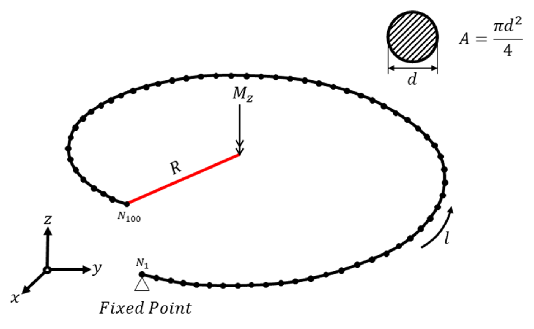
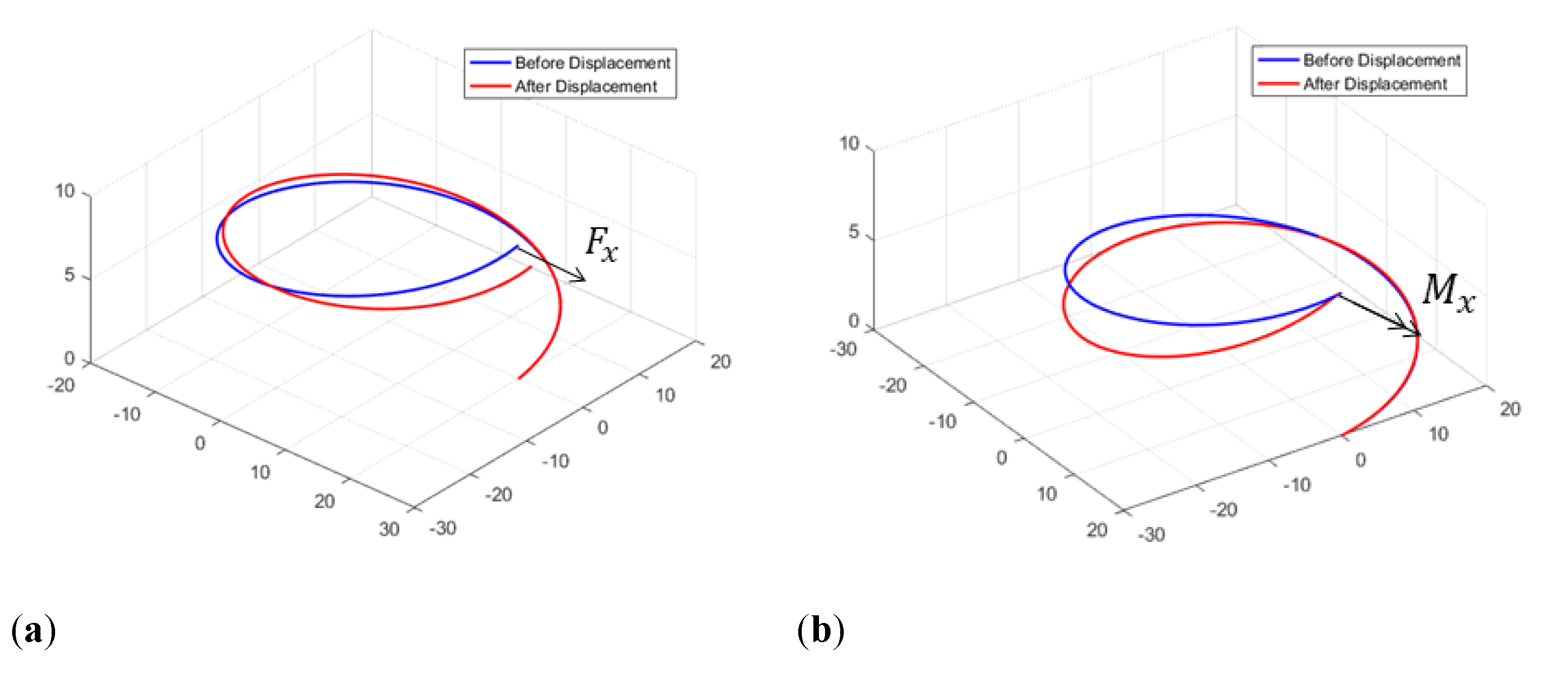
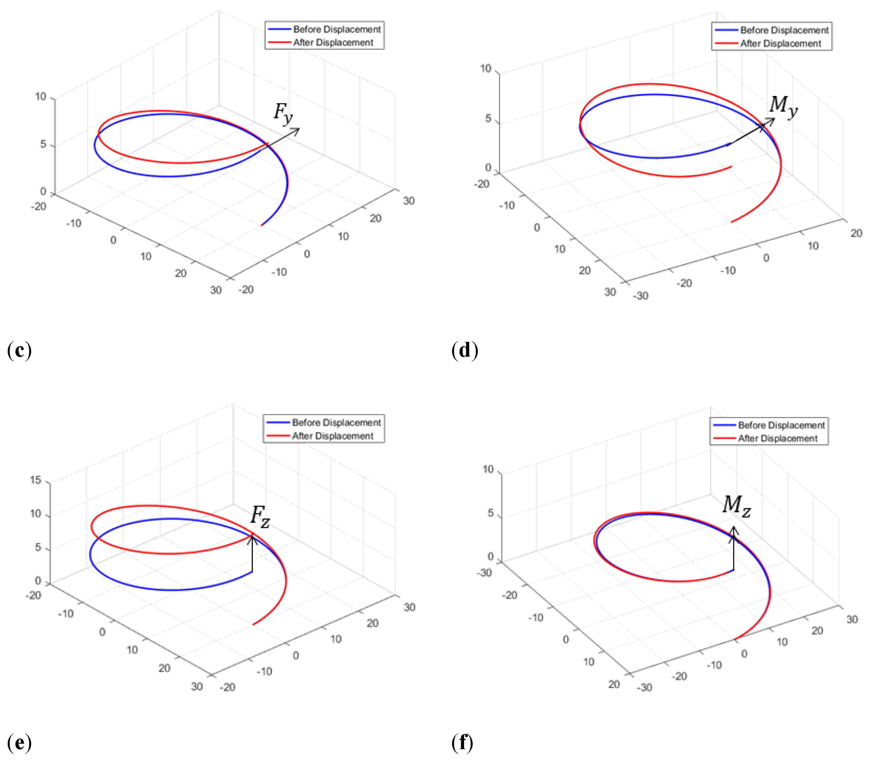
3. Torsion-Spring Displacement Analysis

3.1. Torsion-Spring Displacement Analysis

To verify the correlation between the interpolation point and control point, the coordinates of the interpolation point generated through the NURBS curve are applied to finite-element analysis to create the torsion-spring shape for analysis [11,12,13]. Figure 2 shows the finite-element model of the torsion spring that was used to derive the displacement of the control point as it shifted according to the external force [14,15].

Table 1. Design parameters.

Parameters	Unit	Dimension
Spring cross-section diameter ($d$)	mm	3
Spring radius ($R$)	mm	20
Spring length ($\mathit{l}$)	mm	125.6
Moment in the z-axis direction (${\mathit{M}}_{\mathit{z}}$)	N m	1000
Elastic modulus	GPa	206

shows the parameters of the model used for analysis. Commercial software HyperWorks Optistruct (Altair, United States) was used for finite-element analysis, and the shifted displacement data were acquired for generated moment $M_z$. The displacement values shifted after the generation of the initial coordinates, and loads were analyzed for a total of 100 elements ($N_i$).

The displacement of the element determined through finite-element analysis (${\mathit{x}}_{\mathit{d}\mathit{i}\mathit{s}\mathit{p}}$, ${\mathbf{y}}_{\mathbf{d}\mathbf{i}\mathbf{s}\mathbf{p}}$, ${\mathbf{z}}_{\mathbf{d}\mathbf{i}\mathbf{s}\mathbf{p}}$) was added to the coordinates of the interpolation point generated through the NURBS curve to express the deformed shape of the spring. This is expressed using Equations (9) to (11).

$$P_{Ndisp}\left(x\right)=P_N\left(x\right)+x_{disp}$$

(9)

$$P_{Ndisp}\left(y\right)=P_N\left(y\right)+y_{disp}$$

(10)

$$P_{Ndisp}\left(z\right)=P_N\left(z\right)+z_{disp}$$

(11)

where $P_N$ are the coordinates of the interpolation point generated through the initial NURBS curve, and $P_{Ndisp}$ are the coordinates of the interpolation point of the NURBS curve after deformation.

The coordinates of $P_{Ndisp}\left(x, y,z\right)$, derived from Equations (9) to (11), were next applied to the inverse method to determine the displacement of the control point. This process is shown in Equation (12), which was derived with reference to Equations (4) and (5). Figure 3 shows the control point derived using Equation (12),

$$P_{\left(x,y,z\right)}=\frac{{{\displaystyle \sum }}_{i=1}^n{R}_{i,p}\left(u\right)}{P_{Ndisp}\left(x,y,z\right)},$$

(12)

where $P_x$, $P_y$ and $P_z$ are the coordinates of the control point, and $R_{i,P}\left(u\right)$ is the NURBS curve-based function.

In Figure 3,${\left(x,y,z\right)}_{disp}$ represents the x, y, and z displacements of the point; $P_N\left(x,y,z\right)$ represents the coordinates of the point before interpolation; and $P_{Ndisp}\left(x,y,z\right)$ represents the coordinates of the point after interpolation. The inverse method can be applied to determine the displacement and load as $K_{NURBS}$.

$$a\left[D\right]=a{\left[K\right]}^{-1}\left[F\right],$$

(13)

where $\left[D\right]$ is the displacement matrix of the control point derived from the existing stiffness matrix,$a$ is the stiffness-correction constant,${\left[K\right]}^{-1}$ is the inverse of the stiffness matrix, and $\left[F\right]$ is the external force matrix. Stiffness-correction constant $\mathrm{a}$ can be expressed as follows:

$$a={\left[a_i\right]}^T.$$

(14)

Thus, the following is obtained by applying Equation (14) to Equation (13).

$${\left[a_i\right]}^T\left[D\right]={\left[a_i\right]}^T{\left[K\right]}^{-1}\left[F\right]$$

(15)

Equation (15) can then be expressed as in Equation (16).

$$\left[D_{\in v}\right]={\left[K_{NRBS}\right]}^{-1}\left[F\right]$$

(16)

where $\left[D_{\in v}\right]$ is the control point displacement determined using the inverse method, and ${\left[K_{NRBS}\right]}^{-1}$ is the inverse of the stiffness matrix of the control point.

Using Equation (16), the $M_z$ load was applied to the NURBS curve-based spring structure that was composed of a total of nine control points, and analysis was conducted.

Using this method, the graphs in Figure 4 were derived for loads $F_x$, $F_y$, $F_z$, $M_x$, $M_y$, and $M_z$.

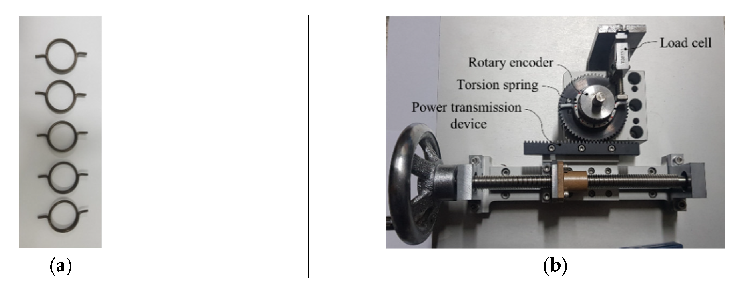
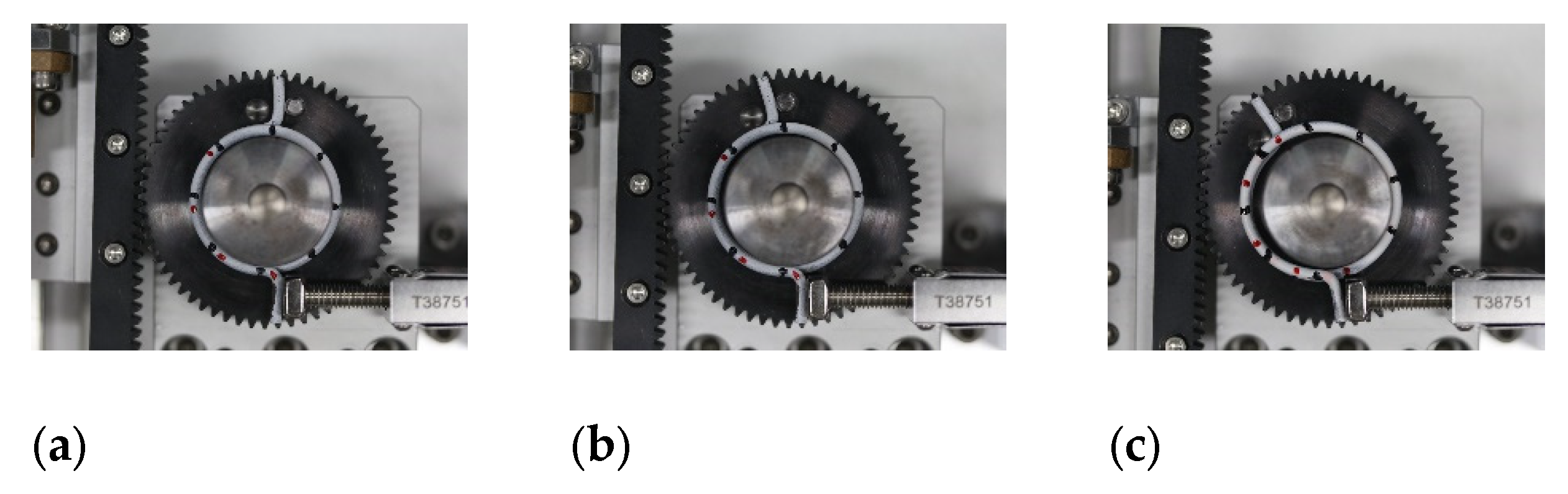
3.2. Experiment-Equipment Setup

Experiments were conducted to measure the displacement, load, and angle using a torsion-spring measuring device. Torsion-spring parameters were selected for a total of six types of specimens. Five experiments were conducted for each specimen, resulting in a total of 30 experiments.

Table 2. Specimen types.

Type	$\mathbf{Spring}\mathbf{Cross}-\mathbf{Sec}\mathbf{tion}\mathbf{Diameter},\mathbf{d}$ (mm)	$\mathbf{Spring}\mathbf{Diameter},\mathbf{D}$ (mm)	$\mathbf{Spring}\mathbf{Turns},\mathit{N}$
1	2.6	32.6	1.5
2	2.6	32.6	2.5
3	2.8	32.8	1.5
4	2.8	32.8	2.5
5	3.0	33.0	1.5
6	2.0	33.0	2.5

shows the design parameters of the six spring specimens. The experiment equipment was configured to measure the torsion spring. Figure 5 shows the actual torsion spring and the device used to measure the spring displacement, load, and angle. The rotation angle was set to 0°, 20°, and 40°, considering the linear component of the load applied to the torsion spring. To determine torsion-spring displacement, certain sections were marked, and displacement and load values were measured at 20° and 40°. Images were taken of the front of the system to determine the x and y coordinates, and the z-axis was measured through images of the sides and Vernier calipers.

4. Results and Discussion

4.1. Experiment-Data Analysis

The force according to the rotation angle was measured using a load cell and rotary encoder. Figure 6 shows images of the x- and y-coordinate measurements obtained according to the angle of the torsion spring, and Figure 7 shows a load graph according to the rotation angle. This graph was drawn using the average data from the results of five replicates. Analytical results indicated that the torsion-spring load was generated nonlinearly according to the rotation angle. The regression equation was derived using the measured data and was expressed as a quadratic polynomial in the graph. R-square values of the regression equations were 98% or more. This regression equation had a high adjustment. In addition, it was found that the load increased as the cross-sectional diameter ($\mathrm{d}$) of the torsion spring increased, and that the load decreased as the number of spring turns ($N$) increased.

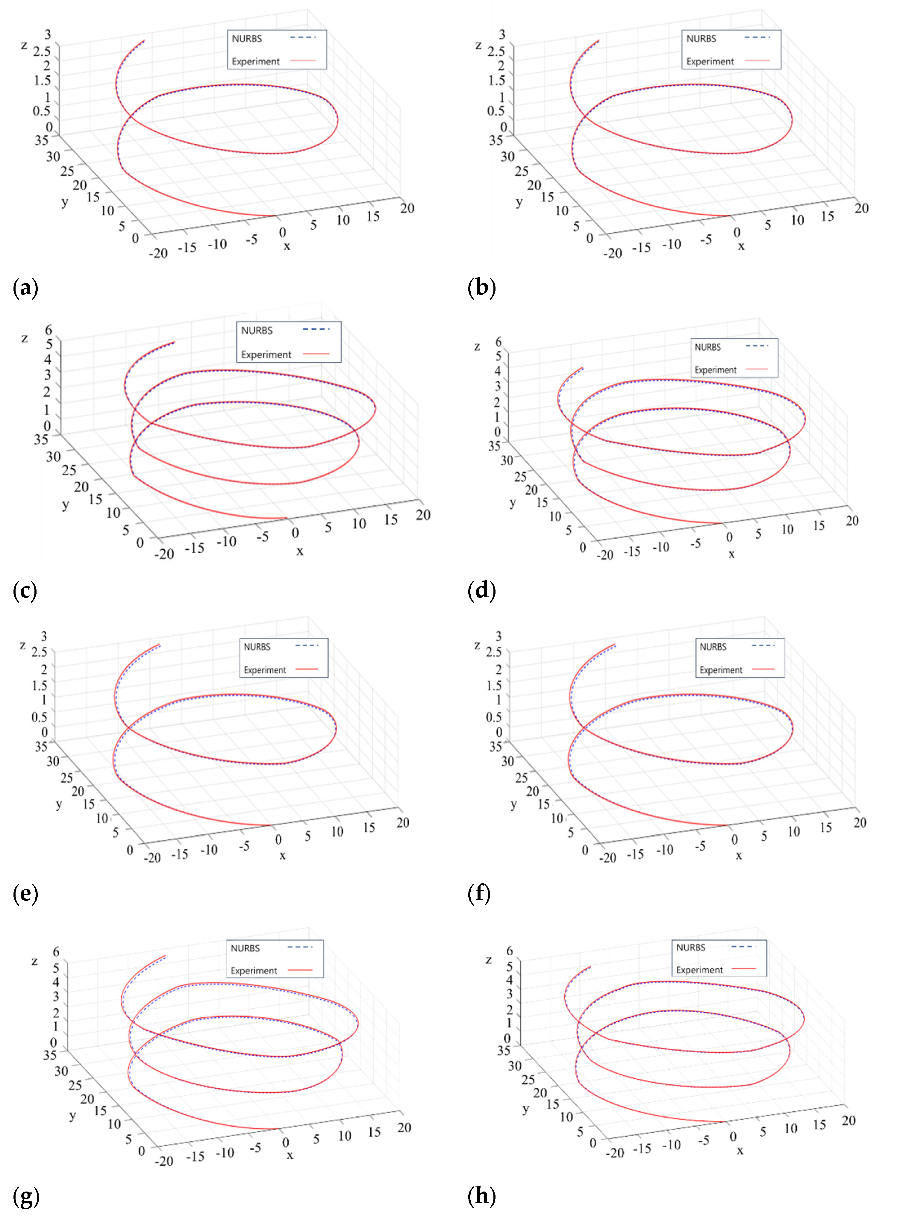
4.2. Comparative Analysis of Analytical Results and Experiment Values

We performed comparative analysis of the deformed shape of the torsion spring, measured through the experiments, and the analytical results obtained using Equation (16). Figure 8 shows graphs of the analytically and experimentally obtained data. We then performed comparative analysis of the deformed shape of the torsion spring at 20° and 40°, measured through the experiments and Equation (16). Under the same load conditions, the displacement determined by the proposed equation exceeded that of the torsion spring measured through the experiments. However, by modifying the load parameters, similar behaviors and displacements were observed, thereby verifying the use of the proposed equation. The maximal error rate ranged from 5% to 6%, which could be attributed to the error that can occur during experiment measurements.

5. Conclusions

This study applied nonuniform-rational-basis-spline (NURBS) curves for the design of torsion springs, analyzed the displacements of these springs using finite-element analysis, and verified the design of these springs through experimentation.

(1) A method was proposed for deriving the coordinates of a control point for shifted elements by applying the inverse method on the basis of data derived through finite-element analysis. In addition, the relationship between the movement of the control point and stiffness matrix was identified and formulated by varying the torsion-spring parameters.

(2) A method was proposed for deriving the torsion-spring shape by converting the torsion-spring displacement measured through experiments into coordinates that could be expressed using NURBS curves.

(3) Comparative analyses between the results of the proposed analytical method and the experiment measurements demonstrated that the proposed method is valid within a satisfactory range of error.

References

1. Yuldirim, V. Exact determination of the global tip deflection of both close-coiled and open-coiled cylindrical helical compression spring having arbitrary doubly-symmetric cross-section. Int. J. Mech. Sci. 2016, 115–116, 280–298. [Google Scholar] [CrossRef]
2. Wahl, A.M.; Bisshopp, K.E. Mechanical Springs (Second Edition). J. Appl. Mech. 1964, 31, 159–160. [Google Scholar] [CrossRef]
3. Pollanen, I.; Martikka, H. Opimal re-design of helical spring using fuzzy design and FEM. Adv. Eng. Softw. 2010, 41, 410–414. [Google Scholar] [CrossRef]
4. Chaudhury, A.N.; Datta, D. Analysis of prismatic springs of non-circular coil shape and non-prismatic springs of circular coil shape by analytical and finite element methods. J. Comput. Des. Eng. 2017, 4, 178–191. [Google Scholar] [CrossRef]
5. Gzal, M.; Groper, M.; Gendelman, O. Analytical, experimental and finite element analysis of elliptical cross-section helical spring with small helix angle under static load. Int. J. Mech. Sci. 2017, 130, 476–486. [Google Scholar] [CrossRef]
6. Chassie, G.; Becker, L.; Cleghorn, W. On the buckling of helical springs under combined compression and torsion. Int. J. Mech. Sci. 1997, 39, 697–704. [Google Scholar] [CrossRef]
7. Gao, J.; Luo, Z.; Xiao, M.; Gao, L.; Li, P. A NURBS-based Multi-Material Interpolation (N-MMI) for isogeometric topology optimization of structures. Appl. Math. Model. 2020, 81, 818–843. [Google Scholar] [CrossRef]
8. Alderson, T.; Samavati, F. Multiscale NURBS curves on the sphere and ellipsoid. Comput. Graph. 2019, 82, 243–249. [Google Scholar] [CrossRef]
9. Timoshenko, S.P. Mechanics of Materials; Chaoman & Hall: London, UK, 1911. [Google Scholar]
10. Piegl, L.; Tiller, W.; Piegl, L. The NURBS Book; Springer: Heidelberg, Germany, 1997. [Google Scholar]
11. Ferreira, A.J.M. MATLAB Codes for Finite Element Analysis: Solid Mechanics and its Applications; Springer: Heidelberg, Germany, 2008; Volume 157. [Google Scholar]
12. Shimoseki, M.; Hamano, T.; Inaizumi, T. FEM for Springs; Springer Science & Business Media: Berlin, Germany, 2013. [Google Scholar]
13. Zhao, X.-Y.; Zhu, C. Injectivity of NURBS curves. J. Comput. Appl. Math. 2016, 302, 129–138. [Google Scholar] [CrossRef]
14. Zhang, B.; Li, C.; Wang, T.; Wang, Z.; Ma, H. Design and experimental study of zero-compensation steering gear load simulator with double torsion springs. Meas. 2019, 148, 106930. [Google Scholar] [CrossRef]
15. Kilic, M.; Yazicioglu, Y.; Kurtulus, D.F. Synthesis of a torsional spring mechanism with mechanically adjustable stiffness using wrapping cams. Mech. Mach. Theory 2012, 57, 27–39. [Google Scholar] [CrossRef]
Figure 1. Representation of nonuniform-rational-basis-spline (NURBS) curves coupled in 3D space.
Applsci 10 02629 g001
Figure 2. Finite-element model of torsion spring.
Applsci 10 02629 g002
Figure 3. Derivation of control point using inverse method.
Applsci 10 02629 g003
Figure 4. Direction-displacement graphs for load conditions (a) F x , (b) M x , (c) F y , (d) M y , (e) F z , (f) and M z .
Applsci 10 02629 g004aApplsci 10 02629 g004b
Figure 5. Springs and experiment setup: (a) torsion springs; (b) experiment setup.
Applsci 10 02629 g005
Figure 6. Measurement of x- and y-coordinates of torsion springs: (a) 0°; (b) 20°; (c) 40°.
Applsci 10 02629 g006
Figure 7. Force vs. degree graph of torsion springs.
Applsci 10 02629 g007
Figure 8. Comparative analysis of torsion springs: (a) d = 2.6 mm, D = 32.6 mm, n = 1.5 (20°); (b) d = 2.6 mm, D = 32.6 mm, n = 1.5 (40°); (c) d = 2.6 mm, D = 32.6 mm, n = 2.5 (20°); (d) d = 2.6 mm, D = 32.6 mm, n = 2.5 (40°); (e) d = 2.8 mm, D = 32.8 mm, n = 1.5 (20°); (f) d = 2.8 mm, D = 32.8 mm, n = 1.5 (40°); (g) d = 2.8 mm, D = 32.8 mm, n = 2.5 (20°); (h) d = 2.8 mm, D = 32.8 mm, n = 2.5 (40°); (i) d = 3.0 mm, D = 33.0 mm, n = 1.5 (20°); (j) d = 3.0 mm, D = 33.0 mm, n = 1.5 (40°); (k) d = 3.0 mm, D = 33.0 mm, n = 2.5 (20°); (l) d = 3.0 mm, D = 33.0 mm, n = 2.5 (40°).
Applsci 10 02629 g008aApplsci 10 02629 g008b