Article

A Steering-Following Dynamic Model with Driver’s NMS Characteristic for Human-Vehicle Shared Control

1
School of Mechatronics & Vehicle Engineering, Chongqing Jiaotong University, Chongqing 400000, China
2
Chongqing Key Laboratory of “Human-Vehicle-Road” Cooperation & Safety for Mountain Complex Environment, Chongqing Jiaotong University, Chongqing 400000, China
*
Author to whom correspondence should be addressed.
Appl. Sci. 2020, 10(7), 2626; https://doi.org/10.3390/app10072626
Submission received: 6 February 2020 / Revised: 6 April 2020 / Accepted: 8 April 2020 / Published: 10 April 2020
(This article belongs to the Special Issue Artificial Intelligence for Connected and Automated Vehicles)

Abstract

:
For investigating driver characteristic as well as control authority allocation during the process of human–vehicle shared control (HVSC) for an autonomous vehicle (AV), a HVSC dynamic mode with a driver’s neuromuscular (NMS) state parameters was proposed in this paper. It takes into account the driver’s NMS characteristics such as stretch reflection and reflex stiffness. By designing a model predictive control (MPC) controller, the vehicle’s state feedback and driver’s state are incorporated to construct the HVSC dynamic model. For the validation of the model, a field experiment was conducted. The vehicle state signals are collected by V-BOX, and the driver’s state signals are obtained with the electromyography instrument. Subsequently, the hierarchical least square (HLS) parameter identification algorithm was implemented to identify the parameters of the model based on the experimental results. Moreover, the Unscented Kalman Filter (UKF) was utilized to estimate the important NMS parameters which cannot be measured directly. The experimental results showed that the model we proposed has excellent accuracy in characterizing the vehicle’s dynamic state and estimating the driver’s NMS parameter. This paper will serve as a theoretical basis for the new control strategy allocation between human and vehicle for L3 class AVs.

1. Introduction

Significant progress has been conducted in the field of perception, decision making, path planning and control authority for autonomous vehicles (AVs) in the past few decades. However, it is still far away from widespread market penetration because of its unmatured technology. As a promising technique aimed at improving the safety of AV, the concept of “human–vehicle shared control” (HVSC) has achieved a great deal of research effort in recent years [1]. For HVSC, the automation and driver take control authority of the vehicle sequentially after each other, or co-pilot the vehicle simultaneously [2].
The dynamic model is of great significance for the understanding of the intrinsic and developing control authority of HVSC. In this way, many existing scholarly works have demonstrated the contributions associated with the dynamic model in the HVSC domain. For example, the biomechanical properties of the driver for a vehicle steering task is considered a novel technique of estimating the admittance and total response [3]. By investigating the influence of haptic aids on the pilot’s NMS response, an online estimator of the time-varying NMS dynamic method based on Recursive Least Squares is proposed [4,5]. On the basis of the electric power-assisted steering system, Marouf A et al. [6] proposed a time-varying method based on a sliding mode observer and the exponentially weighted recursive least squares (EWRLS) algorithm for the estimation of the viscoelastic properties in the driver’s arm. The characterization of driver NMS dynamics, implemented to analyze the influence of active and passive steering tasks and hand positions, is also highly sought after [7]. Subsequently, in order to further reflect the relationship between driver and vehicle, the novel Queuing Network is integrated into the driver’s NMS dynamic [8]. Similarly, by reducing the internal cost function of the driver, a human–vehicle steering control strategy with the driver’s NMS dynamic is proposed [9]. In this way, an intra-driver variability human-like steering model inspired the research boom [10]. Soon after, Yanbo Z et al. [11] proposed a shared steering controller by imitating the driver’s characteristics of the NMS system. Furthermore, other physiological characteristics including the driver’s vision and blood volume pulse, which are regarded as vital indexes, are utilized to demonstrate the mechanism of driving behavior and construct the human–vehicle shared control model [12,13].
When the driver executes the operation of following the leading car, the driver’s leg model plays a vital role in HVSC. In regard to this field, the pedal drive unit is applied to the human–machine interface analysis experiment by investigating the physiological characteristics of the driver’s leg [14]. It is noteworthy that the mechanism of the individual muscle-tendon biomechanics metabolism also is parsed, and then a Hill-based human leg model with a muscle and joint is proposed [15]. In further research, a put-forward two-dimensional leg model with a knee, along with ankle passive and quasi-passive elements is optimized [16]. By investigating the influence of muscle force during flexion–extension movement, a Hill-based electromyography (EMG)-driven model of the elbow is proposed [17].
In light of our literature review, there are only a few studies involved in the following aspects. The current driver dynamic models with NMS characteristic are only represented by a single steering arm. The leg NMS dynamic of the driver was not taken into account thoroughly. Particularly in the condition of a roundabout or overtaking, the driver executes the sequential steering–following operation. Therefore, the relative influence between arm and leg NMS characteristic should not be neglected for practical application of the dynamic model. For L3 autonomous vehicle (AV), the driver is required to take over the control authority of the vehicle when the automation system fails to deal with the emergency situation. Most of time, the driver will be disengaged from the human–vehicle–road closed loop. Therefore, frequently, discrete interactions between the driver and vehicle will cause the degradation of the human’s cognitive ability and driving skills. Consequently, it will affect the driver’s NMS dynamic properties, such as viscoelastic resistance coefficient and movement feedback coefficient. Moreover, the driver’s NMS model was not analyzed by employing the EMG signals of the driver for validation.
In this paper, a HVSC dynamic model incorporating the arm and leg NMS characteristics of the driver is proposed. The EMG signals are collected and then muscle force is decomposed based on the Hill muscle contraction theory. The hierarchical least square method is applied to identify the off-line parameters of the dynamic model. Thereafter, the Unscented Kalman Filter (UKF) observer is designed to estimate the NMS characteristic parameters. The structure of the article is organized as follows: Section 2 illustrates the schematic of HVSC model. Section 3 describes the scenario and the procedure of the field experiment. The offline identification of the model’s parameter and online estimation by means of UKF observer are demonstrated in Section 4. The proposed dynamic model is validated using experimental results in Section 5. A brief summary and discussion are present in the last section.

2. Materials and Methods

By designing a model predictive control (MPC) controller with vehicle’s state feedback, a HVSC dynamic model is constructed in this paper. Specifically, the function of the MPC controller is to keep tracking the trajectory to generate the anticipated steering wheel angle δ ^ s w and gas pedal position θ ^ p e d . After receiving the anticipated angle δ ^ s w , the driver’s NMS model produces the actual steering angle δ s w and gas pedal position θ p e d ( f ) signal feedback to controller backward. The NMS dynamic model of the driver is composed of 11 components. The schematic of the HVSC dynamic model is illustrated as Figure 1.

2.1. Subsection

The dynamic response of the driver’s arms applied at the steering wheel can be represented by a parallel spring and damper, as shown in Table 1. The passive damping and stiffness of the arms represent the properties of the muscles, skin and tendons in relaxation, which can be simplified as arm inertia J d r , arm damping B d r and arm stiffness K d r systems [18]. The steering system, including the steering wheel, column, rack and pinion, uprights and wheels and tires can also be represented as simple inertia J s t , damper B s t and spring K s t systems. In addition, the torque feedback term K a is inferred to the torque M t obtained from the slip angle at the front axle [19].
The steering mechanism dynamics and steering arm dynamics are coupled at the point where the driver grips the steering wheel. The equation of motion and corresponding transfer function is obtained as follows:
( J d r + J s t ) δ ¨ sw + ( B d r + B s t ) δ ˙ sw + ( K d r + K s t ) δ sw = T m M T n r s w
G s ( s ) = 1 / [ ( J d r + J s t ) s 2 + ( B d r + B s t ) s + ( K d r + K s t ) ]
where T m represents the total muscle torque applied at the steering wheel; n r s w and δ sw indicate the steering gear ratio and wheel steering angle respectively.
The spindle feedback muscle information is transferred to the alpha-motor neurons to maintain muscle length. The reflex control of muscle length can cause a change in the intrinsic passive stiffness and damping of the muscle. The value of the reflex gain varies depending on muscle activation [20]. The reflex control dynamic can be expressed as Equation (3):
H r ( s ) = [ ω c ( s B r + K r ) e s τ d e l ] / ( s + ω c )
where ω c refers to the cutoff frequency; B r indicates the reflection damping.
Noteworthily, the inherent time delay can be approximated as a first-order transfer function:
e s τ d e l 1 / ( 1 + τ d e l s )
The steering torque command is generated by a reference model, which is, essentially, a learned inverse model of the arms, steering and vehicle. The following reference model dynamic is extremely appropriate for real driver behavior [20].
G ^ ( s ) = 0.067 0.028 s 2 + 0.083 s + 1

2.2. Leg NMS Dynamic Model

The admittance H a d m can be parameterized by a linear NMS model which represents the dynamics of the ankle–foot interaction with the gas pedal in Figure 1. The inputs of the NMS model are the disturbing torque T d i s and the anticipated gas pedal position θ ^ p e d . The measurable model outputs are T c and θ c [21]. The model structure is an extension of NMS models proposed in previous research [22].
The inertia component can be described by the endpoint inertia of the limb I s e g in the form of a transfer function as follows:
H s e g ( s ) = 1 I s e g s 2
The muscle contact dynamic is described as:
H c ( s ) = k c o n + b c o n s
The intrinsic component is defined by the activated muscle stiffness k int and damping b int in the form of transfer function:
H int ( s ) = k int + b int s
The reflexive component can be deduced as follows:
H a c t ( s ) = 1 ( 1 ω 0 2 ) s 2 + 2 β ω 0 s + 1
The muscle golgi tendon organs (GTO) dynamic can be demonstrated as:
H g o t ( s ) = k f e τ d e l s
The muscle spindle dynamic is expressed as:
H m s ( s ) = ( K p o s + K v e l s ) e s · τ d e l
where the K p o s and K v e l represent the gains of the monosynaptic stretch and stretch velocity feedback respectively.
As a serial elastic element to the muscles, tendons dynamic can be expressed as:
H t e n d ( s ) = 1 k t e n d
where k t e n d represents the stiffness of the tendon.
Noteworthily, the motion of the inertia I s e g is the result of the sum of T c ( s ) and T m u s ( s ) . The pedal–torque can be combined with the muscles, partially. Then, the motion of the limb is deduced as:
θ lim b ( s ) = H s e g ( s ) [ T c ( s ) + T m u s ( s ) ]
Pedal rotations do not only cause joint rotations but also small displacements of the skin or soft tissue. This effect is described by contact dynamics as follows:
T c ( s ) = H c ( s ) [ θ c ( s ) θ lim b ( s ) ]

2.3. Vehicle Dynamic Model

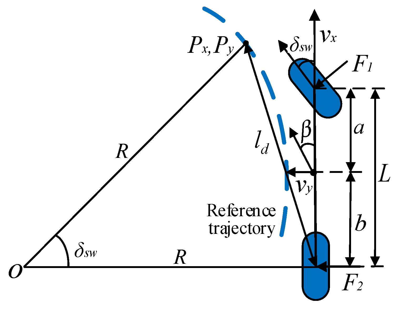
During the process of HVSC, the lateral and yaw motion of the vehicle are critical issues. A simplified linear two-degree-of-freedom (2DOF) lateral dynamic model is widely utilized to investigate the characteristic of human–automation interaction [23]. The geometric relationship and parameters of the vehicle dynamic model are listed in Figure 2 and Table 2:
The equations of the lateral and yaw moment are denoted as:
{ v ˙ y = ( k 1 + k 2 ) m v x v y ( v x ( b c r a c f ) m v x ) ω r + k 1 m δ s w ω ˙ r = ( b k 2 a k 1 ) I z v x v y ( b 2 c r + a 2 c f ) I z v x ω r + a k 1 I z δ s w
where vy represents lateral speed; ωr infers to yaw rate. The lateral offset ey is described as:
e ˙ y = v y + x l ω r + v x ψ
where ψ represents the yaw angle.

2.4. MPC Controller

In order to incorporate the vehicle dynamics with road trajectory, a great deal of investigation of trajectory tracking was conducted. Inspired by appropriate literature, the MPC controller is implemented in this section for strong robustness and stability in trajectory tracking [24]. The main steps of the MPC controller are given in Algorithm 1:
Algorithm 1. MPC controller.
Input_U: {Vehicle state variable V c u r ; Road trajectory}
Step1: Construct vehicle predictive model:
ξ ( k | t ) = [ V ( k | t ) u ( k 1 | t ) ]
{ ξ ( k + 1 | t ) = A k , t ξ ( k | t ) + B k , t Δ U ( k | t ) V ( k | t ) = C k , t ξ ( k | t )
y ( t ) = Ψ t ξ ( t | t ) + Θ t Δ U ( t )
Step2: Calculate cost function:
J ( t ) = i = 1 N p V ( t + i | t ) V r e f ( t + i | t ) Q 2 + i = 1 N c 1 u ( t + i | t ) R 2 + ρ ε 2
Step3: Set constraints:
Δ U min Δ U t Δ U max
U min A Δ U t + U t U max
y h c , min y h c y h c , max
y s c , min ε y s c y s c , max + ε
ε > 0
Output_y: {Anticipated steering wheel angle δ ^ s w ; Anticipated pedal position θ ^ p e d }

2.5. Model Integration

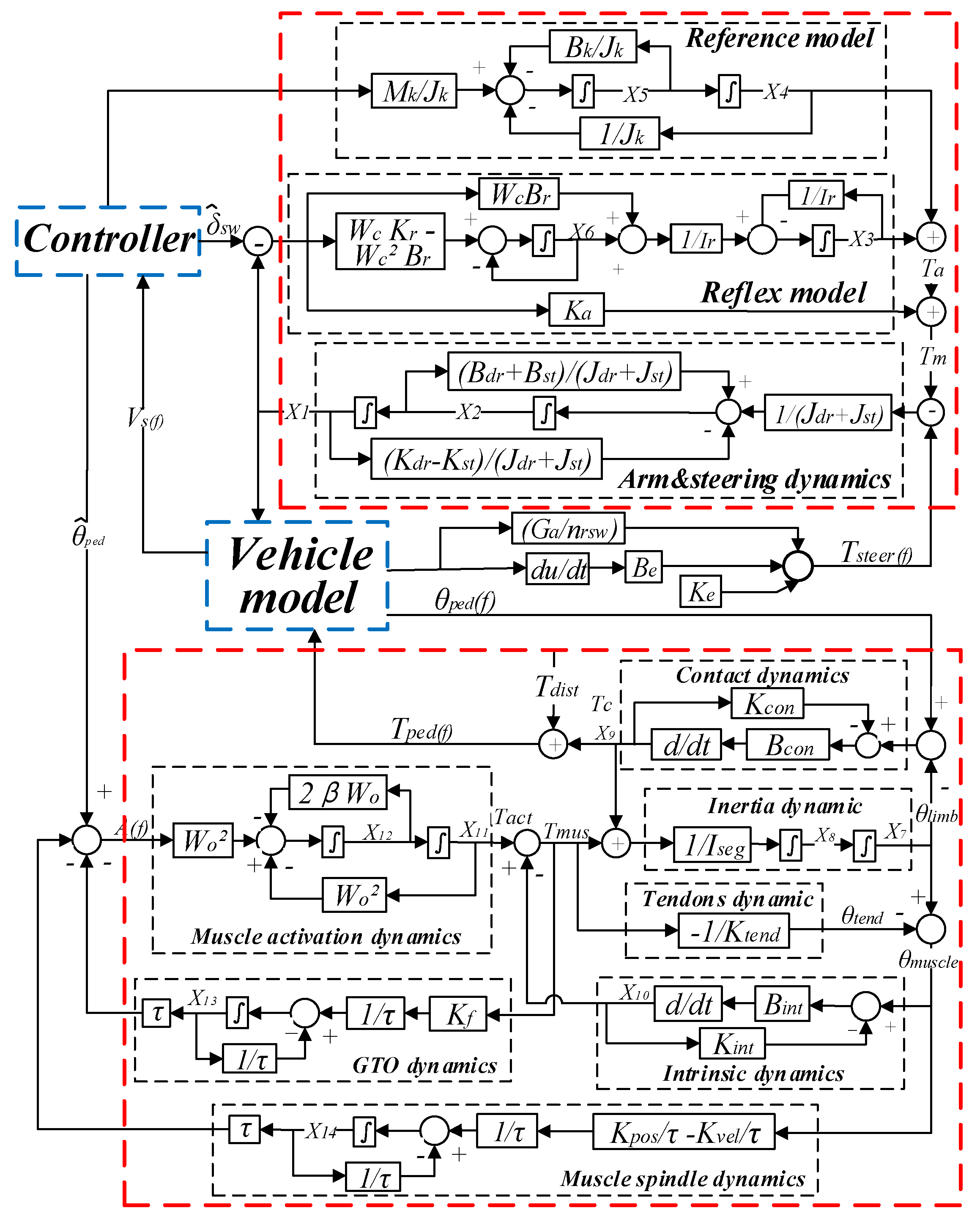
Considering that the vehicle dynamic model is constructed in the form of state-space equation, the driver’s NMS dynamic expressed as transfer functions should be converted to the state equation. From the aspect of theoretic analysis, the n-order transfer function can be decomposed into the product of several one-order transfer functions. Then the system state variable diagram is formed in series by one-order transfer functions [25]. In this way, the HVSC state equation form the block diagram can be constructed as shown in Figure 3.
A total of 17 state variables are defined in Figure 3.The physical sense of δ sw , δ ˙ s w , T a c a , T ξ c , T r c , T c c a , θ lim b , θ lim b , T c c l , T int , T a c l , T a c l , T g o t and T s p represents the steering wheel angle, steering wheel angular rate, arm active contraction torque, reference contraction torque, contact contraction torque, reflex contraction torque, leg motion, leg motion rate, leg contact contraction torque, leg intrinsic contraction torque, leg active contraction torque, leg active reference torque, leg GTO feedback torque and leg spindle feedback torque respectively. Noteworthily, the physical value of some state variables cannot be obtained directly from the sensor. Therefore, a state observer based on UKF is proposed to estimate these variables. The relationship between state variables and measurable variables was elaborated on in the following content [26].
First, the muscle contraction force F i is deduced based on Hill muscle theory as follows:
F i = F ce + F pe = F max [ a ( i ) f a ( ε ) + f p ( ε ) ] = F max [ a ( i ) e [ 2.7272778 × ln ( ε + 1 ) ] 2 + 0.03 ( e 7 ε 1 ) ]
where Fce represents muscle contraction force; Fpe infers to the elastic force; F max indicates the muscle maximum contraction force; a ( i ) is the muscle activation; f a ( ε ) and f p ( ε ) infer to the active and passive contraction of the muscle; ε represents deformation degree of the muscle during contraction.
Afterward, the weighted analysis method is used to calculate the arm active contraction torque T a c a and leg active contraction torque T a c l applied to the steering wheel and pedal respectively as follows:
{ T a c a = ( F 1 n 1 + F 2 n 2 + + F i n i ) / R a ; i = 6 T a c l = ( F 1 n 1 + F 2 n 2 + + F i n i ) / R l ; i = 4
where n i infers to the weight coefficient of muscle force; Ra and Rl represent the radius of the steering wheel and pedal rotation.
For the arm dynamic model, the arm reflex contraction torque T r c can be deduced based on T a c a and assist torque T a s applied on the steering wheel, which can be express as Equation (19):
T r c = T a c a T a s
The arm reference contraction torque T ξ c and arm contact contraction torque T c c a can be described as follows:
T ξ c + T c c a + K a ( θ s w θ ^ s w ) = T d r
T c c a = T s w T d i s
where K a represents the active stiffness; T d r infers to the steering wheel torque; T s w infers to the torque applied on the steering wheel; T d r indicates the steering torque of vehicle; T d i s is the torque perturbation from the sensor.
As shown in Figure 3, the feedback torque T f e e d can be calculated as steering angle feedback and acquired steering angle, denoted as Equation (22)
T f e e d = δ sw K e + δ sw · B e + G a / n r s w
where T f e e d is the steering wheel torque feedback; K e is the gain coefficient of steering angle; B e represents the gain coefficient of steering speed; G e represents the kingpin caster angle gain coefficient.
For the leg dynamic model, the leg contact contraction torque T c c l can be expressed by the pedal torque T p e d :
T c c l = T p e d T d i s
The leg intrinsic contraction torque T int reflects the internal characteristics of leg muscle, which can be represented according to the relationship in Figure 3.
T int = T a c l + K t e n d θ t e n d
The GTO feedback torque T g o t the spindle feedback torque and T s p can be deduced as follows:
θ lim b = θ ^ p e d T g o t τ T s p τ
where θ ^ p e d represent the anticipate gas pedal position.
As described above, the driver’s NMS model expressed as a stated equation can be combined with the vehicle dynamic model expressed in Equation (15). In this way, the final HVSC dynamic model can be demonstrated as an augmented matrix.
{ x ( t ) · = [ A 1 0 0 A 2 ] x ( t ) + [ B 1 B 2 ] u ( t ) y ( t ) = [ C 1 0 0 C 2 ] x ( t )
A 1 = [ 0 1 0 0 0 0 0 0 0 0 a 21 a 22 a 23 a 24 0 0 0 0 0 a 110 a 31 0 a 33 0 0 a 36 0 0 0 0 0 0 0 0 1 0 0 0 0 0 0 0 0 a 54 a 55 0 0 0 0 0 a 61 0 0 0 0 a 66 0 0 0 0 a 71 0 0 0 0 0 a 77 a 78 0 0 a 81 0 0 0 0 0 a 87 a 88 0 0 0 0 0 0 0 0 1 a 98 0 a 910 0 0 0 0 0 0 0 1 0 0 ]
A 2 = [ 0 1 0 0 0 0 0 0 a 1211 0 a 1213 a 1214 0 0 0 0 a 1311 0 a 1313 0 0 0 0 0 a 1411 0 0 a 1414 1 0 0 0 0 0 0 0 0 1 0 0 0 0 0 a 1614 a 1615 a 1616 a 1617 a 1618 a 1711 0 0 a 1714 0 0 a 1717 0 0 0 0 a 1814 0 0 0 a 1818 ]
B 1 = [ 0 n 2 n 3 0 n 5 n 6 0 0 0 0 ] T
B 2 = [ 0 0 0 0 0 n 16 0 0 ] T
C 1 = [ 1 0 0 0 0 0 0 0 0 0 0 1 0 0 0 0 0 0 0 0 0 0 1 0 0 0 0 0 0 0 K a 0 1 1 0 0 0 0 0 0 0 0 1 0 1 0 0 0 0 0 0 0 0 0 0 1 0 0 0 0 0 0 0 0 0 0 1 0 0 0 0 0 0 0 0 0 0 1 0 0 0 0 0 0 0 0 0 0 1 0 0 0 0 0 0 0 0 0 0 1 ]
C 2 = [ 1 0 0 0 0 0 0 0 0 1 0 0 0 0 0 0 0 0 1 0 0 0 0 0 0 0 m 43 m 44 0 0 0 0 0 0 0 0 1 0 0 0 0 0 0 0 0 0 0 0 0 0 0 0 0 0 τ 0 1 0 0 0 0 0 0 τ ]
D = [ 0 0 0 0 0 0 0 ] 1 * 16 T
where a 21 = ( K d r K s t + K a k f d K e + 1 J d r + J s t ) ; a 22 = ( B d r + B s t B e k f d J d r + J s t ) ; a 23 = 1 J d r + J s t ; a 24 = 1 J d r + J s t ; a 210 = G k a f d ( J d r + J s t ) n r s w ; a 31 = W c B r I r ; a 33 = 1 / I r ; a 36 = 1 / I r ; a 54 = 1 / J k ; a 55 = B k / J k ; a 61 = ( W c K r W c 2 B r ) ; a 66 = W c ; n 2 = W c B r + K a J d r + J s t ; n 3 = W c B r I r ; n 5 = M k ; n 6 = W c K r W c 2 B r ; a 71 = k 1 m ; a 77 = ( k 1 + k 2 ) m v x ; a 78 = v x ( b c r a c f ) m v x ; a 81 = a K 1 I z ; a 87 = ( b k 2 a k 1 ) I z v x ; a 88 = ( b 2 c r + a 2 c f ) I z v x ; a 98 = x l ; a 910 = v x ; a 1211 = I p e d K t e n d I s e g ; a 1213 = I p e d I s e g b c o n ; a 1214 = K t e n d I s e g b int ; a 1311 = I p e d ; a 1313 = I p e d K c o n b c o n ; a 1411 = K t e n d ; a 1414 = K int + K t e n d b int ; a 1614 = a 1 ω o 2 b int ; a 1615 = ω o 2 ; a 1616 = 2 β ω o ; a 1617 = ω o 2 τ ; a 1618 = ω o 2 τ ; a 1711 = K f K t e n d ; a 1714 = K f K t e n d b int ; a 1717 = τ ; a 1814 = K p o s K v e l τ b int ; a 1818 = 1 τ ; m 43 = K t e n d ; m 44 = K t e n d . x T = [ δ s w δ ˙ s w T a c a T ξ c T r c T c c a θ lim b θ lim b T c c l T int T a c l T a c l T g o t T s p V y ω γ e y ψ ] T ; y T = [ δ s w δ ˙ s w T a c a T d r 0 T s w V y ω γ e y φ θ lim b θ lim b T p e d θ t e n d T a c l 0 0 θ p e d ] ; U = [ δ s w θ r e f ] .

3. Model Parameter Identification and State Observer

Substantially, the HVSC dynamic model established in Section 2 is a multi-input multi-output (MIMO) system with continuous time-varying parameters. The research on the identification algorithm for the linear time-varying system was addressed in numerous works [27,28]. The hierarchical least square (HLS) parameter identification algorithm, which has stronger convergence than recursive least squares algorithm, is utilized in this paper. The principal process of the identification can be summarized as follows.

3.1. Predicting Process

(a)
Initializing the dynamic model: the original HVSC dynamic model demonstrated as continuous state variables should be discretized:
{ x ( t + 1 ) = A x ( t ) + B u ( t ) y ( t ) = C x ( t ) + D u ( t ) + v ( t )
where v ( t ) is white noise vector with zero mean value; A and B indicate the parameter vector identified in Equation (26).
(b)
Converting the transfer function with the Laplace transform: The relation between input and output is expressed as follows:
y ( s ) = λ ( s ) η ( z ) u ( t ) + v ( t ) = s ( t ) + v ( t )
where λ ( z ) and η ( z ) indicate the molecular and denominator polynomial respectively:
(c)
Recombining the equation with hierarchical iteration:
{ ϕ ( t ) = [ u ( t 1 ) , u ( t 2 ) , , u ( t 10 ) ] T ε ( t ) = [ s ( t 1 ) , s ( t 2 ) , , s ( t 10 ) ]
Using these definitions, Equation (28) can be deduced as:
y ( t ) = ε ( t ) λ + η T ϕ ( t ) + v ( t )

3.2. Identifying Process

(a)
Calculating quadratic cost functions:
J i ( λ ) = Σ j = 1 10 y ( j ) ε ( j ) λ η T ϕ ( t ) 2
(b)
Identifying the parameter vector λ and parameter matrix η :
{ λ ^ ( t ) = λ ^ ( t 1 ) + L 1 ( t ) [ y ( t ) η ^ T ( t 1 ) ϕ ( t ) ε ( t ) λ ^ ( t 1 ) ] η ^ ( t ) = η ^ ( t 1 ) + L 2 ( t ) [ y ( t ) η ^ T ( t 1 ) ε ( t ) ε T ( t ) η ^ ( t 1 ) ] T
L i ( t ) = P i ( t ) ε T ( t ) = P i ( t 1 ) ε T ( t ) 1 + ε ( t ) P i ( t 1 ) ε T ( t )
P i ( t ) = [ I L i ( t ) ε ( t ) ] P i ( t 1 )
where λ ^ ( t ) and η ^ ( t ) represents the estimated parameters at time t. Notably, the parameters identified are a 21 , a 22 , a 23 , a 24 , a 29 , a 210 , a 31 , a 61 , a 1211 , a 1213 , a 1214 , a 1311 , a 1313 , a 1314 , a 61 , a 1711 , a 1714 , a 1814 , n 2 and n 6 . Others are known.

3.3. Posting Process

Decomposing the combined parameters: the admittance parameters such as J d r , B d r , K int can reflect the characteristics of the driver significantly. However, we only recognize the combined parameters until the last step. Therefore, the system of parameters of five variables are rewritten as follows:
{ a 21 = ( K d r K s t + K a K e + 1 J d r + J s t ) ; a 22 = ( B d r + B s t B e J d r + J s t ) a 23 = 1 J d r + J s t ; a 31 = W c B r I r ; a 61 = ( W c K r W c 2 B r ) a 1211 = I p e d K t e n d I s e g ; a 1213 = I p e d I s e g B c o n ; a 1214 = K t e n d I s e g B int a 1313 = I p e d K c o n b c o n ; a 1414 = K int + K t e n d b int a 1711 = K f K t e n d ; a 1814 = K p o s K v e l τ b int
where J d r , B d r , K d r , B r , K r , K t e n d , K f , K v e l , K int , B int , K c o n , B c o n are unknown parameters, which can be calculated by other known vectors.
Furthermore, a few time-varying parameters of the driver’s NMS are difficult to be measured by physical sensors. The UKF observer based on the unscented transform (UT) theory and statistical linearization technique is implemented to observe the primary NMS parameters online, which reflect the evolution of driving skills [29].

4. Field Experiments

4.1. Experimental Facilities

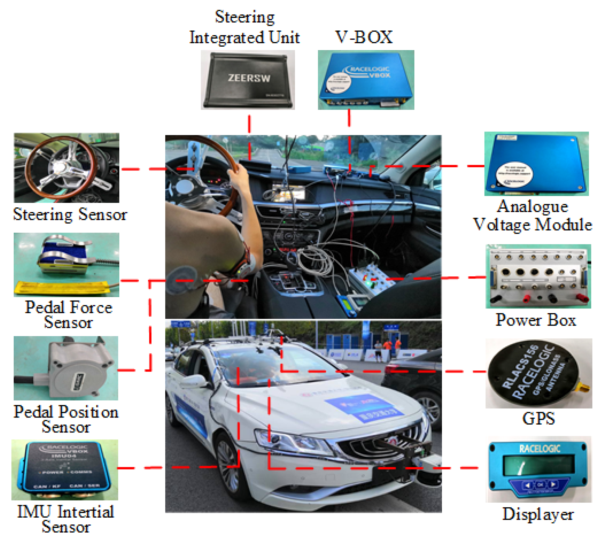
The field experiments are conducted with Chongqing Jiaotong University’s “XinYuan” autonomous vehicle, as shown in Figure 4. All of the vehicle’s signals are collected by a V-BOX integrated device, a vehicle performance test system provided by the British Racelogic company. As shown in Figure 4, the steering wheel angle and torque is measured by a steering sensor mounted on the steering wheel. The pedal force and string position sensors are responsible for collecting the pedal force and stroke. The vehicle’s position and speed information are recorded by the Global Positioning System / Real-time kinematic (GPS/RTK). The vehicle’s state, such as V y , ω γ , e y , ψ , can be collected by the IMU inertial sensor.
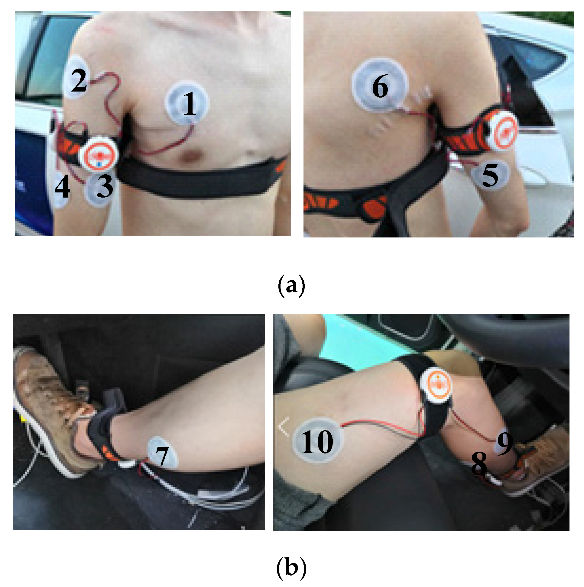
In order to identify the parameters of the arm’s NMS characteristic, a 16-channel EMG measurement instrument supplied by the OT Bio company in Italy is utilized in the experiment. Its sampling rate, resolution rate and bandwidth are 1024 Hz, 16bit and 10 Hz–500 Hz, respectively. The Figure 5 illustrates that primary working muscle groups are monitored by EMG electrodes which are placed and oriented according to surface Electromyography for the non-invasive assessment of muscles (SENIAM) standards [30]. The working muscle groups affecting the driver’s steering ability are listed in Table 3 [31,32].

4.2. Experimental Participants

With the agreement of our university’s academic committee and safety regulatory authorities, three subjects were recruited to take part in the experiments. All of them were male students in college, 26 years old with two years of driving experience. They were volunteers, taking part in the research with no financial reward. All the subjects had experiments performed three times, and the best one is chosen as the experimental data.

4.3. Experimental Scenario

The driving test field of Chongqing Jiaotong University is adopted as our experimental scenario, as shown in Figure 6. The red line represents the trajectory collected by GPS/RTK in the right lane. The complete road section consists of a 326 m double lane with four turning segments, four straight line segments and a ramp segment. The average driving speed on the experimental scenario is restricted to 30 km/h for safety.

4.4. Experimental Procedure

To enhance the confidence of the experimental results, each subject had 20 min of adaptive driving training. Furthermore, sampling frequency of EMG instruments and VBOX were adjusted to be as consistent as possible, both of which were 1024 Hz. Before the experiment, the maximum voluntary contraction (MVC) of each muscle working on steering wheel and pedal was calibrated in order to solve the muscle activation. During the experimental process, three subjects kept holding the steering wheel sensor at the “3–9 o’clock” position, and pressed the brake pedal sensor as shown in Figure 7. Each subject followed the trajectory three times, and the best instance was selected as the experimental data. Noteworthily, an emergency acceleration and braking scenario were designed in order to observe the fast response of the vehicle and muscle signals in S3 segments.

5. Model Verification with Experimental Results

5.1. Activation-to-Force Processing

Muscle force plays a vital role in the research of the driver’s NMS dynamic model. It cannot be measured directly, but can be obtained based on EMG signals. Therefore, a numbers activation-to-force model was proposed [26]. In this paper, the EMG signals are obtained by EMG analysis software “BioLab”. In order to facilitate the analysis of the result, the measurement noise is filtered through 20–400 Hz frequency, followed by average rectified value (RMS) processing. Finally, the linearized time-domain signal is obtained. Noteworthily, the following assumptions are presented: the driver’s muscle characteristic is linear; ignoring the influences of driving fatigue; the length of the tendon contraction is constant; the contribution of each work muscle can be quantified by different weights.
The muscle activation a ( t ) is processed by a nonlinear function:
a ( t ) u ( t ) = R M S ( t ) R M S max
where R M S ( t ) represents the RMS value of EMG at time t after normalization; R M S max infers to the RMS value of EMG in isometric maximum voluntary contraction(MVC); u ( t ) infers to the strength of muscle; a ( t ) indicates the degree of muscle activation.
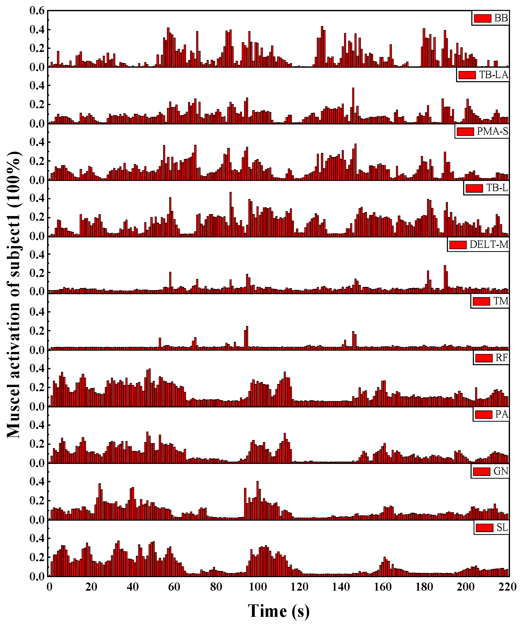
Ten muscle activations are calculated as shown in Figure 8. Evidently, the muscles of Biceps brachii (BB), lateral head of triceps brachii (TB-LA), pectoralis major (PMA-S) and long head of triceps brachii (TB-L) have higher activation which means more contributions for steering movement. Similarly, the rectus femoris (RF) muscle plays the most significant role during speed control.

5.2. Model Verification Results

Using the aforementioned identification algorithm with the experimental results, the key parameters of three subjects are identified in Table 4. The original range of each parameter is derived from reference [33]. All NMS parameters are within a reasonable range, which indicates the model identification results are practicable. In particular, higher stiffness and damping coefficients indicate greater muscle force applied by the driver.
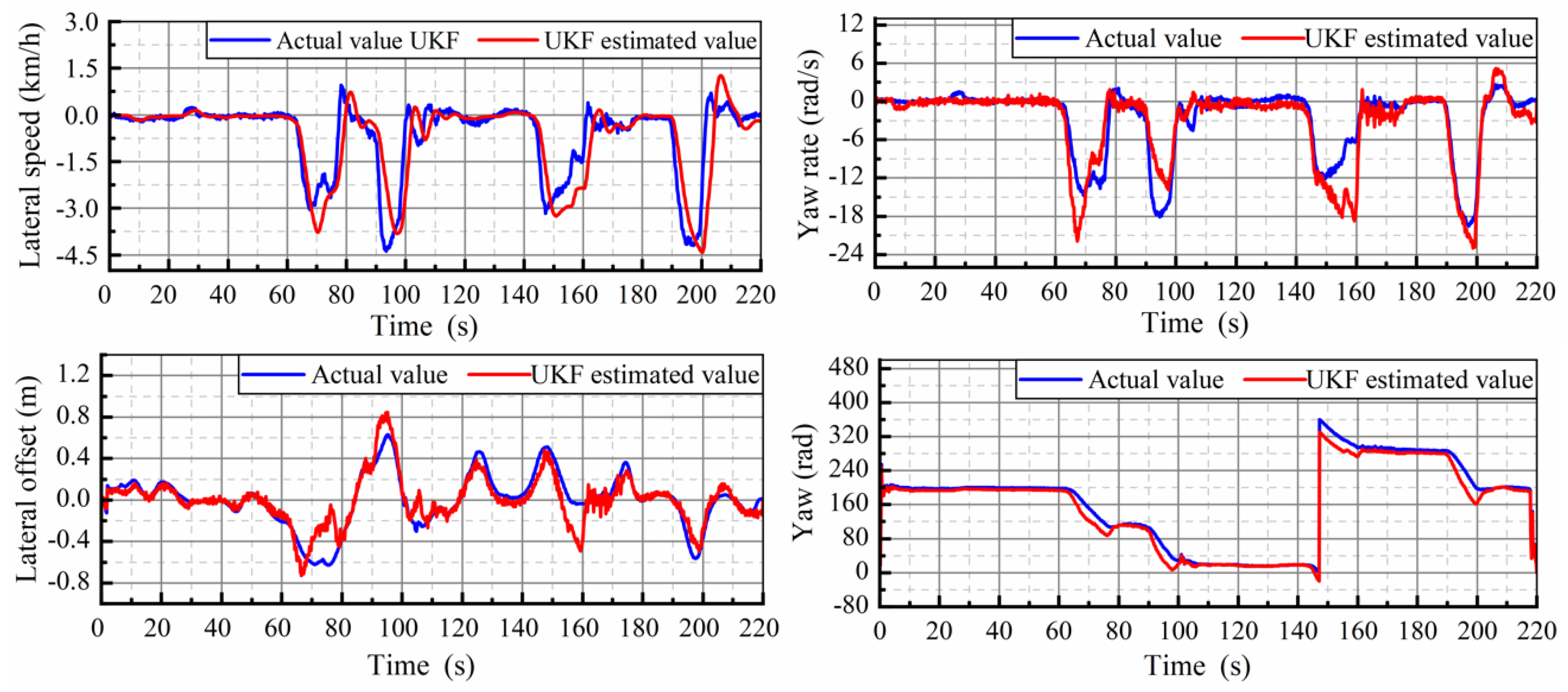
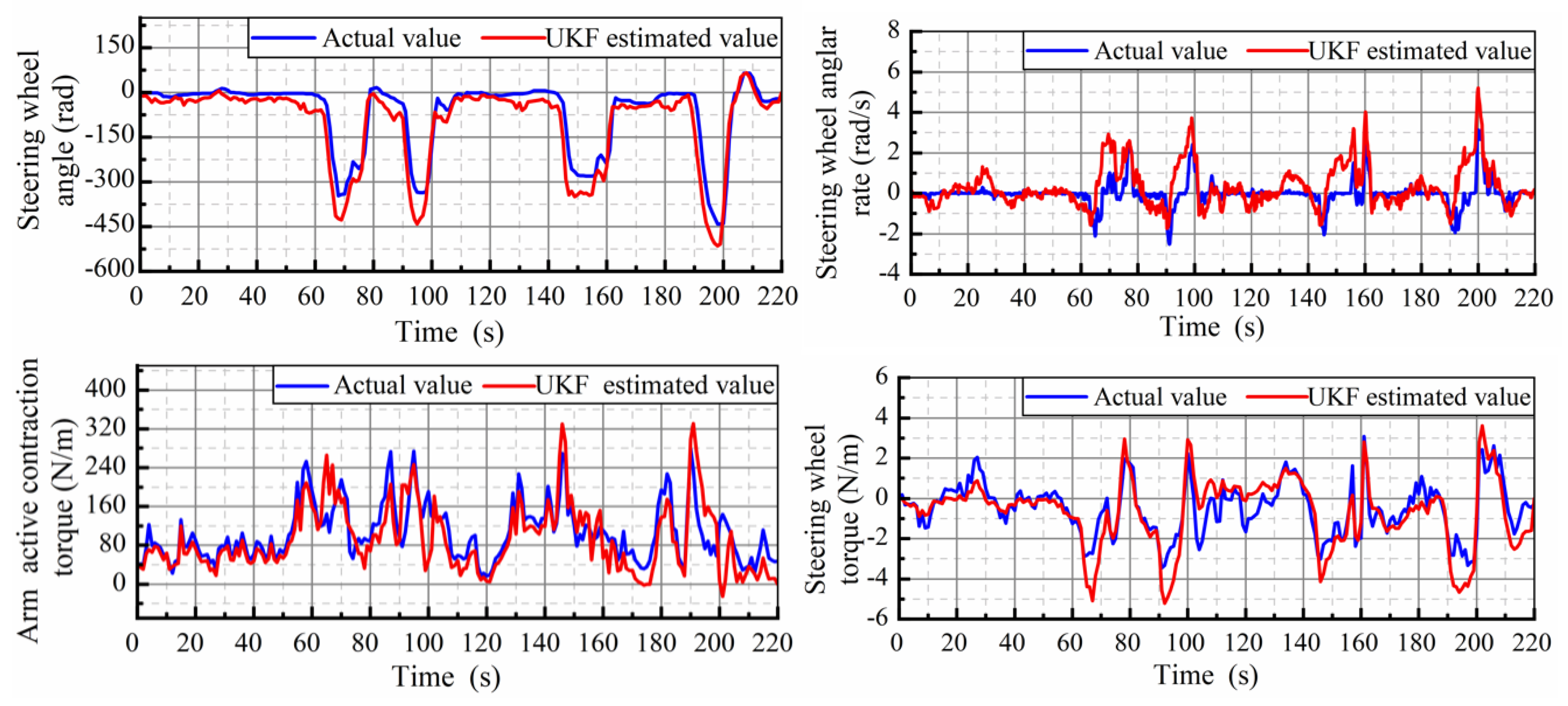
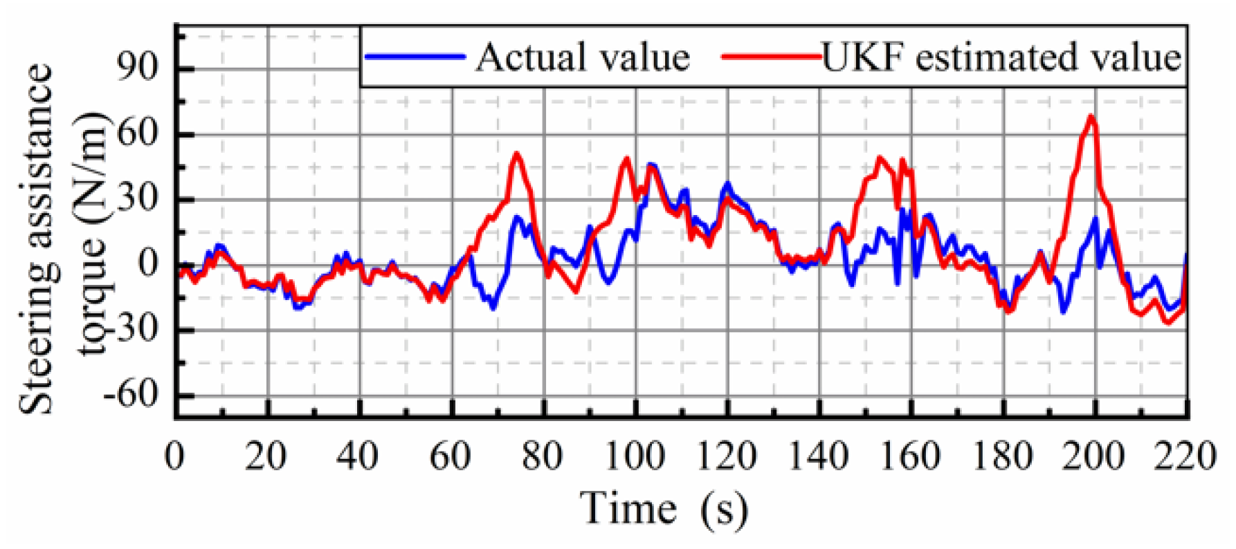
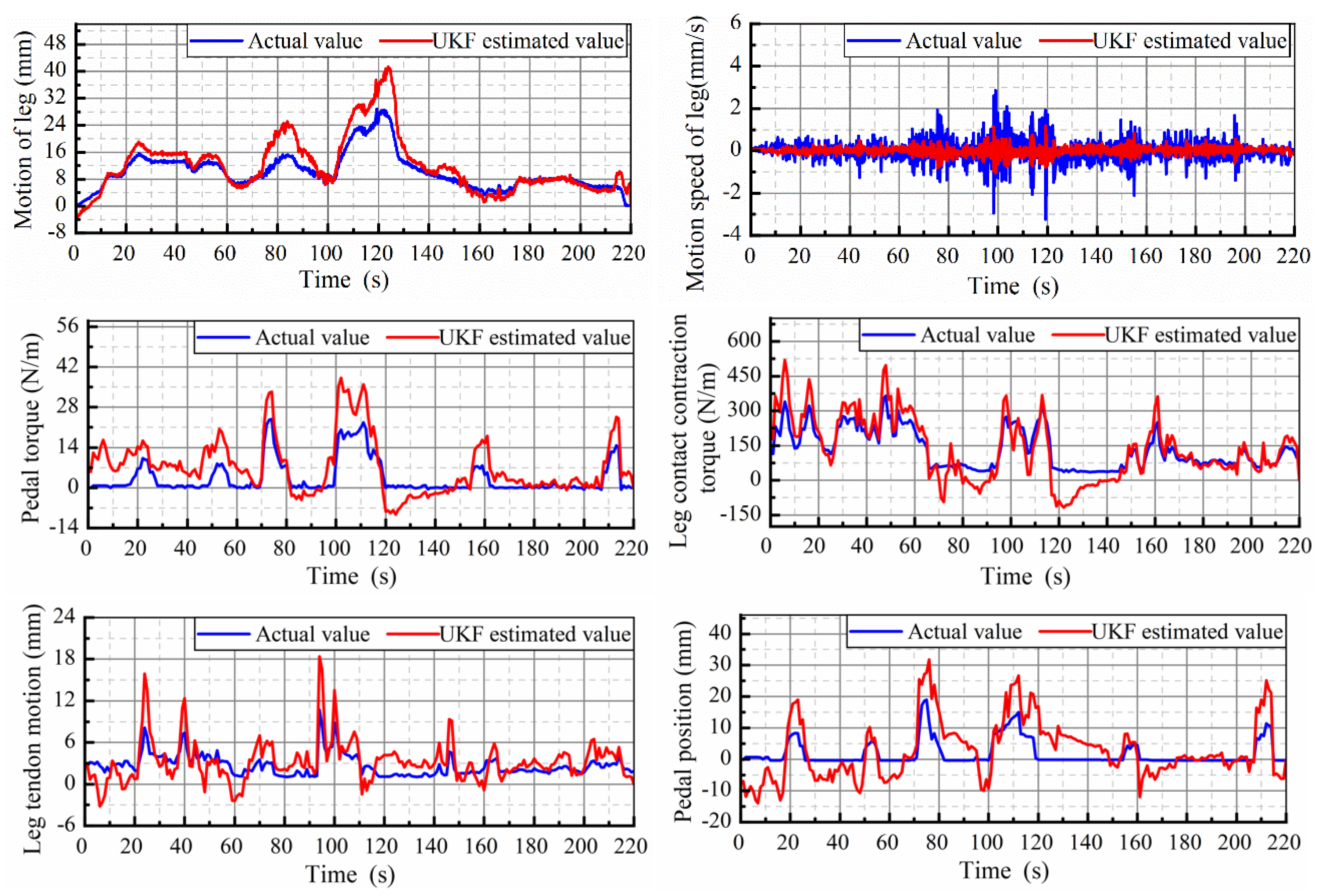
In order to prove the accuracy of the dynamic model and to observe the driver’s personalized behavior, the estimated value with the UKF observer of the first subject and actual value based on the experiment are illustrated in Figure 9, Figure 10 and Figure 11. As can be observed, the UKF estimated value has good consistency with the actual value.

5.3. Model Verification Analysis

In order to verify that the model can observe the driver’s NMS characteristics, the principle of covariance is utilized to analyze the correlation between the actual and observed value of Subject 1. From the statistical principle, the larger var ( t ) value represents the higher degree of data fusion between two groups.
var ( t ) = Σ t = 1 n ( y I ( t ) y ¯ I ) ( y s ( t ) y ¯ s ) n 1
where, y I ( t ) and y s ( t ) represents the initial value and the estimated value which characterizing the subject at time t respectively; y ¯ I and y ¯ s refers to the mean value of the initial value and estimated value respectively.
As shown in Table 5, fifteen correlation coefficients between the actual value and the UKF estimated value are calculated with covariance analysis. From the analysis, all the coefficients greater than 0.7, which indicated that the parameter identification, as well as the UKF observer we proposed, have significant precision.
Furthermore, in order to prove the model’s practicability in reflecting the personalized driver characteristics, the actual value of Subject 1 is compared with three subjects’ estimated values. The covariance analysis results in Figure 12 is normalized for visualization. It can be observed that the histogram of Subject 1 has the highest covariance with the initial state vector. Finally, we can deduce that the HVSC dynamic model we proposed can represent the evolution of personal characteristics.

6. Conclusions

In this paper, a HVSC dynamic model composed by driver’s NMS model, 2DOF vehicle dynamic model and MPC controller is proposed for the shared control of AV. Specifically, the influence of the significant factors of the arms and legs, such as stiffness, damping and inertia are considered into the driver’s NMS model. Field experiments were conducted for the validation of the model. Based on the subsequent experimental results, the HLS algorithm and UKF observer are implemented to identify and estimate the important NMS parameters, respectively. Finally, the covariance analysis shows consistency with the identified parameter of the driver’s NMS characteristics. The results show that the model we proposed has a high level of accuracy with actual value. This paper will serve as a theoretical basis for the control strategy allocation between human and vehicle for L3 class AVs.

Author Contributions

Conceptualization, H.W. and Y.W.; Data curation, X.C. and J.X.; Funding acquisition, H.W.; Supervision, X.C.; Writing—review & editing, Y.W. All authors have read and agreed to the published version of the manuscript.

Funding

This research was funded by [National Key Research and Development Program of China (Grant No. 2018YFB1600500)]; [National Natural Science Foundation of China (Grant No. 51305472)]; [Natural Science Foundation Project of the Chongqing Municipal Science and Technology Commission (Grant No. KJQN201800714)].

Conflicts of Interest

This study has no conflict of interest.

Abbreviations

The following abbreviations are used in this manuscript:
HVSCHuman-vehicle shared control
AVAutonomous vehicle
NMSNeuromuscular
MPCModel predictive control
2DOFTwo-degree-of-freedom
HLSHierarchical least square
UKFUnscented Kalman Filter
GTOGolgi tendon organs
MIMOMulti-input multi-output
EMGElectromyography
MVCMaximum voluntary contraction
RMSAverage rectified value

References

  1. SAE International. Taxonomy and Definitions for Terms related to Driving Autonomous Systems for on-road Motor Vehicles; J3016; SAE International: New York, NY, USA, 2016. [Google Scholar]
  2. Noh, S.; Park, B.; An, K.; Koo, Y.; Han, W. Co-Pilot Agent for Vehicle/Driver Cooperative and Autonomous Driving. ETRI J. 2015, 37, 1032–1043. [Google Scholar] [CrossRef]
  3. Abbink, D.A.; Mulder, M.; Van der Helm, F.C.; Mulder, M.; Boer, E.R. Measuring neuromuscular control dynamics during car following with continuous haptic feedback. IEEE Trans. Syst. Man Cybern. Part B (Cybern.) 2011, 41, 1239–1249. [Google Scholar] [CrossRef] [PubMed]
  4. Olivari, M.; Nieuwenhuizen, F.M.; Bülthoff, H.H.; Pollini, L. Identifying time-varying neuromuscular system with a recursive least-squares algorithm: a Monte-Carlo simulation study. In Proceedings of the 2014 IEEE International Conference on Systems, Man, and Cybernetics (SMC), San Diego, CA, USA, 5–8 October 2014. [Google Scholar]
  5. Golkar, M.A.; Jalaleddini, K.; Tehrani, E.S.; Kearney, R.E. Identification of time-varying dynamics of reflex EMG in the ankle plantar flexors during time-varying, isometric contractions. In Proceedings of the 2015 37th Annual International Conference of the IEEE Engineering in Medicine and Biology Society (EMBC), Milan, Italy, 25–29 August 2015; pp. 6744–6747. [Google Scholar]
  6. Marouf, A.; Pudlo, P.; Sentouh, C.; Djemaï, M. Investigation of the driver’s arm viscoelastic properties during steering vehicle maneuver. IEEE Trans. Syst. Man Cybern. Syst. 2016, 47, 1030–1036. [Google Scholar] [CrossRef]
  7. Lv, C.; Wang, H.; Cao, D.; Zhao, Y.; Auger, D.J.; Sullman, M.; Matthias, R.; Skrypchuk, L.; Mouzakitis, A. Characterization of Driver Neuromuscular Dynamics for Human–Automation Collaboration Design of Automated Vehicles. IEEE/ASME Trans. Mechatron. 2018, 23, 2558–2567. [Google Scholar] [CrossRef] [Green Version]
  8. Bi, L.; Wang, M.; Wang, C.; Liu, Y. Development of a driver lateral control model by integrating neuromuscular dynamics into the queuing network-based driver model. IEEE Trans. Intell. Transp. Syst. 2015, 16, 2479–2486. [Google Scholar] [CrossRef]
  9. Christopher, N.; Cole, D.J. Development of a novel model of human-vehicle steering control incorporating sensory dynamics. Dyn. Veh. Roads Tracks 2016, 43, 57–66. [Google Scholar]
  10. Kolekar, S.; Mugge, W.; Abbink, D. Modeling intradriver steering variability based on sensorimotor control theories. IEEE Trans. Hum. Mach. Syst. 2018, 48, 291–303. [Google Scholar] [CrossRef]
  11. Zhao, Y.; Zhao, F.; Tian, Y. The shared steering controller inspired by the neuromuscular system of drivers. In Proceedings of the 2018 Chinese Control and Decision Conference (CCDC), Shenyang, China, 9–11 June 2018; pp. 3433–3438. [Google Scholar]
  12. Mars, F.; Chevrel, P. Modelling human control of steering for the design of advanced driver assistance systems. Annu. Rev. Control 2017, 44, 292–302. [Google Scholar] [CrossRef]
  13. Lixin, Y.; Huang, Z.; Chaozhong, W. Selection of driving mode for autonomous vehicle based on danger situation recognition. J. South China Univ. Technol. (Nat. Sci. Ed.) 2016, 44, 140–145. [Google Scholar]
  14. Sendler, J.; Trutschel, R.; Augsburg, K.; Schumann, N.P.; Scholle, H.C. Methods of evaluating and developing pedal and brake characteristics. ATZ Worldw. 2009, 111, 60–66. [Google Scholar] [CrossRef]
  15. Endo, K.; Herr, H. A model of muscle–tendon function in human walking at self-selected speed. IEEE Trans. Neural Syst. Rehabil. Eng. 2013, 22, 352–362. [Google Scholar] [CrossRef] [PubMed]
  16. Endo, K.; Paluska, D.; Herr, H. A quasi-passive model of human leg function in level-ground walking. In Proceedings of the 2006 IEEE/RSJ International Conference on Intelligent Robots and Systems, Beijing, China, 9–15 October 2006; pp. 4935–4939. [Google Scholar]
  17. Qashqai, A.; Ehsani, H.; Rostami, M. A hill-based EMG-driven model to estimate elbow torque during flexion and extention. In Proceedings of the 2015 22nd Iranian Conference on Biomedical Engineering (ICBME), Tehran, Iran, 25–27 November 2015; pp. 166–171. [Google Scholar]
  18. Pick, A.; Cole, D. A Mathematical Model of Driver Steering Control Including Neuromuscular Dynamics. J. Dyn. Syst. Meas. Control 2008, 130, 031004. [Google Scholar] [CrossRef]
  19. Pick, A.J.; Cole, D.J. Dynamic properties of a driver’s arms holding a steering wheel. Proc. Inst. Mech. Eng. Part D J. Automob. Eng. 2007, 221, 1475–1486. [Google Scholar] [CrossRef]
  20. Kandel, E.R.; Schwartz, J.H. Principles of Neural Science; McGraw Hill: New York, NY, USA, 2000; Volume 4, pp. 1227–1246. [Google Scholar]
  21. Abbink, D.A. Neuromuscular Analysis of Haptic Gas Pedal Feedback during Car Following. Delft. Ergon. 2008, 51, 1710–1720. [Google Scholar]
  22. Van der Helm, F.C.; Schouten, A.C.; de Vlugt, E.; Brouwn, G.G. Identification of intrinsic and reflexive components of human arm dynamics during postural control. J. Neurosci. Methods 2002, 119, 1–14. [Google Scholar] [CrossRef]
  23. Rajamani, R. Vehicle Dynamics and Control. J. Jpn. Fluid Power Syst. Soc. 2012, 39, 111. [Google Scholar]
  24. Snider, J.M. Automatic Steering Methods for Autonomous Automobile Path Tracking; Tech. Rep. CMU-RITR-09-08; Robotics Institute: Pittsburgh, PA, USA, 2009. [Google Scholar]
  25. Walter, E. Identifiability of State Space Models: With Applications to Transformation Systems; Springer Science & Business Media: Berlin, Germany, 2013. [Google Scholar]
  26. Bai, F.; Chew, C.M.; Li, J.; Shen, B.; Lubecki, T.M. Muscle force estimation method with surface EMG for a lower extremities rehabilitation device. In Proceedings of the 2013 IEEE 13th International Conference on Rehabilitation Robotics (ICORR), Seattle, WA, USA, 24–26 June 2013; pp. 1–6. [Google Scholar]
  27. Ding, F.; Liu, Y.; Bao, B. Gradient-based and least-squares-based iterative estimation algorithms for multi-input multi-output systems. Proc. Inst. Mech. Eng. Part I J. Syst. Control Eng. 2012, 226, 43–55. [Google Scholar] [CrossRef]
  28. Xiang, L.; Xie, L.; Liao, Y.; Ding, R. Hierarchical least squares algorithms for single-input multiple-output systems based on the auxiliary model. Math. Comput. Model. 2010, 52, 918–924. [Google Scholar] [CrossRef]
  29. Ren, H.; Chen, S.; Zhao, Y.; Liu, G.; Yang, L. State observer-based sliding mode control for semi-active hydro-pneumatic suspension. Veh. Syst. Dyn. 2016, 54, 168–190. [Google Scholar] [CrossRef]
  30. Lin, W.; Rong, F.; Cheng, Z.; Xiaowei, Y. Driving fatigue research based on wireless body area network and approximate physiological entropy of physiological signals. Chin. J. Biomed. Eng. 2017, 76, 34–40. [Google Scholar]
  31. Liu, Y.; Ji, X.; Ryouhei, H.; Takahiro, M.; Lou, L. Function of shoulder muscles of driver in vehicle steering maneuver. Sci. China Technol. Sci. 2012, 55, 3445–3454. [Google Scholar] [CrossRef]
  32. Brook, S.; Freeman, R.; Rosala, G.; Campean, F.; Dixon, N. Ergonomic Data measuring system for driver-pedals interaction. SAE Int. J. Passeng. Cars Mech. Syst. 2009, 2, 1071–1078. [Google Scholar] [CrossRef] [Green Version]
  33. Lasschuit, J.; Lam, M.; Mulder, M.; van Paassen, R.; Abbink, D. Measuring and modeling neuromuscular system dynamics for haptic interface design. In Proceedings of the AIAA Modeling and Simulation Technologies Conference and Exhibit, Honolulu, HI, USA, 18–21 August 2008; p. 6543. [Google Scholar]
Figure 1. Human–vehicle shared control (HVSC) dynamics model.
Applsci 10 02626 g001
Figure 2. Vehicle dynamic model.
Applsci 10 02626 g002
Figure 3. Block diagram of HVSC model.
Applsci 10 02626 g003
Figure 4. Field experimental facilities.
Applsci 10 02626 g004
Figure 5. Measured Muscles and the electrode placements. (a) arm muscles, (b) leg muscles.
Applsci 10 02626 g005
Figure 6. Driving experimental scenarios.
Applsci 10 02626 g006
Figure 7. Driving experimental scenario.
Applsci 10 02626 g007
Figure 8. Muscle activation analysis.
Applsci 10 02626 g008
Figure 9. Vehicle state estimated value.
Applsci 10 02626 g009
Figure 10. Arm state estimated value.
Applsci 10 02626 g010aApplsci 10 02626 g010b
Figure 11. Leg state estimated value.
Applsci 10 02626 g011
Figure 12. Covariance analysis of each subject’s state value.
Applsci 10 02626 g012
Table 1. Parameters of driver neuromuscular (NMS) model.
SymbolDescriptionValue
JstSteering wheel inertia0.1395 (kg m2)
BstSteering wheel damper1.56 (Nm s/rad)
KstSteering wheel spring2.29 (Nm/rad)
KaActive stiffness−1920 (Nm/rad)
JdrArm inertia0.172 (kg m2)
BdrArm damping1.032 (Nm s/rad)
KdrArm spring60.707 (Nm/rad)
KrArm reflection stiffness3.423 (Nm s/rad)
BrArm reflection damping1.69 (Nm/rad)
τdelInherent time delay0.04 (s)
KposStretch feedback gain0.52 (Nm/rad)
KtendTendon stiffness2799 (Nm/rad)
f0Eigen-frequency1.1 (Hz)
IsegMotion of the inertia105.5 (g/m2)
KfGTO feedback gain1.18 (Nm/rad)
KvelStretch velocity feedback gain40.4 (Nm/rad)
KintCo-contraction stiffness334 (Nm/rad)
BintCo-contraction damping19.4 (Nm/rad)
KconContact elasticity1033 (Nm/rad)
BconContact viscosity11.2 (Nm /rad)
Table 2. Parameters of the vehicle dynamic model.
SymbolDescriptionValue
IzYaw inertia4192 (kg m2)
vxLongitudinal speed2.29 (m/s)
k1Cornering stiffness of the front tires93360 (N/rad)
k2Cornering stiffness of the rear tires57340 (N/rad)
aFront axle length1.18 (m)
bRear axle length1.58 (m)
mBody mass1498 (kg)
xlLook-ahead distance12 (m)
nrswSteering gear ratio18
Table 3. Measured muscle groups.
NumberMuscle NameFunctionality
1Sternocostal portion of Pectoralis major (PMA-S)Steering right
2Middle deltoid (DELT-M)Steering right
3Biceps brachii (BB)Steering left
4Lateral head of triceps brachii (TB-LA)Steering right
5Long head of triceps brachii (TB-L)Steering left
6Teres major (TM)Steering left
7Rectus femoris (RF)Speed control
8Patellar anterior (PA)Speed control
9Gastrocnemius muscle (GN)Speed control
10Soleus muscle (SL)Speed control
Table 4. Identified parameter of NMS characteristics.
SubjectRangeInitialSub1Sub2Sub3
Prameter
Jdr (kg/m2)[0.03~0.14]0.1720.1620.0970.125
Bdr (Nm/rad)[0.1~2.5]1.0320.9890.910.932
Kdr (Nm/rad)[20~90]60.70758.87349.10552.34
Br (Nm s/rad)[0.5~2]1.691.5320.91.472
Kr (Nm/rad)[2~30]3.4242.5022.152.27
Ktend (Nm/rad)[1799–3988]2799277120962459
Kf (Nm/rad)[−0.81~1.78]1.181.271.361.32
Kvel (Nm/rad)[−0.40~48.6]40.441.5133.1238.74
Kint (Nm/rad)[191~505]334318381397
Bint (Nm/rad)[16~22.2]19.419.316.117.8
Kcon (Nm/rad)[615~1143]10331022893921
Bcon (Nm/rad)[10.6~11.7]11.211.3210.8710.91
Table 5. Covariance analysis results between the actual value and Unscented Kalman Filter (UKF) estimated value.
No.ParameterCoefficientNo.ParameterCoefficient
1Lateral speed0.86219Steering assistance torque0.7156
2Yaw rate0.824610Motion of leg0.82323
3Lateral offset0.765311Movement speed of leg0.74421
4Yaw0.895612Pedal torque0.7021
5Steering wheel angle0.866313Leg contraction torque0.74421
6Steering wheel angular rate0.842114Leg tendon motion0.746
7Arm active contraction torque0.7342115Pedal position0.716
8Steering wheel torque0.8646