Implementation of Fault-Tolerant Control for a Robot Manipulator Based on Synchronous Sliding Mode Control

Abstract

In this paper, an active fault-tolerant control for a robot manipulator based on synchronous sliding mode is proposed. As the synchronization errors approach zero, the joint errors tend to become equal and also approach zero. Therefore, the synchronization technique is inherently effective for a fault-tolerant controller. To demonstrate such a system, the following implementation is presented. First, an estimator was designed with an extended state observer to estimate uncertainties/disturbances along with faults/failures. The estimator signal was used for an online compensator in the controller. A fault-tolerant controller with a combination of synchronous sliding mode technique and estimator was proposed. The stability of the system was established using Lyapunov theory. Finally, fault tolerant control was implemented in a three degree-of-freedom robot manipulator and compared to the conventional sliding mode control. This comparison shows the effectiveness of the proposed active fault-tolerant control with synchronous sliding mode technique.

1. Introduction

During the past two decades, fault detection and fault-tolerant control (FTC) have become attractive research subjects that can be used to improve system reliability and guarantee system stability in all situations. Implementation of fault-tolerant control in robot manipulators has encountered a number of challenges due to high nonlinearities, dynamic uncertainties, and external disturbances. In addition, the time delay inherent to mechanical systems also affects the performance of FTC. FTC strategies can be divided into two categories: passive FTC (PFTC) [1,2] and active FTC (AFTC) [3,4]. In PFTC, the control performances mainly depend on the robust capability dealing with uncertainties/disturbances of the controller such as sliding mode control [5] or adaptive control [6,7]. In this strategy, the controller does not have a faults estimation process. The advantage of PFTC is the fast response when faults occur, because it does not need time to estimate faults. However, the ability to deal with high magnitude faults is limited. Unlike PFTC, AFTC reconfigures the control system based on the estimation process. The fault information from the estimation process is used to compensate the conventional controller. The disadvantage of this strategy is slow response after faults occur, which leads to the occurrence of a picking phenomenon, because the controller needs the time to estimate the faults. Most studies in active fault-tolerant control [3,8,9] have focused on increasing the ability to deal with uncertainties/disturbances of the controller. Therefore, the performance degradation of the system with the AFTC strategy due to the slow response still remains an open problem. However, AFTC has better ability when dealing with high magnitude faults than PFTC. As above-mentioned, using PFTC or AFTC depends on the characteristics of the system and type of faults. In robot manipulator control, AFTC generally outperforms PFTC because AFTC includes a fault estimation (FE) step. The estimated faults can be compensated for by online controller reconfiguration. In this way, the stability and acceptable performance of the robot can be maintained.

In AFTC, the quality of the fault-tolerant control depends on the accuracy of both FE and the system reconfiguration after faults occur. In fault estimation processing, several techniques [10,11,12,13,14,15] have been used. The parameter estimation method [10] is used to early detect faults applied for dynamic linear and nonlinear systems. The parity relations [11] used the parity equations to be combined with the least-square method to estimate faults. The sliding mode observers [12] have been given lot of attention by researchers. However, this method is limited in real applications due to the disadvantages such as the chattering phenomenon, the requirement of the knowledge of the fault’s bound to choose the observer parameters, and the stability issue. In addition, other techniques such as the Kalman Filter [13], zonotope [14], and nonlinear observer [15] were developed to estimate the faults as well as uncertainties/disturbances. After faults are estimated, they are compensated for by using various control strategies [16,17,18]. In this study, an extended state observer [19] was adopted for on-line observation of the dynamic uncertainties, disturbances, and faults. An extended state observer (ESO) is a simple technique for estimating faults in which simply adjusting the observer parameters leads to simple application in real systems, and the observer can detect and isolate faults without a fault diagnosis process. In addition, the upper bound of faults does not have to be exactly known in the design of ESO.

A synchronization technique based on cross-error was first introduced by Y. Koren [20] in the 1980s for a computerized numerical control (CNC) machine. In his idea, a CNC with independent axes control is extended to enable the control of each access to consider the effects of the other axes through cross-errors. L. Feng et al. [21] proposed cross-coupling control for mobile robots. He suggested that minimization of the most significant error leads to coordination of the motion of the two wheels. Lu Ren et al. [22] introduced synchronization errors, a new type of cross-coupling error, in controlling a parallel robot manipulator. Synchronization control has also been applied in multi-robot cooperation [23,24]. Synchronization techniques combined with the sliding mode method have attracted the interest of many researchers. The position and velocity synchronization error have been used instead of position and velocity error, respectively, in sliding mode control structures [25]. Zhang et al. [26] also proposed a robust synchronous control based on a sliding mode variable structure for multi-motors. These studies [23,24,25,26] have applied synchronization control techniques to a parallel robot, multi-robot cooperation, and multi-motors to improve trajectory tracking performance. This work is interested in addressing a slow response issue by using the synchronization control technique, which can make the position error at each joint equal. Therefore, the system can quickly respond to a fault due to the constraint of synchronization control before the controller has the feedback information from the fault estimation process. Considering the dynamic coupling effects between actuators and the upper bound of the uncertainties, the effectiveness of synchronization techniques might be somewhat limited to improvements of the trajectory tracking control. However, synchronization techniques become more effective in critical conditions, which lead to applying synchronization techniques to the fault-tolerant control. The contributions of this paper are summarized as follows:

(1)

Synchronization techniques are applied to fault-tolerant control for robot manipulators for the first time. Compared to active fault-tolerant control using conventional sliding mode control, the proposed system has achieved higher accuracy, robustness, and faster system reconfiguration when faults occur. These results confirm that synchronization techniques are very effective in fault-tolerant control.

(2)

The stability of the proposed AFTC with the synchronous sliding mode technique is demonstrated using analysis via Lyapunov theory.

(3)

Based on the extended state observer, the proposed controller can easily monitor faults without detection and isolation processes. This feature is helpful in maintenance systems as well as maintenance planning systems.

(4)

The experimental results show that the proposed control can be easily applied to a real system with robust performance.

In this paper, we present a fault-tolerant control for robot manipulators based on synchronous sliding mode control. Section 2 describes the robot dynamic models. Section 3 explains the process of fault estimation with the extended state observer for robot manipulators. In Section 4, a fault-tolerant control based on synchronous sliding mode control is presented and its stability is demonstrated. In Section 5, a simulation study of the proposed fault-tolerant control for a 3-DOF manipulator was conducted to show the method’s effectiveness. In Section 6, real implementation of the FTC for a 3-DOF FARA AT2 robot was carried out in two cases: a single fault and multiple faults. Finally, conclusions are discussed in Section 7.

2. Dynamics Model of Robot Manipulators

The dynamics of an n-degree of freedom robot manipulator was defined [27] as

$$M(q)\ddot{q}+C(q,\dot{q})\dot{q}+G(q)+F_f(\dot{q})=\tau$$

(1)

where $\ddot{q},\dot{q},q\in {\Re }^n$ are the vectors of joint acceleration, velocity, and position, respectively. $M(q)\in {\Re }^{n\times n}$, $C(q,\dot{q})\in {\Re }^n$, and $G(q)\in {\Re }^n$ represent the inertia matrix, the centripetal and Coriolis matrix, and the gravitation force, respectively. $F_f\in {\Re }^n$ is the friction term and $\tau \in {\Re }^n$ is the torque at the joints.

In practice, the dynamics model of a robot is not exactly known, so Equation (1) can be written as

$$(\mathbf{M}(q)+\Delta M(q))\ddot{q}+(\mathbf{C}(q,\dot{q})+\Delta C(q,\dot{q}))\dot{q}+(\mathbf{G}(q)+\Delta G(q))+({\mathbf{F}}_f(\dot{q})+\Delta F_f(\dot{q}))+\delta =\tau$$

(2)

where $\Delta M,\Delta C,\Delta G$ and $\Delta F$ are unknown dynamic uncertainties and $\delta$ is the unknown external disturbances. $\mathbf{M}(q), \mathbf{C}(q,\dot{q}), \mathbf{G}(q) \mathrm{and} \mathbf{F}(\dot{q})$ are estimated of $M(q),C(q,\dot{q}),G(q) \mathrm{and} F(\dot{q})$. Thus, Equation (2) can be simply rewritten as

$$\mathbf{M}(q)\ddot{q}+\mathbf{C}(q,\dot{q})\dot{q}+\mathbf{G}(q)+{\mathbf{F}}_f(\dot{q})+\mathsf{\psi }(q,\dot{q},\ddot{q},t)=\tau$$

(3)

where $\mathsf{\psi }(q,\dot{q},\ddot{q},t)=\Delta M\ddot{q}+\Delta C\dot{q}+\Delta G+\Delta F+\delta$.

Properties: 

$$\begin{array}{l}{\mu }_1{I}_n\le \mathbf{M}(q)\le {\mu }_2{I}_n\\ \frac{1}{{\mu }_1}{I}_n\le {\mathbf{M}}^{-1}(q)\le \frac{1}{{\mu }_2}{I}_n\end{array}$$

In general, actuator faults can be divided into two types: bias faults and gain faults. In a robot manipulator, these are known as loss of effectiveness and lock-in-place faults. In practice, both kinds of actuator faults commonly occur. Actuator bias faults can be generally described as

$${\tau }^b=\tau +\mathbf{f}(t)$$

(4)

where $\mathbf{f}(t)={[f_1,f_2,\dots f_n]}^T\in {\Re }^n(i=1,2,\dots ,n)$ denotes a bounded signal. ${\tau }^b$ is the torque at the joint when faults occur. Due to loss of effectiveness, actuator gain fault can be described as

$${\tau }^g=(I-\mathsf{\rho }(t))\tau$$

(5)

where $\mathsf{\rho }(t)=diag({\rho }_i(t))\in {\Re }^{n\times n}$, $0\le {\rho }_i(t)<1$$(i=1,2,\dots ,n)$, which is unknown, denotes the remaining control rate. $I\in {\Re }^{n\times n}$ is the identity matrix. Therefore, the total torque including two kinds of actuator faults can be comprehensively described as

$${\tau }^t=(I-\mathsf{\rho }(t))\tau +\mathbf{f}(t)(t>t_f)$$

(6)

where $t_f$ is the time of occurrence of each fault.

Substituting Equation (6) into Equation (3), the dynamics model of an n-degree of freedom robot manipulator with actuator faults can be written as

$$\mathbf{M}(q)\ddot{q}+\mathbf{C}(q,\dot{q})\dot{q}+\mathbf{G}(q)+{\mathbf{F}}_f(\dot{q})+\mathsf{\psi }(q,\dot{q},\ddot{q},t)=(I-\mathsf{\rho }(t))\tau +\mathbf{f}(t)$$

(7)

Assumption 1.

There exist known positive constants${\overline{\rho }}_i,{\overline{\overline{\rho }}}_i,\overline{\mathbf{f}},\overline{\overline{\mathbf{f}}}$such that$\left|{\rho }_i(t)\right|\le {\overline{\rho }}_i$,$\left|{\dot{\rho }}_i(t)\right|\le {\overline{\overline{\rho }}}_i$,$\left|\mathbf{f}\right|\le \overline{\mathbf{f}}$, and$\left|\dot{\mathbf{f}}\right|\le \overline{\overline{\mathbf{f}}}$.

3. Fault Estimation Using an Extended State Observer

In this section, an extended state observer of uncertainties/disturbances and faults/failures is presented.

The dynamic model of the robot manipulator of Equation (7) can be rewritten in state space as

$$\ddot{q}={\mathbf{M}}^{-1}(q)(\tau -\mathbf{H}(q,\dot{q}))-{\mathbf{M}}^{-1}(q)\zeta (q,\dot{q},\ddot{q},\tau ,t)$$

(8)

where $\mathbf{H}(q,\dot{q})=\mathbf{C}(q,\dot{q})q+\mathbf{G}(q)+{\mathbf{F}}_f(\dot{q})$. $\zeta (q,\dot{q},\ddot{q},\tau ,t)=\mathsf{\rho }(t)\tau +\mathsf{\psi }(q,\dot{q},\ddot{q},t)-\mathbf{f}(t)$ represents the uncertainties/disturbances and faults/failures.

In state space, the dynamic model of Equation (8) becomes

$$\{\begin{array}{l}{\dot{x}}_1=x_2\\ {\dot{x}}_2=f(x_1,x_2,\tau )+\varphi (x_1,x_2,\tau ,t)\end{array}$$

(9)

where $x_1=q\in {\Re }^n$, $x_2=\dot{q}\in {\Re }^n$, $f(x_1,x_2,\tau )={\mathbf{M}}^{-1}(q)(\tau -\mathbf{H}(q,\dot{q}))$, and $\varphi (x_1,x_2,\tau ,t)=-{\mathbf{M}}^{-1}(q)\zeta (q,\dot{q},\ddot{q},\tau ,t)$.

An extended state observer [19] is given as

$$\{\begin{array}{l}{\dot{\stackrel{⌢}{x}}}_1={\stackrel{⌢}{x}}_2+\frac{{\alpha }_1}{\epsilon }(x_1-{\stackrel{⌢}{x}}_1)\\ {\dot{\stackrel{⌢}{x}}}_2=\stackrel{⌢}{f}(x_1,{\stackrel{⌢}{x}}_2,\tau )+\frac{{\alpha }_2}{{\epsilon }^2}(x_1-{\stackrel{⌢}{x}}_1)+\stackrel{⌢}{\varphi }\\ \dot{\stackrel{⌢}{\varphi }}=\frac{{\alpha }_3}{{\epsilon }^3}(x_1-{\stackrel{⌢}{x}}_1)\end{array}$$

(10)

where ${\stackrel{⌢}{x}}_1,{\stackrel{⌢}{x}}_2,\stackrel{⌢}{f}$ and $\stackrel{⌢}{\varphi }$ are estimates of $x_1,x_2,f$ and $\varphi$, respectively; ${\alpha }_1,{\alpha }_2$, and ${\alpha }_3$ are positive constants; polynomial $s^3+{\alpha }_1{s}^2+{\alpha }_{2}s+{\alpha }_3$ is Hurwitz; and $0<\epsilon <1$.

Theorem 1.

Considering the system (9) with observer (10) and satisfying$0<\epsilon <1$and$\left|\dot{\varphi }\right|\le L$, then${\stackrel{⌢}{x}}_1(t)\to x_1(t)$,${\stackrel{⌢}{x}}_2(t)\to x_2(t)$and$\stackrel{⌢}{\varphi }(q,\dot{q},t)\to \varphi (q,\dot{q},t)$as$t\to \infty$.

Proof. 

We define the observer error as $\tilde{e}={[{\tilde{e}}_1,{\tilde{e}}_2,{\tilde{e}}_3]}^T$ where ${\tilde{e}}_1=(x_1-{\stackrel{⌢}{x}}_1)/{\epsilon }^2$, ${\tilde{e}}_2=(x_2-{\stackrel{⌢}{x}}_2)/\epsilon$ and ${\tilde{e}}_3=\varphi -\stackrel{⌢}{\varphi }$. From assumption 1 and Equation (9), it can be seen that there will exist a value $L$ satisfying $\left|\dot{\varphi }\right|\le L$. The value of $L$ does not need to be exactly known. The function $f$ is a known function of $(x_1,x_2,\tau )$, and we can take $\stackrel{⌢}{f}=f$ as [19].

We define the Lyapunov function as

$$V=\epsilon {\tilde{e}}^{T}P\tilde{e}$$

(11)

where the matrix P is unique, symmetric, and positive.

The time derivative of V in Equation (11) is

$$\dot{V}=\epsilon {\dot{\tilde{e}}}^{T}P\tilde{e}+\epsilon {\tilde{e}}^{T}P\dot{\tilde{e}}$$

(12)

where

$$\begin{array}{ll}\epsilon \dot{\tilde{e}}& =\left[\begin{array}{c}\epsilon {\dot{\tilde{e}}}_1\\ \epsilon {\dot{\tilde{e}}}_2\\ \epsilon {\dot{\tilde{e}}}_3\end{array}\right]=\left[\begin{array}{c}\frac{{\dot{x}}_1-{\dot{\stackrel{⌢}{x}}}_1}{\epsilon }\\ \epsilon \frac{{\dot{x}}_2-{\dot{\stackrel{⌢}{x}}}_2}{\epsilon }\\ \epsilon (\dot{\varphi }-\dot{\stackrel{⌢}{\varphi }})\end{array}\right]=\left[\begin{array}{c}-\frac{{\alpha }_1}{{\epsilon }^2}(x_1-{\stackrel{⌢}{x}}_1)+\frac{1}{\epsilon }(x_2-{\stackrel{⌢}{x}}_2)\\ -\frac{{\alpha }_2}{{\epsilon }^2}(x_1-{\stackrel{⌢}{x}}_1)+(\varphi -\stackrel{⌢}{\varphi })\\ \epsilon \dot{\varphi }-\frac{{\alpha }_3}{{\epsilon }^2}(x_1-{\stackrel{⌢}{x}}_1)\end{array}\right]\\ & =\left[\begin{array}{c}-{\alpha }_1{\tilde{e}}_1+{\tilde{e}}_2\\ -{\alpha }_2{\tilde{e}}_1+{\tilde{e}}_3\\ -{\alpha }_3{\tilde{e}}_1+\epsilon \dot{\varphi }\end{array}\right]=A\tilde{e}+\epsilon B\dot{\varphi }\end{array}$$

(13)

where

$$A=\left[\begin{array}{ccc}-{\alpha }_1& 1& 0\\ -{\alpha }_2& 0& 1\\ -{\alpha }_3& 0& 0\end{array}\right]\hspace{1em}\mathrm{and}\hspace{1em}B=\left[\begin{array}{c}0\\ 0\\ 1\end{array}\right].$$

It is easy to see that A is Hurwitz, so there is a symmetric positive definite matrix Q satisfying the Lyapunov equation

$$A^{T}P+PA=-Q$$

(14)

Substituting Equations (13) and (14) into Equation (12), we have

$$\begin{array}{ll}\dot{V}& =\epsilon {\dot{\tilde{e}}}^{T}P\tilde{e}+\epsilon {\tilde{e}}^{T}P\dot{\tilde{e}}\\ & ={(A\tilde{e}+\epsilon B\dot{\varphi })}^{T}P\tilde{e}+{\tilde{e}}^{T}P(A\tilde{e}+\epsilon B\dot{\varphi })\\ & ={\tilde{e}}^T{A}^{T}P\tilde{e}+\epsilon {(B\dot{\varphi })}^{T}P\tilde{e}+{\tilde{e}}^{T}PA\tilde{e}+\epsilon {\tilde{e}}^{T}PB\dot{\varphi }\\ & ={\tilde{e}}^T(A^{T}P+PA)\tilde{e}+2\epsilon {\tilde{e}}^{T}PB\dot{\varphi }\\ & \le -{\tilde{e}}^{T}Q\tilde{e}+2\epsilon \Vert PB\Vert \cdot \Vert \tilde{e}\Vert \cdot \left|\dot{\varphi }\right|\end{array}$$

(15)

where L is the positive constant that satisfies $\left|\dot{\varphi }\right|\le L$. Therefore,

$$\dot{V}\le -{\lambda }_{\min }(Q){\Vert \tilde{e}\Vert }^2+2\epsilon L\Vert PB\Vert \Vert \tilde{e}\Vert$$

(16)

To guaranty stability of the system, we impose $\dot{V}\le 0$, so the observer error convergence is given as

$$\Vert \tilde{e}\Vert \le \frac{2\epsilon L\Vert PB\Vert }{{\lambda }_{\min }(Q)}$$

(17)

 □

4. Fault Tolerant Control with Synchronous Sliding Mode Control

In this section, the fault-tolerant control based on synchronous sliding mode control is proposed. Some definitions are necessary to propose the fault-tolerant control law. Synchronization error [28] is given as

$$\begin{array}{c}{\epsilon }_1={\psi }_1{e}_1-{\psi }_2{e}_2\\ {\epsilon }_2={\psi }_2{e}_2-{\psi }_3{e}_3\\ ⋮\\ {\epsilon }_{n-1}={\psi }_{n-1}{e}_{n-1}-{\psi }_n{e}_n\\ {\epsilon }_n={\psi }_n{e}_n-{\psi }_1{e}_1\end{array}$$

(18)

where $e_i(i=1,2,\dots ,n)$ is the error at each joint and ${\psi }_i(i=1,2,\dots ,n)$ is the corresponding positive gain. The synchronization control goal [28] is stated as $e_1=e_2=e_3=\dots =e_n$ and $e_i\to 0$ at $t\to \infty$. In a traditional controller, only the position error converges to zero, but in the synchronization control, the kinematic relationship among the errors as well as the position error converges to zero. For ease of practical implementation, ${\psi }_i=1$ is chosen. Then, Equation (18) can be written as

$$\begin{array}{c}{\epsilon }_1=e_1-e_2\\ {\epsilon }_2=e_2-e_3\\ ⋮\\ {\epsilon }_n={\epsilon }_n-{\epsilon }_1\end{array}$$

(19)

Cross-coupling error [28] is given as

$$\begin{array}{c}{\xi }_1={\gamma }_1{\epsilon }_1-{\gamma }_n{\epsilon }_n\\ {\xi }_2={\gamma }_2{\epsilon }_2-{\gamma }_1{\epsilon }_1\\ ⋮\\ {\xi }_n={\gamma }_n{\epsilon }_n-{\gamma }_{n-1}{\epsilon }_{n-1}\end{array}$$

(20)

where ${\gamma }_i(i=1,2,\dots ,n)$ is the positive gain. In this paper, ${\gamma }_i=1$ was chosen. Then, Equation (20) can be written as

$$\begin{array}{c}{\xi }_1={\epsilon }_1-{\epsilon }_n\\ {\xi }_2={\epsilon }_2-{\epsilon }_1\\ ⋮\\ {\xi }_n={\epsilon }_n-{\epsilon }_{n-1}\end{array}$$

(21)

The coupling position error [28], which includes the position and synchronization errors, is defined as

$$E_i={\mathsf{\mu }}_i{e}_i+{\eta }_i{\displaystyle \int {\xi }_i}dt$$

(22)

where ${\eta }_i$ and ${\mathsf{\mu }}_i$ are positive gains. The synchronous sliding surface [26] is defined as

$$S=\dot{E}+cE$$

(23)

where $S={[S_1,S_2,\dots ,S_n]}^T\in {\Re }^n$;$c\in {\Re }^{n\times n}$ is the diagonal positive matrix; and $E={[E_1,E_2,\dots ,E_n]}^T\in {\Re }^n$ with $E_i$ defined in Equation (22). For ease of implementation, the synchronous sliding surface is rewritten as

$$s=\dot{e}+ce+\alpha \xi +\kappa {\displaystyle \int \xi }dt$$

(24)

where $s={[S_1/{\mathsf{\mu }}_1,S_2/{\mathsf{\mu }}_2,\dots ,S_n/{\mathsf{\mu }}_n]}^T\in {\Re }^n$, $\alpha =diag({\eta }_i/{\mathsf{\mu }}_i)\in {\Re }^{n\times n}$ and $\kappa =diag(c_i{\eta }_i/{\mathsf{\mu }}_i)\in {\Re }^{n\times n} (i=1,2,\dots ,n)$ are positive gain matrices.

Here, the fault-tolerant control law is proposed as

$$\tau ={\tau }_0+{\tau }_{SSMC}+{\tau }_{ob}$$

(25)

where

${\tau }_0=\mathbf{M}(q){\ddot{q}}_d+\mathbf{H}(q,\dot{q})$, ${\tau }_{ssmc}=\mathbf{M}(q)(c\dot{e}+\alpha \dot{\xi })+k_{1}sgn(s)+k_{2}s+k_3\xi$, and ${\tau }_{ob}=-\mathbf{M}(q)\stackrel{⌢}{\varphi }$.

Theorem 2.

The system described in (7), using controller specified in (25) guarantees that$e\to 0 and \epsilon \to 0$as time$t\to \infty$under the condition$k_3>\kappa$.

Proof. 

Following [22], the Lyapunov function can be selected as

$$V=\frac{1}{2}{s}^{T}s+\frac{1}{2}{\displaystyle \sum _{i=1}^n{\mathsf{\Lambda }}_{\epsilon }{\epsilon }_i^2}+\frac{1}{2}{\displaystyle \sum _{i=1}^n{\kappa }_{\epsilon }{\mathsf{\Lambda }}_{\epsilon }{\left({\displaystyle \int {\epsilon }_i-{\epsilon }_{i-1}}\right)}^2}dt\ge 0$$

(26)

The time derivative of V is therefore

$$\begin{array}{ll}\dot{V}& =s^T\dot{s}+{\displaystyle \sum _{i=1}^n{\dot{\epsilon }}_i{\mathsf{\Lambda }}_{\epsilon }\epsilon +{\displaystyle \sum _{i=1}^n{\kappa }_{\epsilon }{\mathsf{\Lambda }}_{\epsilon }({\epsilon }_i-{\epsilon }_{i-1}){\displaystyle \int ({\epsilon }_i-{\epsilon }_{i-1})}}}dt\\ & =A_1+{\displaystyle \sum _{i=1}^n{\dot{\epsilon }}_i{\mathsf{\Lambda }}_{\epsilon }\epsilon +{\displaystyle \sum _{i=1}^n{\kappa }_{\epsilon }{\mathsf{\Lambda }}_{\epsilon }({\epsilon }_i-{\epsilon }_{i-1}){\displaystyle \int ({\epsilon }_i-{\epsilon }_{i-1})}}}dt\end{array}$$

(27)

where $A_1=s^T\dot{s}$. ${\mathsf{\Lambda }}_{\epsilon }$ and ${\kappa }_{\epsilon }$ are positive gain.

Differentiation of Equation (24) gives

$$\dot{s}=\ddot{e}+c\dot{e}+\alpha \dot{\xi }+\kappa \xi ={\ddot{q}}_d-\ddot{q}+c\dot{e}+\alpha \dot{\xi }+\kappa \xi$$

(28)

Substituting Equation (8) into Equation (28) yields

$$\dot{s}={\ddot{q}}_d+c\dot{e}+\alpha \dot{\xi }+\kappa \xi -{\mathbf{M}}^{-1}(q)(\tau -\mathbf{H}(q,\dot{q}))-{\mathbf{M}}^{-1}(q)\zeta (q,\dot{q},\tau ,t)$$

(29)

Substituting Equation (25) into Equation (29), we have

$$\begin{array}{ll}\dot{s}& ={\ddot{q}}_d+c\dot{e}+\alpha \dot{\xi }+\kappa \xi -{\mathbf{M}}^{-1}(q)\{\mathbf{M}(q){\ddot{q}}_d+\mathbf{H}(q,\dot{q})+\mathbf{M}(q)(c\dot{e}+\alpha \dot{\xi })+k_{1}sgn(s)+k_{2}s+k_3\xi \\ & -\mathbf{M}(q)\stackrel{⌢}{\varphi }-H(q,\dot{q})\}+{\mathbf{M}}^{-1}(q)\zeta (q,\dot{q},\ddot{q},\tau ,t)\\ & =-{\mathbf{M}}^{-1}(q)k_{1}sgn(s)-{\mathbf{M}}^{-1}(q)k_{2}s-(\kappa +{\mathbf{M}}^{-1}(q)k_3)\xi +\stackrel{⌢}{\varphi }+{\mathbf{M}}^{-1}(q)\zeta (q,\dot{q},\ddot{q},\tau ,t)\end{array}$$

(30)

It can be seen that when $\stackrel{⌢}{\varphi }\to \varphi$ at $t\to \infty$$\stackrel{⌢}{\varphi }=-{\mathbf{M}}^{-1}(q)\zeta (q,\dot{q},\tau ,t)$ then Equation (30) becomes

$$\dot{s}={\mathbf{M}}^{-1}(q)(-k_{1}sgn(s)-k_{2}s-(k_3-\kappa )\xi )$$

(31)

From Properties, we have

$$\dot{s}\le \frac{1}{{\mu }_2}I(-k_{1}sgn(s)-k_{2}s-(k_3-\kappa )\xi )$$

(32)

and

$$\begin{array}{ll}{A}_1=s^T\dot{s}& \le s^T\frac{1}{{\mu }_2}I(-k_{1}sgn(s)-k_{2}s-(k_3-\kappa )\xi )\\ & =-\frac{1}{{\mu }_2}I{k}_1\left|s\right|-\frac{1}{{\mu }_2}I{k}_2{\Vert s\Vert }^2-s^T\frac{1}{{\mu }_2}I(k_3-\kappa )\xi \\ & =-\frac{1}{{\mu }_2}I{k}_1\left|s\right|-\frac{1}{{\mu }_2}I{k}_2{\Vert s\Vert }^2-A_2\end{array}$$

(33)

In Equation (33), we have

$$A_2=s^T\mathsf{\Lambda }\xi ,$$

where $\mathsf{\Lambda }=\frac{1}{{\mu }_2}I(k_3-\kappa )$. Then,

$$\begin{array}{ll}{A}_2& =s^T\mathsf{\Lambda }\xi ={\displaystyle \sum _{i=1}^n{s}_i{\mathsf{\Lambda }}_i{\xi }_i}={\displaystyle \sum _{i=1}^n{s}_i{\mathsf{\Lambda }}_{\epsilon }({\epsilon }_i-{\epsilon }_{i-1})}\\ & =s_1{\mathsf{\Lambda }}_{\epsilon }({\epsilon }_1-{\epsilon }_n)+s_2{\mathsf{\Lambda }}_{\epsilon }({\epsilon }_2-{\epsilon }_1)+s_3{\mathsf{\Lambda }}_{\epsilon }({\epsilon }_3-{\epsilon }_2)+\dots +s_n{\mathsf{\Lambda }}_{\epsilon }({\epsilon }_n-{\epsilon }_1)\\ & =(s_1-s_2){\mathsf{\Lambda }}_{\epsilon }{\epsilon }_1+(s_2-s_3){\mathsf{\Lambda }}_{\epsilon }{\epsilon }_2+(s_3-s_3){\mathsf{\Lambda }}_{\epsilon }{\epsilon }_3+\dots +(s_n-s_1){\mathsf{\Lambda }}_{\epsilon }{\epsilon }_n\\ & ={\displaystyle \sum _{i=1}^n(s_i-s_{i+1}){\mathsf{\Lambda }}_{\epsilon }{\epsilon }_i}\end{array}$$

(34)

where ${\mathsf{\Lambda }}_{\epsilon }={\mathsf{\Lambda }}_i={\mathsf{\Lambda }}_{i+1} (i=1,2,\dots ,n;n+1=1)$.

Using Equations (21) and (24), we have

$$\begin{array}{ll}{s}_i-s_{i+1}& ={\dot{e}}_i+c_i{e}_i+{\alpha }_i({\epsilon }_i-{\epsilon }_{i-1})+{\kappa }_i{\displaystyle \int ({\epsilon }_i-{\epsilon }_{i-1})dt- }{\dot{e}}_{i+1}-c_{i+1}{e}_{i+1}-{\alpha }_{i+1}({\epsilon }_{i+1}-{\epsilon }_i)-{\kappa }_{i+1}{\displaystyle \int ({\epsilon }_{i+1}-{\epsilon }_i)dt}\\ & =({\dot{e}}_i-{\dot{e}}_{i+1})+(c_i+c_{i+1})(e_i-e_{i+1})+({\alpha }_i+{\alpha }_{i+1})(2{\epsilon }_i-{\epsilon }_{i-1}-{\epsilon }_{i+1})+({\kappa }_i+{\kappa }_{i+1}){\displaystyle \int (2{\epsilon }_i-{\epsilon }_{i-1}-{\epsilon }_{i+1})}dt\\ & ={\dot{\epsilon }}_i+c_{i+1}^i{\epsilon }_i+{\alpha }_{i+1}^i(2{\epsilon }_i-{\epsilon }_{i-1}-{\epsilon }_{i+1})+{\kappa }_{i+1}^i{\displaystyle \int (2{\epsilon }_i-{\epsilon }_{i-1}-{\epsilon }_{i+1})}dt\end{array}$$

(35)

where $c_{i+1}^i=c_i+c_{i+1}$, ${\alpha }_{i+1}^i={\alpha }_i+{\alpha }_{i+1}$ and ${\kappa }_{i+1}^i={\kappa }_i+{\kappa }_{i+1}$$(i=1,2,\dots ,n \mathrm{and} n+1=1)$.

Substituting Equation (35) into Equation (34) gives

$$\begin{array}{ll}{A}_2& ={\displaystyle \sum _{i=1}^n(s_i-s_{i+1}){\mathsf{\Lambda }}_{\epsilon }{\epsilon }_i}\\ & ={\displaystyle \sum _{i=1}^n\left(\begin{array}{l}{\dot{\epsilon }}_i+c_{i+1}^i{\epsilon }_i+{\alpha }_{i+1}^i(2{\epsilon }_i-{\epsilon }_{i-1}-{\epsilon }_{i+1})\\ +{\kappa }_{i+1}^i{\displaystyle \int (2{\epsilon }_i-{\epsilon }_{i-1}-{\epsilon }_{i+1})dt}\end{array}\right)}{\mathsf{\Lambda }}_{\epsilon }{\epsilon }_i\\ & ={\displaystyle \sum _{i=1}^n{\dot{\epsilon }}_i{\mathsf{\Lambda }}_{\epsilon }{\epsilon }_i+}{\displaystyle \sum _{i=1}^n{\epsilon }_i{c}_{i+1}^i{\mathsf{\Lambda }}_{\epsilon }{\epsilon }_i+}{\displaystyle \sum _{i=1}^n(2{\epsilon }_i-{\epsilon }_{i-1}-{\epsilon }_{i+1}){\alpha }_{i+1}^i{\mathsf{\Lambda }}_{\epsilon }{\epsilon }_i}+{\displaystyle \sum _{i=1}^n{\kappa }_{i+1}^i{\mathsf{\Lambda }}_{\epsilon }{\epsilon }_i{\displaystyle \int (2{\epsilon }_i-{\epsilon }_{i-1}-{\epsilon }_{i+1})dt}}\\ & ={\displaystyle \sum _{i=1}^n{\dot{\epsilon }}_i{\mathsf{\Lambda }}_{\epsilon }{\epsilon }_i+}{\displaystyle \sum _{i=1}^n{\epsilon }_i{c}_{i+1}^i{\mathsf{\Lambda }}_{\epsilon }{\epsilon }_i+}{\displaystyle \sum _{i=1}^n(2{\epsilon }_i-{\epsilon }_{i-1}-{\epsilon }_{i+1}){\alpha }_{\epsilon }{\mathsf{\Lambda }}_{\epsilon }{\epsilon }_i}+{\displaystyle \sum _{i=1}^n{\kappa }_{\epsilon }{\mathsf{\Lambda }}_{\epsilon }{\epsilon }_i{\displaystyle \int (2{\epsilon }_i-{\epsilon }_{i-1}-{\epsilon }_{i+1})}}dt\end{array}$$

(36)

where ${\alpha }_{\epsilon }={\alpha }_i/2={\alpha }_{i+1}/2$, ${\kappa }_{\epsilon }={\kappa }_i/2 ={\kappa }_{i+1}/2$$(i=1,2,\dots ,n \mathrm{and} n+1=1)$.

In Equation (36), we can simplify the expression with

$$\begin{array}{ll}{\displaystyle \sum _{i=1}^n(2{\epsilon }_i-{\epsilon }_{i-1}-{\epsilon }_{i+1}){\alpha }_{\epsilon }{\mathsf{\Lambda }}_{\epsilon }{\epsilon }_i}& ={\alpha }_{\epsilon }{\mathsf{\Lambda }}_{\epsilon }(2{\epsilon }_1-{\epsilon }_n-{\epsilon }_2){\epsilon }_1+{\alpha }_{\epsilon }{\mathsf{\Lambda }}_{\epsilon }(2{\epsilon }_2-{\epsilon }_1-{\epsilon }_3){\epsilon }_2+\dots +{\alpha }_{\epsilon }{\mathsf{\Lambda }}_{\epsilon }(2{\epsilon }_n-{\epsilon }_{n-1}-{\epsilon }_1){\epsilon }_n\\ & ={\alpha }_{\epsilon }{\mathsf{\Lambda }}_{\epsilon }({\epsilon }_1^2+{\epsilon }_2^2-2{\epsilon }_1{\epsilon }_2)+{\alpha }_{\epsilon }{\mathsf{\Lambda }}_{\epsilon }({\epsilon }_2^2+{\epsilon }_3^2-2{\epsilon }_2{\epsilon }_3)+\dots +{\alpha }_{\epsilon }{\mathsf{\Lambda }}_{\epsilon }({\epsilon }_n^2+{\epsilon }_1^2-2{\epsilon }_n{\epsilon }_1){\epsilon }_n\\ & ={\displaystyle \sum _{i=1}^n{\alpha }_{\epsilon }{\mathsf{\Lambda }}_{\epsilon }{({\epsilon }_i-{\epsilon }_{i+1})}^2}\end{array}$$

(37)

and

$$\begin{array}{ll}{\displaystyle \sum _{i=1}^n{\kappa }_{\epsilon }{\mathsf{\Lambda }}_{\epsilon }{\epsilon }_i{\displaystyle \int (2{\epsilon }_i-{\epsilon }_{i-1}-{\epsilon }_{i+1})}}dt& ={\kappa }_{\epsilon }{\mathsf{\Lambda }}_{\epsilon }{\epsilon }_1{\displaystyle \int (2{\epsilon }_1-{\epsilon }_n-{\epsilon }_2)}dt+{\kappa }_{\epsilon }{\mathsf{\Lambda }}_{\epsilon }{\epsilon }_2{\displaystyle \int (2{\epsilon }_2-{\epsilon }_1-{\epsilon }_3)dt}\\ & +\dots +{\kappa }_{\epsilon }{\mathsf{\Lambda }}_{\epsilon }{\epsilon }_n{\displaystyle \int (2{\epsilon }_n-{\epsilon }_{n-1}-{\epsilon }_1)dt}\\ & ={\kappa }_{\epsilon }{\mathsf{\Lambda }}_{\epsilon }({\epsilon }_1-{\epsilon }_n){\displaystyle \int ({\epsilon }_1-{\epsilon }_n)dt}+{\kappa }_{\epsilon }{\mathsf{\Lambda }}_{\epsilon }({\epsilon }_2-{\epsilon }_1){\displaystyle \int ({\epsilon }_2-{\epsilon }_1)}dt\\ & +\dots +{\kappa }_{\epsilon }{\mathsf{\Lambda }}_{\epsilon }({\epsilon }_n-{\epsilon }_1){\displaystyle \int ({\epsilon }_n-{\epsilon }_1)}dt\\ & ={\displaystyle \sum _{i=1}^n{\kappa }_{\epsilon }{\mathsf{\Lambda }}_{\epsilon }({\epsilon }_i-{\epsilon }_{i-1}){\displaystyle \int ({\epsilon }_i-{\epsilon }_{i-1})}}dt\end{array}$$

(38)

Substituting Equations (37) and (38) into Equation (36) yields

$$\begin{array}{ll}{A}_2& ={\displaystyle \sum _{i=1}^n{\dot{\epsilon }}_i{\mathsf{\Lambda }}_{\epsilon }{\epsilon }_i+}{\displaystyle \sum _{i=1}^n{\epsilon }_i{c}_{i+1}^i{\mathsf{\Lambda }}_{\epsilon }{\epsilon }_i+}{\displaystyle \sum _{i=1}^n(2{\epsilon }_i-{\epsilon }_{i-1}-{\epsilon }_{i+1}){\alpha }_{\epsilon }{\mathsf{\Lambda }}_{\epsilon }{\epsilon }_i+}{\displaystyle \sum _{i=1}^n{\kappa }_{\epsilon }{\mathsf{\Lambda }}_{\epsilon }{\epsilon }_i{\displaystyle \int (2{\epsilon }_i-{\epsilon }_{i-1}-{\epsilon }_{i+1})}}dt\\ & ={\displaystyle \sum _{i=1}^n{\dot{\epsilon }}_i{\mathsf{\Lambda }}_{\epsilon }{\epsilon }_i+}{\displaystyle \sum _{i=1}^n{c}_{i+1}^i{\mathsf{\Lambda }}_{\epsilon }{\epsilon }_i^2+}{\displaystyle \sum _{i=1}^n{\alpha }_{\epsilon }{\mathsf{\Lambda }}_{\epsilon }{({\epsilon }_i-{\epsilon }_{i+1})}^2}+{\displaystyle \sum _{i=1}^n{\kappa }_{\epsilon }{\mathsf{\Lambda }}_{\epsilon }({\epsilon }_i-{\epsilon }_{i-1}){\displaystyle \int ({\epsilon }_i-{\epsilon }_{i-1})}}dt\end{array}$$

(39)

Substituting Equation (39) into Equation (33) and then substituting Equation (33) into Equation (27) gives

$$\dot{V}\le -\frac{1}{{\mu }_2}I{k}_1\left|s\right|-\frac{1}{{\mu }_2}I{k}_2{\Vert s\Vert }^2-{\displaystyle \sum _{i=1}^n{c}_{i+1}^i{\mathsf{\Lambda }}_{\epsilon }{\epsilon }_i^2}-{\displaystyle \sum _{i=1}^n{\alpha }_{\epsilon }{\mathsf{\Lambda }}_{\epsilon }{({\epsilon }_i-{\epsilon }_{i+1})}^2}\le 0$$

(40)

Assume that $s_i,{\epsilon }_i,{\dot{s}}_i \mathrm{and} {\dot{\epsilon }}_i$ are bounded. Therefore, $s_i \mathrm{and} {\epsilon }_i$ are uniformly continuous. Then, from Barbalat’s lemma, it is concluded that $s_i\to 0 \mathrm{and} {\epsilon }_i\to 0$ as time $t\to \infty$.

Now, we prove $e_i=0$ when $s_i\to 0$ and ${\epsilon }_i\to 0$. From Equations (23) and (24), $s_i\to 0$ implies $E_i\to 0$. Combining all equations in Equation (22) with indices 1 to n, one obtains

$$e_1+e_2+\dots +e_n={\displaystyle \sum _{i=1}^n{E}_i=0}$$

(41)

We also have ${\epsilon }_i=0$ when $t\to \infty$, which means $e_1=e_2=e_3=\dots =e_n$. Substituting this part into Equation (41) we have

$$e_1=e_2=e_3=\dots =e_n=0$$

(42)

Therefore, Theorem 2 is proven. □

5. Simulation Results

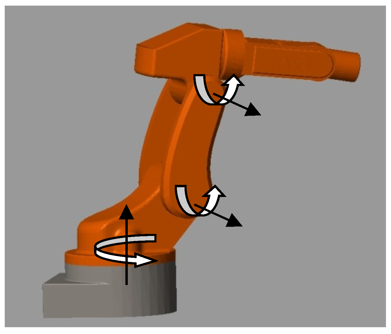
In this section, a simulation of the proposed fault-tolerant control algorithm for the 3-DOF manipulator shown in Figure 1 is described.

For this trajectory tracking simulation, the desired trajectories at each joint are given as

$$\{\begin{array}{l}{q}_{1d}=0.5\sin (t/2)\\ q_{2d}=0.3\sin (t)\\ q_{3d}=0.2\sin (t)\end{array}$$

(43)

The friction at each joint is assumed to be

$$\{\begin{array}{l}{F}_{1f}=0.2sgn({\dot{q}}_1)+0.3{\dot{q}}_1\\ F_{2f}=0.2sgn({\dot{q}}_2)+0.3{\dot{q}}_2\\ F_{3f}=0.2sgn({\dot{q}}_3)+0.3{\dot{q}}_3\end{array}$$

(44)

5.1. Simulation 1

In this part, the parameter selection of the extended state observer as seen in Equation (10) is explained. The total torque function at each joint is assumed to be

$$\{\begin{array}{l}{\tau }_1^t={\tau }_1\\ {\tau }_2^t=(1-{\rho }_2(t)){\tau }_2+f_2(t)t>5\\ {\tau }_3^t={\tau }_3\end{array}$$

(45)

where for loss of effectiveness, ${\rho }_2(t)=0.4\sin (\pi t)$, and a fault function $f_2(t)=60\sin (\pi t/2)$.

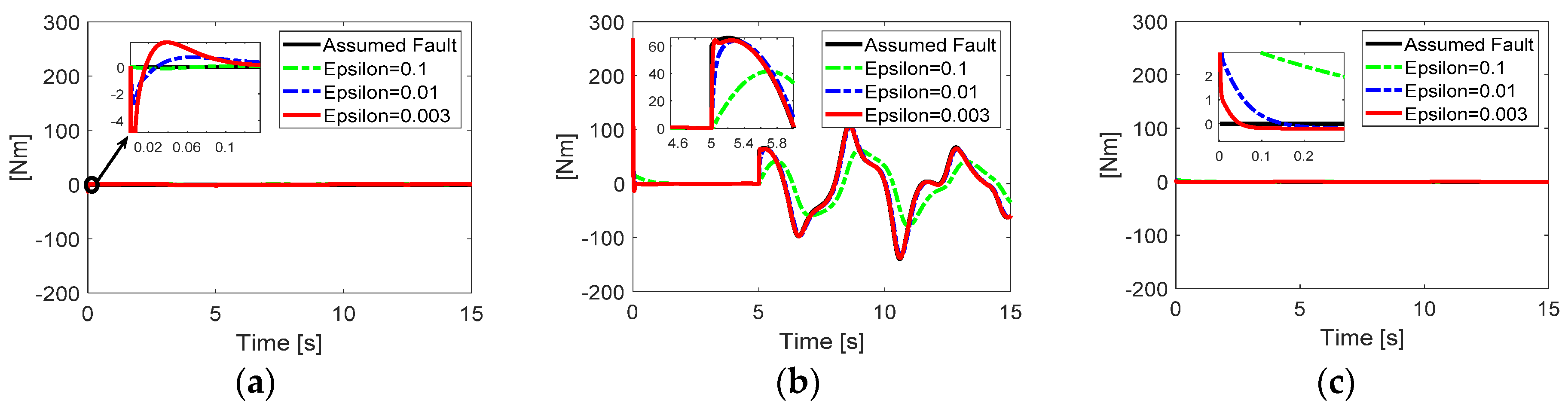
For the extended state observer of Equation (10), the four parameters such as ${\alpha }_1,{\alpha }_2,{\alpha }_3$ and $\epsilon$ should be suitably selected. The turning parameters in the set of ${\alpha }_1,{\alpha }_2,{\alpha }_3$ that should satisfy the Hurwitz condition are quite related to the qualities of the observer such as the accuracy and peaking values. From this consideration, the turning parameters were set as ${\alpha }_1=8,{\alpha }_2=28,{\alpha }_3=7$. For $\epsilon$, Equation (17) shows that the value of $\epsilon$ highly affects the behavior of the observer convergence. Therefore, three different values of $\epsilon =0.1, 0.01$, and $0.001$ were considered in this simulation. In Figure 2b, it can be seen that the peaking value highly defends the selection of $\epsilon$. The smaller value of $\epsilon$ causes faster convergence, but the high magnitude peaking value in the fault estimation. As a trade-off between the convergence and the peaking value, $\epsilon =0.01$ was selected.

5.2. Simulation 2

For comparison, a passive fault tolerant control with conventional sliding mode control (PFTC-SMC) and active fault-tolerant control with conventional sliding mode control (AFTC-SMC) were considered, in addition to the proposed active fault-tolerant control with synchronous sliding mode control (AFTC-SSMC).

The parameters of the observer were chosen as in Section 5.1. The AFTC-SMC is given as

$${\tau }_{AFTC\text{-}SMC}={\tau }_0+{\tau }_{smc}+{\tau }_{ob}$$

(46)

where ${\tau }_0=\mathbf{M}(q)({\ddot{q}}_d+c\dot{e})+\mathbf{H}(q,\dot{q})$, ${\tau }_{smc}=k_1\mathrm{sgn}(s)+k_{2}s$ and ${\tau }_{ob}=-\mathbf{M}(q)\stackrel{⌢}{\varphi }$, in which the sliding mode surface is selected as

$$s=\dot{e}+ce$$

(47)

The parameters in AFTC-SMC were suitably chosen as $c=diag(7;7;7),k_1=diag(220;220;220)$, and $k_2=diag(250;250;250)$. The PFTC-SMC is given as

$${\tau }_{PFTC\text{-}SMC}=\mathbf{M}(q)({\ddot{q}}_d+c\dot{e})+\mathbf{H}(q,\dot{q})+k_1\mathrm{sgn}(s)+k_{2}s$$

(48)

The parameters in PFTC-SMC were suitably chosen as $c=diag(7;7;7),k_1=diag(220;220;220)$ and $k_2=diag(250;250;250)$. The parameters of AFTC-SSMC were suitably chosen as $c=diag(7;7;7),$ $\alpha =diag(20;20;20),\kappa =diag(0.5;0.5;0.5),$$k_1=diag(220;220;220),k_2=diag(250;250;250),$ and $k_3=diag(30,30,30)$.

To avoid chattering, the signum function in Equations (25), (46), and (48) are replaced with the saturation function,

$$sat(s)=\{\begin{array}{ll}sgn(s)& if\left|s\right|\ge \lambda \\ \frac{s}{\lambda }& if\left|s\right|<\lambda \end{array}$$

(49)

where $\lambda =1.7$.

In this case, a failure occurs only at a single joint. The total torque function at each joint is assumed to be

$$\{\begin{array}{l}{\tau }_1^t={\tau }_1\\ {\tau }_2^t=(1-{\rho }_2(t)){\tau }_2+f_2(t)t>5\\ {\tau }_3^t={\tau }_3\end{array}$$

(50)

where ${\rho }_2(t)=0.4\sin (\pi t)$ and $f_2(t)=60\sin (\pi t/2)$.

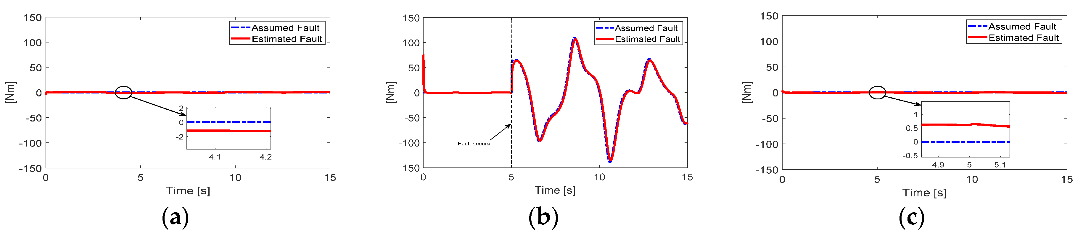
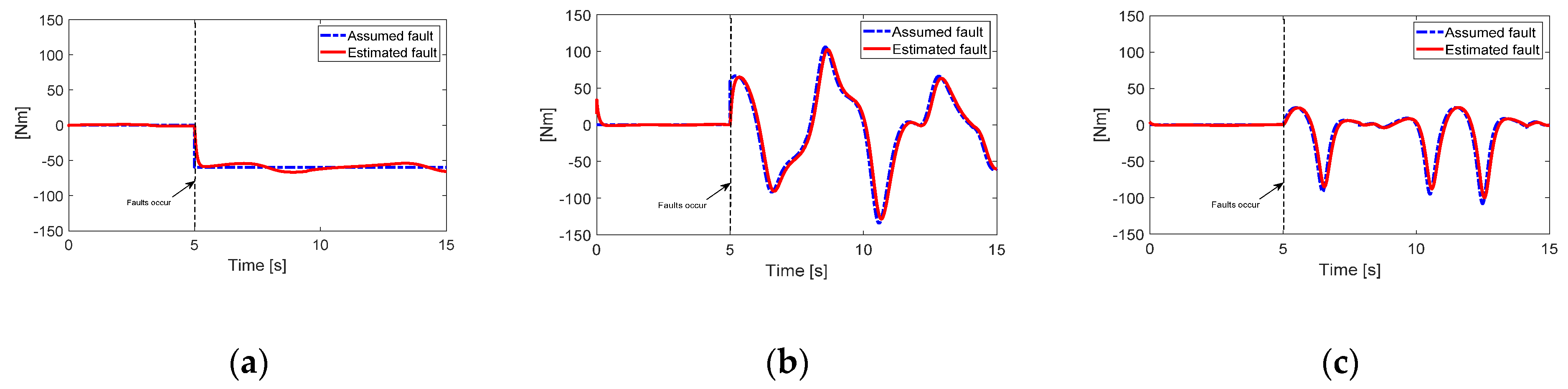
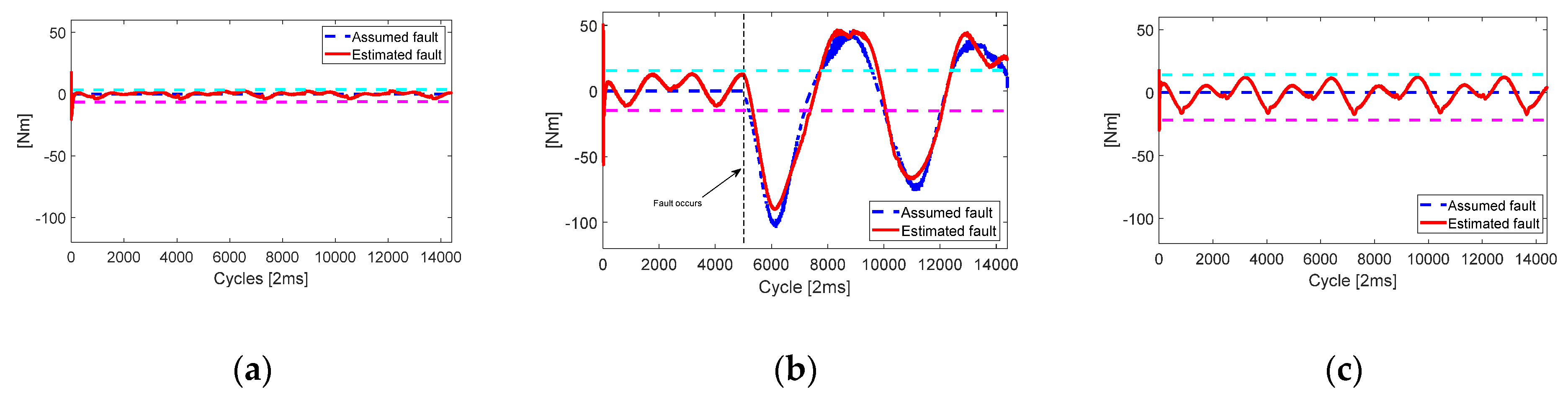
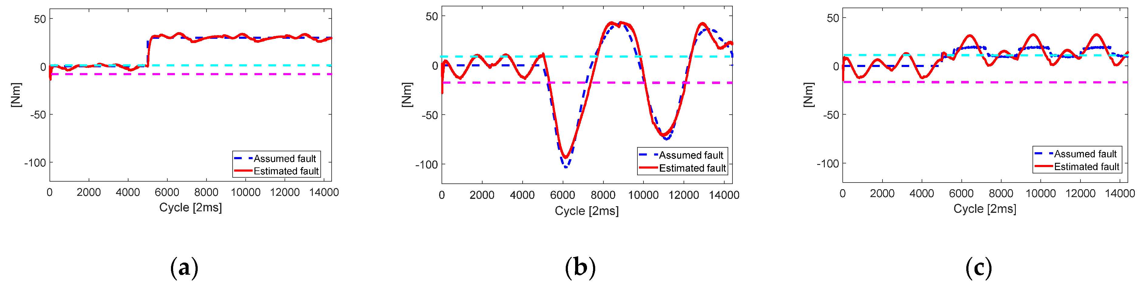
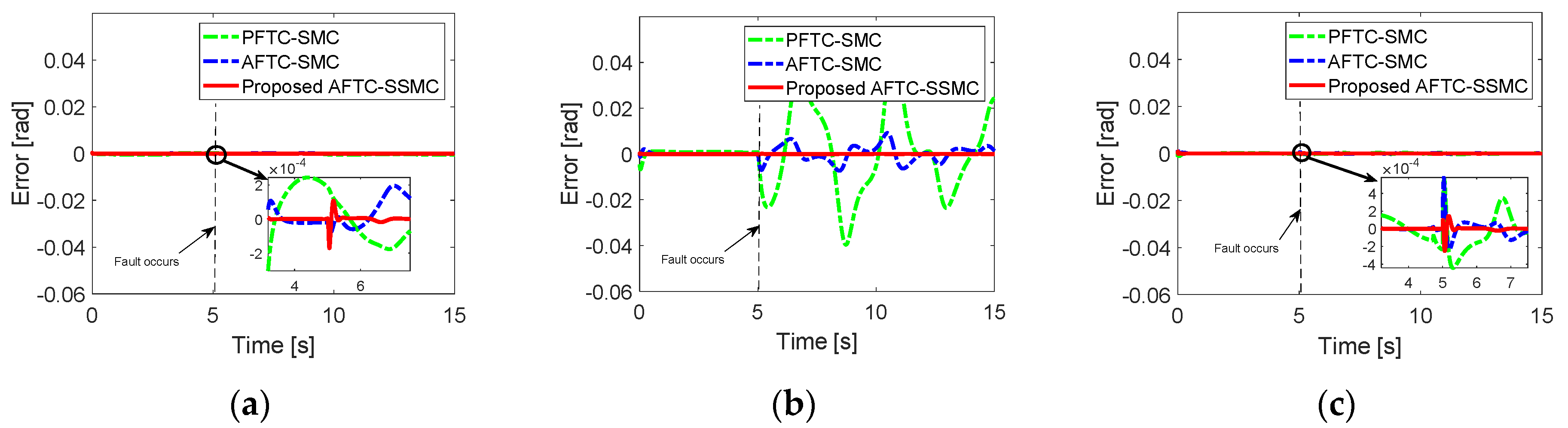
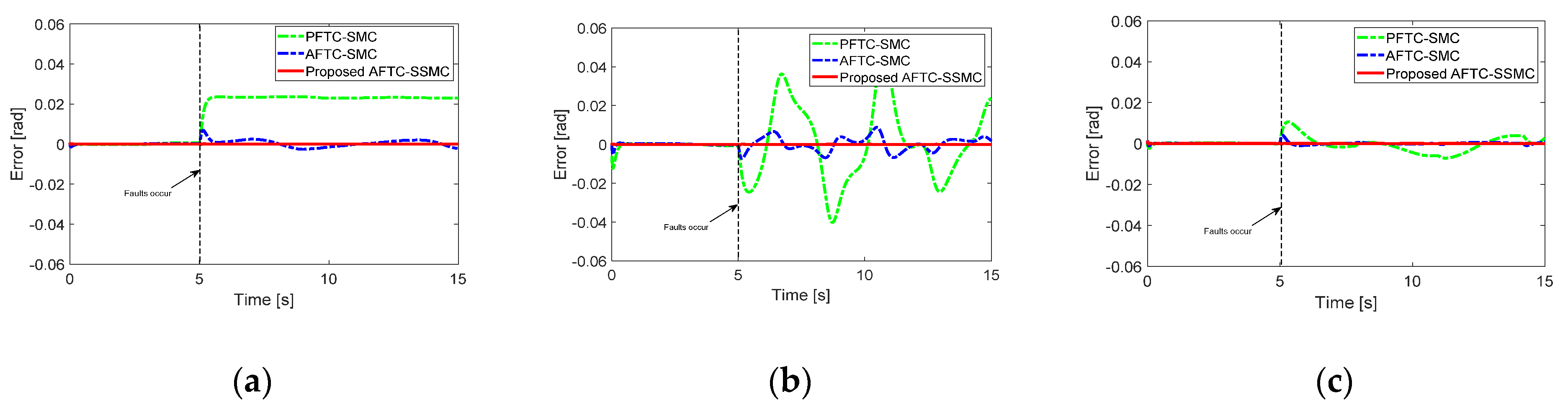
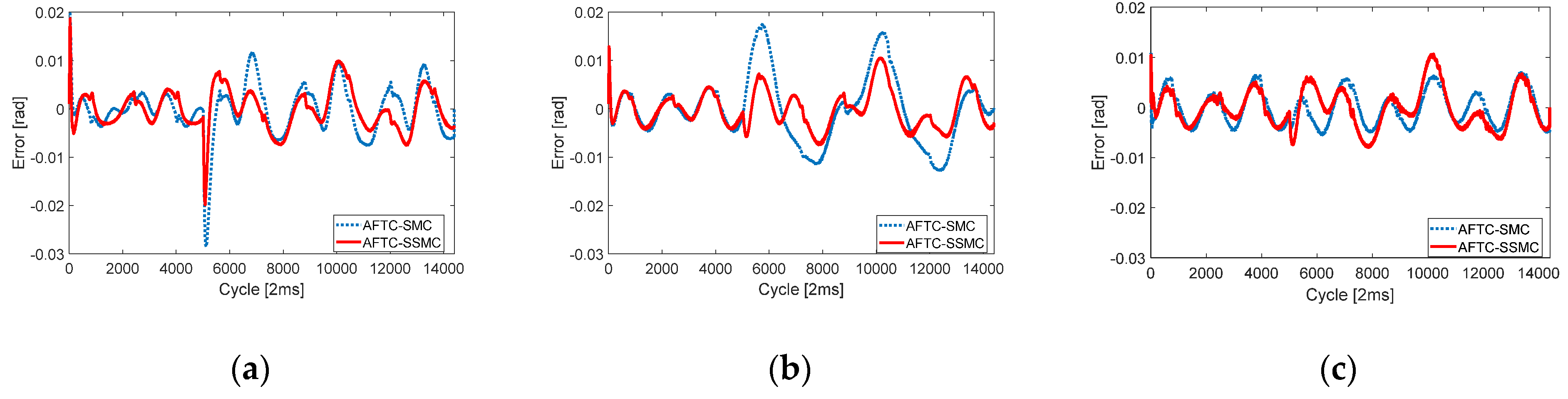
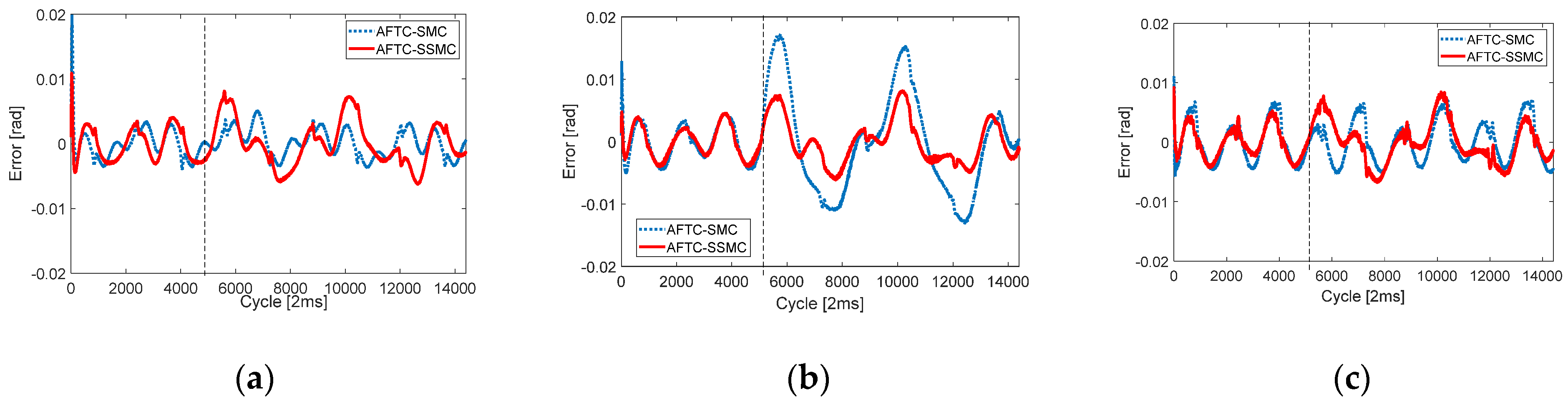
In Figure 3b, the single fault occurs at Joint 2 after five seconds. Figure 3 shows the fault estimation algorithm given in Equation (10) seems to be working well even though its estimation error still exists on the order of 1/100 of the fault magnitude. In Figure 4, without fault estimation, PFTC-SMC cannot guarantee the performance after the fault occurs. Unlike PFTC, the joint position errors of AFTC-SMC and proposed AFTC-SSMC look very different, but they were all on the order of 10⁻³, so that the overall trajectory tracking performance of the two control algorithms can be said to be acceptable in this simulation. However, it can be seen that the proposed AFTC-SSMC has very high accuracy after a fault occurs. This fault-tolerant capability can be said to come from the synchronous SMC. Each joint error is coupled and constrained due to the synchronization errors and the newly defined synchronous sliding surface.

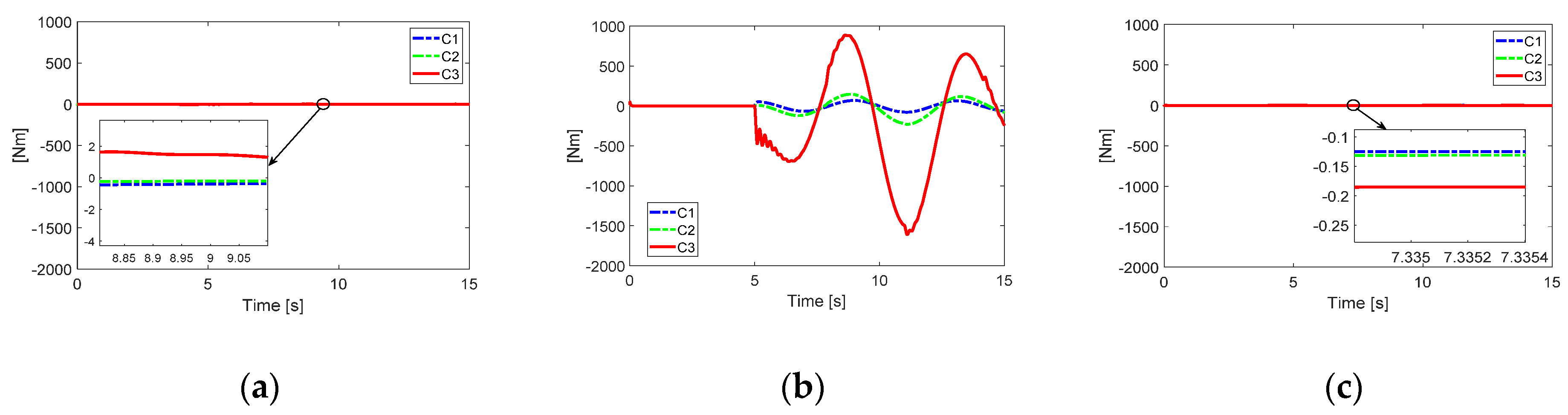
5.3. Simulation 3

In this part, the effect of the actuator loss effectiveness factor to the proposed fault tolerant control is discussed. The assumed fault is given as

$$\{\begin{array}{l}{\tau }_1^t={\tau }_1\\ {\tau }_2^t=(1-{\rho }_2(t)){\tau }_2+f_2(t)t>5\\ {\tau }_3^t={\tau }_3\end{array}$$

(51)

where the fault function of $f_2(t)=60\sin (\pi t/2)$ and ${\rho }_2(t)$ with the different values such as C1: ${\rho }_2(t)=0.1$, C2: ${\rho }_2(t)=0.5$, C3: ${\rho }_2(t)=0.9$. The selected parameters of the observer are in Section 5.2.

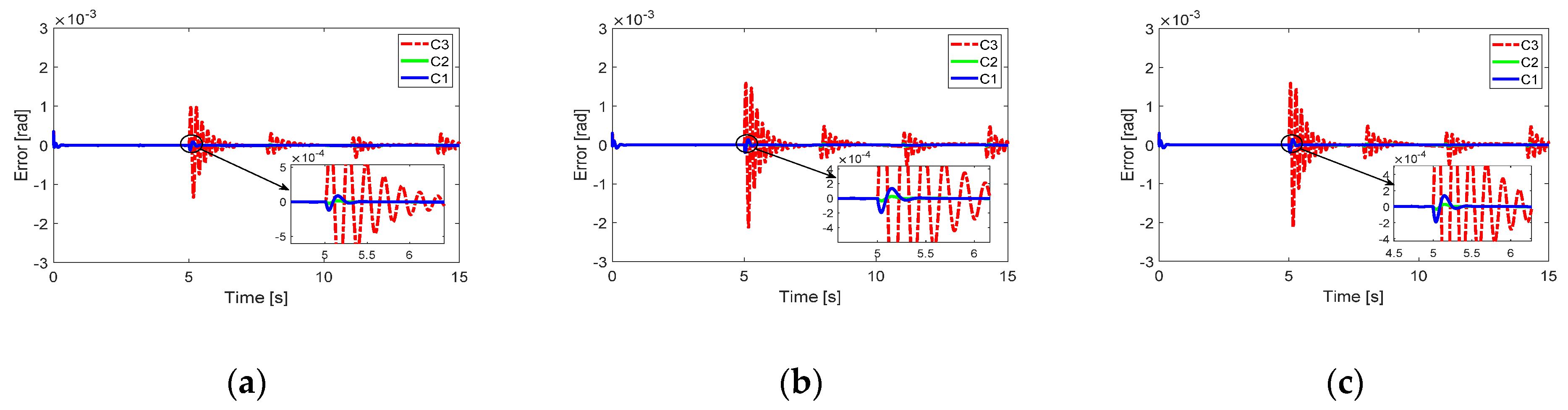
Even though the total fault function has a large magnitude with ${\rho }_2(t)$ of 0.9 as seen in Figure 5b, each joint error was still less than the value of ${10}^{-3}$ in Figure 6. Therefore, it can be said that the proposed fault tolerant control can have the capability to show acceptable performances, even in the case of a high value of ${\rho }_2(t)$.

5.4. Simulation 4

To test the robustness of the fault-tolerant characteristics of the proposed algorithm, simulations with multiple faults were performed with the three control algorithms Equations (25), (46) and (48), for which the parameters were selected in Section 5.2. Multiple faults/failure functions were assumed to be

$$\{\begin{array}{l}{\tau }_1^t={\tau }_1+f_1(t)\hspace{1em}t>5\\ {\tau }_2^t=(1-{\rho }_2(t)){\tau }_2+f_2(t)\hspace{1em}t>5\\ {\tau }_3^t=(1-{\rho }_3(t)){\tau }_3\hspace{1em}t>5\end{array}$$

(52)

where $f_1(t)=60$, ${\rho }_2(t)=0.4\sin (\pi t)$, $f_2(t)=60\sin (\pi t/2)$, and ${\rho }_3(t)=0.7\sin (\pi t)$.

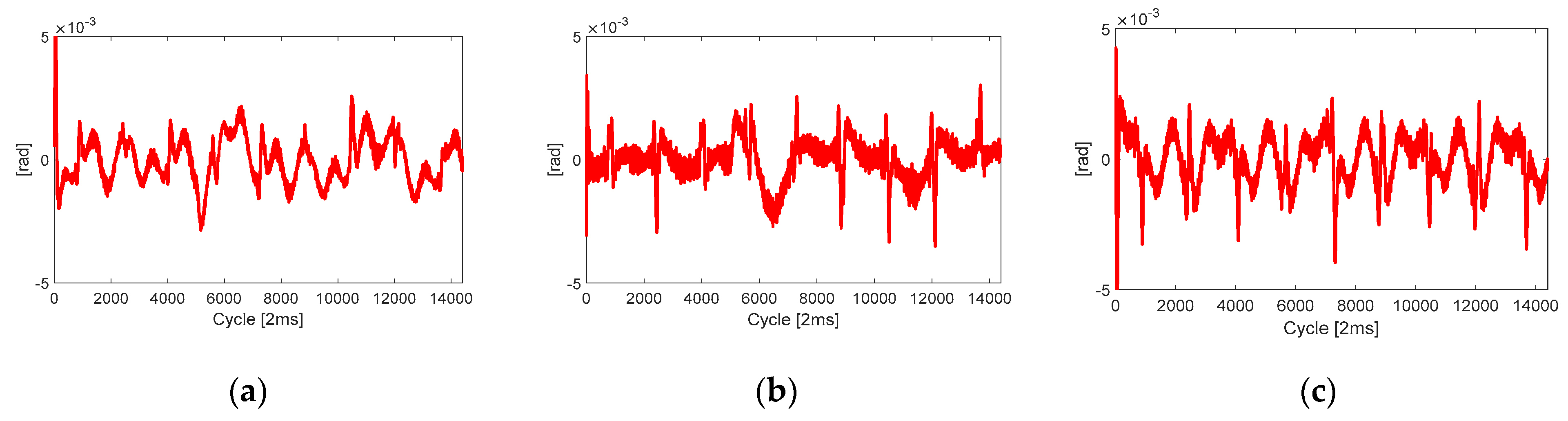
In Figure 7, the estimation results with multiple joint faults have been shown. Multiple faults simultaneously occurring at each joint seemed to burden the control system more than a single fault did. However, the proposed algorithm still resulted in smaller position-tracking errors than the conventional algorithm, demonstrating fault-tolerant characteristics, as seen in Figure 8.

Remark 1.

As mentioned in Section 1, the accuracy of fault estimation highly affects the performance of AFTCs, so Simulation 1 discussed the design of ESO. As a trade-off between the convergence and the peaking value of estimation results, the parameters of the observer were selected by using a trial–error technique, as shown in the Simulation 1 results. In Simulations 2, 3, and 4, the outperformance of the proposed controller was presented by the tracking trajectory error results. In Simulation 3, the robustness of the proposed controller was described with a high magnitude of fault. In this case, PFTC-SMC and AFTC-SMC could not guarantee stability of the system. However, the proposed AFTC-SSMC could keep the system stable and showed acceptable performance results with the tracking trajectory error inside${10}^{-3}$rad. In Simulations 2 and 4, single and multiple faults were presented. Compared with the two fault-tolerant controllers without the consideration of the synchronization error, the proposed controller can reduce the picking phenomenon due to the simultaneous approach to zero at each joint of the synchronization technique. This characteristic of synchronization control can act to prevent the slow response of AFTCs.

6. Experimental Results

In this section, the real implementation of fault-tolerant control with AFTC-SMC and the proposed AFTC-SSMC is described, and the experimental results were compared and discussed in the case of both single and the multiple joint faults.

6.1. Experimental Setup

The experimental setup is shown in Figure 9 with a 3-DOF FARA-AT2 robot manipulator. This robot manipulator has 6-DOF, but for these experiments joints 4, 5, and 6 were blocked. The 3-DOF FARA-AT2 robot had a CSMP series motor at each joint, and aCSMP-02BB driver was used for Joints 1 and 2 while the CSMP-01BB driver was used for Joint 3. The gear box at each joint is 120:1, 120:1, 100:1 at Joints 1, 2, and 3, respectively. The encoder at each joint was a 2048 line count incremental encoder. The controller ran on Labview-FPGA NI-PXI-8110 and NI-PXI-7842R PXI cards with the frequency control set at 500 Hz. NI-PXI-8110 was run on a Windows operating system.

The desired trajectory at each joint is given as

$$q_i(t)=\frac{\pi }{6}\sin (\frac{\pi t}{1600})\hspace{1em}(i=1,2,3)$$

(53)

6.2. Experimental Design

To reduce the high-frequency chattering of fault estimation of $\stackrel{⌢}{\varphi }$ in Equation (10) before it is used in the AFTC scheme, a simple low-pass filter was designed as

$${\stackrel{⌢}{\varphi }}_k^{filted}=(1-\upsilon ){\stackrel{⌢}{\varphi }}_{k-1}^{filted}+\upsilon {\stackrel{⌢}{\varphi }}_k$$

(54)

where ${\stackrel{⌢}{\varphi }}_k^{filted}$ and ${\stackrel{⌢}{\varphi }}_k$ are the output and input, respectively, of the low-pass filter at the $k^{th}$ step. The low-pass filter as seen in the next subsection allows the signal from the fault estimation (FE) to become smoother and is suitably applied to the AFTC schemes. However, the FE also increases the time delay of the feedback to the controller. To ensure that the smoothness and time delay are acceptable, $\upsilon =0.05$ was selected.

The related parameters of the FE in Equation (10) can be suitably selected as ${\alpha }_1=2,{\alpha }_2=3,{\alpha }_3=0.3$, and $\epsilon =0.01$.

The parameters of AFTC-SMC (Equation (46)) were suitably selected as $c=diag(3;3;3),k_1=diag(50;110;90)$, and $k_2=diag(50;100;90)$.

The parameters of the proposed AFTC-SSMC (Equation (25)) were suitably chosen as $c=diag(3;3;3),$$\alpha =diag(3;3;3),\kappa =diag(1.5;1.5;1.5),$$k_1=diag(50;110;90),k_2=diag(50;100;90),$$k_3=diag(30,30,30)$, and the $sign$ function in the control law in Equation (46) and the AFTC-SSMC was replaced by the saturation function

$$sat=\{\begin{array}{ll}sgn(s)& ifs>\lambda \\ s/\lambda & ifs\le \lambda \end{array}$$

where $\lambda =1.6$.

6.3. Experimental Results

6.3.1. Single Fault

In this experiment, the fault occurred only at a single joint after 10 s. The desired fault function includes bias, and the fault is assumed to be

$$\{\begin{array}{l}{\tau }_1^t={\tau }_1\\ {\tau }_2^t=(1-{\rho }_2(t)){\tau }_2+f_2(t)t>5000\\ {\tau }_3^t={\tau }_3\end{array}$$

(55)

where ${\rho }_2(t)=0.4\sin (\pi t/2400)$ and $f_2(t)=-60\sin (\pi t/2400)$.

The results are shown in Figure 10, Figure 11 and Figure 12. First, in Figure 10, the fault estimation is presented where the dashed aqua and pink lines are the upper and lower thresholds, respectively. The estimation results of the uncertainties and disturbance were within the thresholds for Joints 1 and 3, and for Joint 2 before the fault occurred. In contrast to the simulation results, the fault estimation results were not close to 0 before the fault occurred because in practice, relatively high value for the uncertainties and disturbances always exist. Therefore, using such thresholds is a good method for monitoring when faults occur in real applications. As shown in Figure 10, the extended state observer estimated the fault well. In Figure 11, the tracking error performance at each joint is shown. Before the fault occurred, the tracking trajectory of the proposed AFTC had no advantage over the AFTC with conventional sliding mode control. However, after the fault occurred, the advantages of the proposed AFTC were observed; the error at Joint 2 with AFTC-SSMC was smaller than that of AFTC-SMC, and the joint error was approximately 0.005 rad when the fault occurred. This means that the proposed controller has the ability to prevent tracking errors from getting larger due to a fault, and thus averting a critical condition (Figure 11b); the Joint 2 error of the AFTC-SSMC was reduced when compared to that of the AFTC-SMC after faults. However, the Joints 1 and 3 errors of AFTC-SSMC were slightly increased compared with those of AFTC-SMC after faults (Figure 11a,c). This is probably due to the synchronization techniques, which tend to drive all joint errors to be comparable. The proposed synchronous control seems well-suited for fault tolerant control. In addition, the synchronization joint errors theoretically approached zero, and as shown in Figure 12, they remained less than ~0.0025 rad in this experiment.

6.3.2. Multiple Faults

The effectiveness of the proposed fault-tolerant control in the case of multiple faults was also investigated. The desired faults occurred after 10 sand are assumed to be

$$\{\begin{array}{l}{\tau }_1^t={\tau }_1+f_1(t)\hspace{1em}t>5000\\ {\tau }_2^t=(1-{\mathsf{\rho }}_2(t)){\tau }_2+f_2(t)\hspace{1em}t>5000\\ {\tau }_3^t=(1{-\mathsf{\rho }}_3(t)){\tau }_3\hspace{1em}t>5000\end{array}$$

(56)

where $f_1(t)=30$, ${\rho }_2(t)=0.4\sin (\pi t/2400)$, $f_2(t)=-60\sin (\pi t/2400)$, and ${\rho }_3(t)=-0.7$.

The overall results of this experiment are similar to the previous results from the simulations and the single fault experiments. The fault estimation capability is still at the same level as that of the single fault case, as seen in Figure 13. The trajectory tracking performances of the two algorithms can be said to have behaviors similar to those seen in Figure 14. AFTC-SSMC showed the smaller trajectory tracking errors, especially after the faults occurred at 10 s, demonstrating the fault-tolerant characteristics, even in this multiple faults case. In Figure 14a,b, it can be seen that the picking phenomenon due to the slow response of the AFTC strategy was reduced by using the synchronization technique. And the synchronization joint errors were shown in Figure 15.

Remark 2.

In this section, the experimental results were discussed. The resulting tracking trajectory errors were shown with single and multiple faults. In a real system, the uncertainties and disturbances have a higher magnitude than that of the simulation environment. Due to the limitation of selection parameters in a real system, the robot system with PFTC-SMC failed when multiple faults occurred. Therefore, in these experimental results, only the results of AFTC-SMC and the proposed AFTC-SSMC were presented. As mentioned in Section 1, the synchronization technique does not show effectiveness in an open-chain system such as a serial robot manipulator. Therefore, before a fault occurs, both controllers have a similar accuracy level. After a fault occurs, due to the slow response of AFTCs, the controller without the consideration of the synchronization error showed a high picking value at the joint fault. The proposed controller with a constraint within the synchronization technique quickly responded to the occurrence of faults before the system had the feed-back information from fault estimation. Hence, AFTC-SSMC showed better performance than AFTC-SMC. However, in a real system, due to the limitation of adjustment controller parameters, the error at joints without faults were slightly increased when compared with those of AFTC-SMC by the synchronization technique. This characteristic may be a disadvantage of this proposed controller. However, the AFTC-SSMC still showed an acceptable performance at these actuators.

7. Conclusions

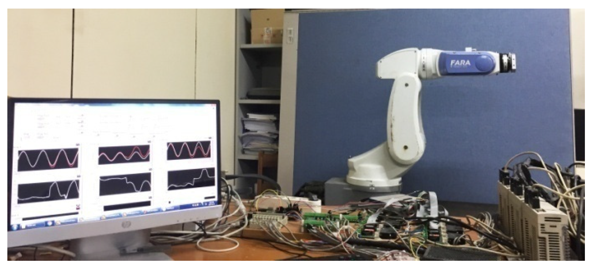
In this paper, an active fault-tolerant control for a robot manipulator based on synchronous sliding mode was proposed. To verify its effectiveness, experimental implementation of the proposed control algorithm for a three degree-of-freedom FARA-AT2 robot were carried out and compared with the active fault-tolerant control with conventional sliding mode control in the both single and multiple fault cases. The results indicate that the active fault-tolerant control with synchronous sliding mode control has better fault-tolerant capability and results in better trajectory tracking performance when compared to the active fault-tolerant control with conventional sliding mode control algorithms. This fault-tolerant capability comes from synchronous sliding mode control, because each joint error is coupled and constrained due to the synchronization errors and newly defined synchronous sliding surface. Future work includes the optimal tuning of synchronization parameters by following some methods (e.g., the genetic algorithm, neural network technique, etc.) In addition, the synchronization technique will be applied to finite-time control such as terminal sliding mode control, non-singular terminal sliding mode control, and so on, in fault-tolerant control for a serial robot manipulator.