Article

A Deep Regression Model with Low-Dimensional Feature Extraction for Multi-Parameter Manufacturing Quality Prediction

1
School of Mechanical Engineering, Dongguan University of Technology, Dongguan 523808, China
2
Centro de Electrónica, Optoelectronica e Telecomunicações, Universidade do Algarve, 8005139 Faro, Portugal
*
Author to whom correspondence should be addressed.
Appl. Sci. 2020, 10(7), 2522; https://doi.org/10.3390/app10072522
Submission received: 28 February 2020 / Revised: 26 March 2020 / Accepted: 2 April 2020 / Published: 6 April 2020

Abstract

:
Manufacturing quality prediction can be used to design better parameters at an earlier production stage. However, in complex manufacturing processes, prediction performance is affected by multi-parameter inputs. To address this issue, a deep regression framework based on manifold learning (MDRN) is proposed in this paper. The multi-parameter inputs (i.e., high-dimensional information) were firstly analyzed using manifold learning (ML), which is an effective nonlinear technique for low-dimensional feature extraction that can enhance the representation of multi-parameter inputs and reduce calculation burdens. The features obtained through the ML were then learned by a deep learning architecture (DL). It can learn sufficient features of the pattern between manufacturing quality and the low-dimensional information in an unsupervised framework, which has been proven to be effective in many fields. Finally, the learned features were inputted into the regression network, and manufacturing quality predictions were made. One type (two cases) of machinery parts manufacturing system was investigated in order to estimate the performance of the proposed MDRN with three comparisons. The experiments showed that the MDRN overwhelmed all the peer methods in terms of mean absolute percentage error, root-mean-square error, and threshold statistics. Based on these results, we conclude that integrating the ML technique for dimension reduction and the DL technique for feature extraction can improve multi-parameter manufacturing quality predictions.

1. Introduction

High manufacturing quality grants manufacturers a competitive edge. Modern manufacturing processes exhibit new characteristics, such as multi-stage and multi-parameter inputs, both of which influence quality. High-quality products tend to stem from the design of appropriate manufacturing parameters. Hence, designing favorable parameters hinges on predicting manufacturing quality at an early production stage, which provides reference for set high-quality products at lower costs.
Several approaches and methods have been adopted to predict manufacturing quality. Statistical quality control [1], a traditional method, has been widely used to assess the quality and performance of manufacturing processes. Based on this method, other techniques have been developed, e.g., linear regression [2,3], nonlinear regression [4], inference learning [5], fuzzy theory [6], and graph theory [7]. These approaches have successfully been applied to manufacturing quality prediction, but only in situations in which the factors (e.g., materials, equipment, and technological parameters) maintain a certain level of stability. This narrow application limits the use of these methods. In particular, these methods act as a bottleneck when handling multi-parameter manufacturing. Recently, the development of computer technologies, such as artificial intelligence, has caught the attention of researchers, because of their minimal information requirements, which do not need to take into account the manufacturing processes [8,9,10,11]. Artificial neural networks (ANNs) are among the most famous representations, alongside self-organizing neural network [12], back propagation neural network (BPNN) [13], radial basis function neural network [14], and probability neural network [15]. As it is affected by multi-parameter inputs from the multi-stage manufacturing processes, the ANN modeling exhibits feature learning difficulties and network calculation complexities. Therefore, to ensure prediction accuracy, it is imperative to develop and apply new techniques using multivariate analysis, as well as an intensive network to enable feature extraction and learning.
Recently, various multivariate analysis approaches have been widely applied to manufacturing processes for different industries, for example, principal component analysis (PCA) [16], linear discriminant analysis [17], rough-set theory [18], independent component analysis [19], and feature reinforcement approach [20]. However, these approaches have only affected the datasets of linear structures and gauss distributions; they are not suitable for use with real data with nonlinear features. To overcome this problem, manifold learning (ML), seeking to find a low-dimensional parameterization of high-dimensional data, has been proposed [21]. As a result of its nonlinear computational efficiency, global optimality, and asymptotic convergence guarantees, ML has also been employed in applications such as dimension reduction and feature extraction [22,23,24]. These studies indicated that the ML technique is capable of better restoring intrinsic dimension from high-dimensional data. Thus, it reduces the multi-parameter disturbances in feature learning.
To enhance the feature learning of ANN, a deep learning (DL) technique has been proposed [25,26], and, combined with the ANN framework, forms a deep neural network (DNN). Unlike a traditional network (shallow learning), the foundation of a DNN is its hierarchy; that is, the information representation is delivered from lower to higher levels, which makes the higher levels more abstract and nonlinear. Through representation by the hierarchical levels, the “deeper” feature of the multi-parameter inputs and the manufacturing quality can be sufficiently fitted by the regression models [27]. Therefore, the DNN has been widely used in applications such as classification [28] and time series forecasting [29]. The DL techniques are also utilized in the manufacturing field [30,31,32]. However, to our knowledge, there have been few attempts to employ the DL architecture for manufacturing quality prediction.
By considering the superiority performance of ML in reducing the dimensions of multi-parameter inputs, and DNN for learning sophisticated features of manufacturing processes, a manifold learning-based deep regression network (MDRN) is proposed for the multi-parameter manufacturing quality prediction conducted in this paper. The contribution of this work is integrated with DNN for reinforcing feature representation via ML for reducing redundant information, thus reducing the modeling complexity and improving the prediction performance. The proposed MDRN model was realized in the following three stages: (i) the ML technique was firstly used to learn the intrinsic coupling features of the relevant manufacturing multi-parameter inputs through dimension reduction, (ii) the DL method was then applied to dig the features of the pattern with the manufacturing quality and the low-dimensional information achieved by ML, and (iii) the ANN for regression was finally employed to model the deep representations generated by the DL and achieve the manufacturing quality predictions. Stage (ii) and stage (iii) were integrated into the deep regression network (DRN). To investigate the prediction capacity of the proposed model, a machinery parts manufacturing system with multi-parameter inputs was utilized for modeling and validation. Comparisons with other peer models were also performed.
The rest of the paper is organized as follows. Section 2 presents the manifold learning, deep regression network, and proposed model, respectively. Section 3 describes the application of the addressed model. Section 4 gives the results with relevant discussion. Section 5 concludes this work.

2. Methodologies

2.1. Manifold Learning for Low-Dimensional Feature Extraction

As introduced in Section 1, ML, aiming to explore the intrinsic geometry of dataset, has proven its effectiveness in nonlinear reduction dimensionality. Recently, various ML methods have been developed, e.g., isometric mapping (Isomap) [21], locally linear embedding (LLE) [33], Laplacian eigenmaps (LE) [34], Hessian eigenmaps (HE) [35], and local tangent space alignment (LTSA) [36]. Compared with these approaches, the computation of the Isomap is the simplest, with only one parameter to be determined. Hence, the Isomap was applied for the manufacturing multi-parameter analysis in this paper. Below the steps of the algorithm are described as follows [21]:
Let X = [x1, x2, …, xn] denotes the manufacturing multi-parameter set with dimension n, and Y = [y1, y2, …, ym] denotes the low-dimensional space with dimension m.
Step 1. Construct the neighborhood relationships. When the Euclidean distance d(xi, xj) between xi and xj is closer than the radius ε, or xi is one of the K-nearest neighbors of xj, xi and xj can be regarded as neighbors.
Step 2. Compute the shortest distances. Define the graph, G, over all data points by connecting d(xi, xj). If xi and xj are neighbors, dG(xi, xj) = d(xi, xj), otherwise, dG(xi, xj) = ∞. Evaluate the geodesic distances, DG, between all pairs of data points by computing their shortest path distances, dG(xi, xj), using Floyd’s algorithm [37].
Step 3. Construct m-dimensional embedding. This step is realized through the classical multidimensional scaling method, as follows: Let λp be the p-th eigenvalue (in decreasing order) of the matrix τ(DG) = -HSH/2 (S is the matrix of squared distances Sij = [dG(xi, xj)]2, and H = I-(1/N)EET is the centering matrix, where I means unit matrix with N dimension (length of xi or xj), and E denotes the vector of all ones), and vpi is the i-th component of the p-th eigenvector. Then, set the p-th component of the m-dimensional coordinate vector yi = (λp vpi)0.5.
Based on the description above, the radius, ε, or the number of neighbors, K, is the only parameter in the Isomap algorithm. In this paper, the K-Isomap was applied for dimension reduction. To our knowledge, there is no general theory for determining the K (a common-used approach is empirical method). In addition, the instinct low dimension, m, was specified by the maximum likelihood estimator (MLE) [38].

2.2. Deep Regression Network for Manufacturing Quality Prediction

After achieving the low-dimensional information (Y), the DL technique was adopted to learn the essential features of the pattern with the low-dimensional information and the manufacturing quality.
As shown in Figure 1, the DNN is a stack of simple networks (an autoencoder (AE) in this paper [39], named AE-based DRN) with the following three steps [40]: (i) from the lowest to top layers (layer 1 to layer l, from left to right), generative unsupervised learning occurred layer-wise on the AE; (ii) from the top to lowest layers (layer l to layer 1), fine-tuning by a supervised learning method (back propagation algorithm) is used to tweak the parameter sets (w, b); and (iii) from the hidden (top) to the output layer, a regression network is formed using the pre-training parameter sets (w, b).
As Figure 1 illustrates, the AE model operates as follows. The purpose of the AE is to reconstruct inputs hl−1 (h0 = Y) into new representations, R = [r1, r2, …, rm], with a minimum reconstruction error, as follows:
R E ( h l 1 , R ) = m = 1 M [ h m l 1 log ( r m ) + ( 1 h m l 1 ) log ( 1 r m ) ]
To address this issue, the AE-based DRN is operated step by step for encoder, fe(.) (feature extraction function), and decoder, fd(.) (reconstruction function), until the optimal parameter sets (w, b) are achieved based on a minimal loss function (Equation (3)).
h l = f e ( h l 1 ) = S i g m ( w h l 1 + b ) ,   r = f d ( h l ) = S i g m ( w T h l + b T ) ,
where Sigm(.) means the sigmoid activation function. The minimal loss function is as follows:
L ( w , b ) = R E ( h l 1 , R ) .

2.3. Overview of the Proposed MDRN Approach

Having addressed the constituents separately, the present approach for the manufacturing quality prediction can be summarized as follows, and is illustrated by Figure 2.
Step 1. Collect multi-parameter X and the corresponding quality from each manufacturing batch.
Step 2. Perform the K-Isomap algorithm and get the low-dimensional information Y.
Step 3. Construct the DRN model and get the quality prediction.
(a) Construct the AE-based deep framework for the feature learning of Y, and get the parameter sets (w, b).
(b) Initialize the regression network with the parameter sets (w, b) pre-trained by (a), and model the relationships between Y and the corresponding quality.

3. Data Description and Evaluation Indexes

3.1. Dataset

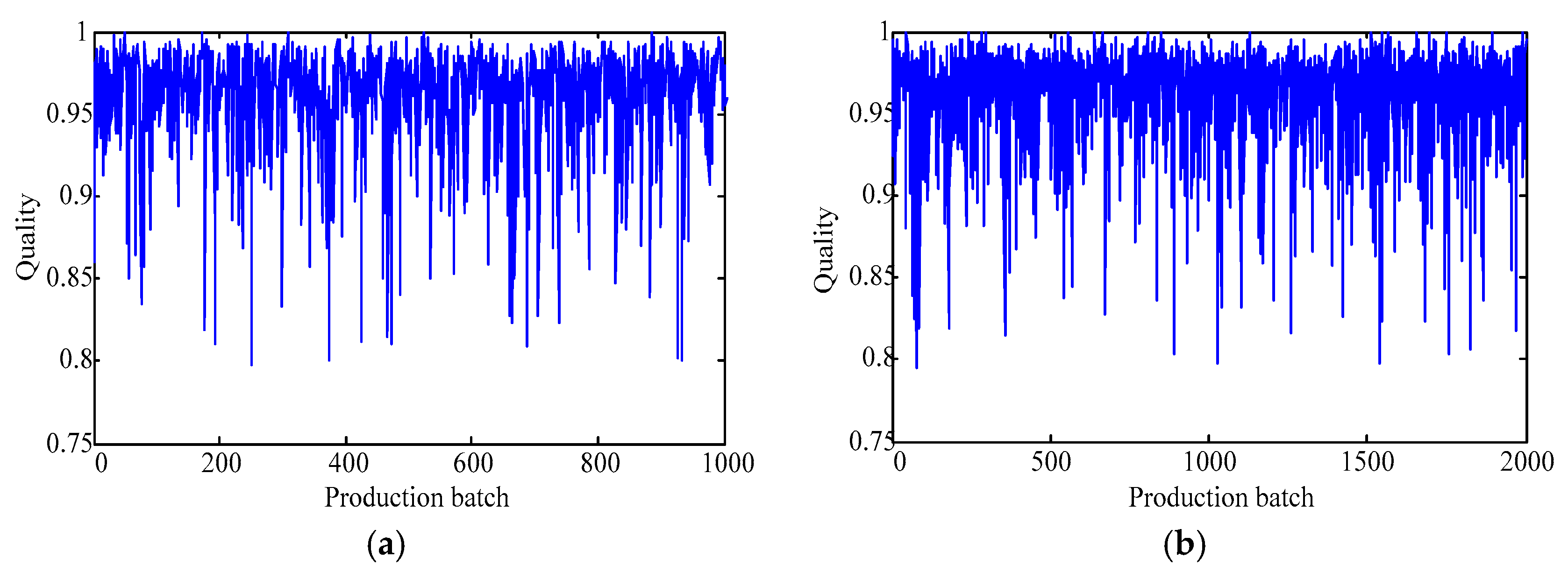
The data were collected from two manufacturing lines for the same product (machinery parts). The data were available from a competition about manufacturing quality control, which is organized by the Alibaba Company [41]. The data have the same technique parameters (i.e., 19 process parameters, shown in Table 1) with different settings; thus, the quality index (one key-quality index with range [0, 1], shown in Figure 3) exhibits diversity in different batches. Case 1 includes 1000 batches, with the total sample being (19 + 1) × 1000, and Case 2 includes 2000 batches, with the total sample being (19 + 1) × 2000. These data were divided into two categories, 90% for training and 10% for testing. Note that all the data were desensitized.

3.2. Model Development

In this subsection, the ingredients of the proposed model, that is, the K-Isomap and the DRN for the real manufacturing system are defined in detail. Note that all of the data are normalized into [0, 1]. Then, the experimental method is applied to construct the proposed MDRN model. The details of the model developments are listed in Table 2.

3.3. Performance Criteria

Three criteria are employed to assess the forecasting performances, namely: mean absolute percentage error (MAPE; %), root-mean-square error (RMSE; dimensionless value), and threshold statistics (TS; %). The definitions of three criteria are listed as follows:
M A P E = 100 B i = 1 B | o b i p r i o b i | ,   R M S E = i = 1 B ( o b i p r i ) 2 / B ,   T S a = n a B × 100 ,
where B is the length of the prediction; obi and pri represent the i-th observation and prediction, respectively; and na is the number of data predicted having relative error in forecasting less than a %. In this paper, TSa is calculated for three levels of 1%, 5%, and 10%.

4. Results and Discussion

4.1. Proposed MDRN Results

Firstly, take Case 1 as an example to introduce the modeling process in detail. As mentioned in the Methodologies section, the instinct dimension of the multi-parameter in the manufacturing system (Table 1) is firstly evaluated by the MLE, and the result is 3, i.e., m = 3. Then, the experiments of the model development are implemented based on Table 2, and the performance (MAPE) of the proposed MDRN model is shown in Figure 4.
For the Isomap algorithm, some statistical data are summarized, namely: K = 8, the range of the MAPE is between 2.444% and 2.639% (mean value 2.560%); K = 10, the range of the MAPE is between 2.345% and 2.686% (mean value 2.513%); K = 12, the range of the MAPE is between 1.943% and 2.624% (mean value 2.365%); and K = 14, the range of the MAPE is between 2.183% and 2.671% (mean value 2.429%). These results indicate that the prediction performance improves as K increases, but they also prove that a large value of K may lead to performance degradation. Therefore, K = 12 is an appropriate selection in this paper.
For the DRN model shown in Figure 4, the prediction performance of the deep structure is better (slight or significant) than that of the “shallow” framework (one hidden layer), except for a few special samples. In addition, the deep structures with different K values exhibit the diversity in deep representations, that is, when K = 8, the best deep structure is 50 × 50 with 2.444% (hidden layer l = 2, 50 nodes in each hidden layer); when K = 10, the best deep structure is 40 × 40 with 2.345% (hidden layer l = 2, 40 nodes in each hidden layer); when K = 12, the best deep structure is 30 × 30 with 1.943% (hidden layer l = 2, 30 nodes in each hidden layer); and when K = 14, the best deep structure is 10 × 10 with 2.183% (hidden layer l = 2, 30 nodes in each hidden layer). Therefore, the deep structure 30 × 30 with K = 12 was chosen as the optimal pattern for Case 1 prediction (marked as 3-30-30-1), and the results and residual analysis are plotted in Figure 5.
As Figure 5a shows, the prediction trends are, to some extent, in accordance with the measurement trends, but there are also some significant differences between the two values. As shown in Figure 5b, the residual errors cause some fluctuation in the testing processes within the range of [−0.1, 0.1]. There are only five prediction outliers in a triangle, because the interval around the residual errors does not contain zero. This implies that the five residual errors that are caused by the unfortunate fitting, and have a confidence interval of over 95%, accounted for 5% of the testing data. Furthermore, the quantitative evaluation results, MAPE = 1.943% and RMSE = 0.022, also exhibit a high accuracy. Hence, the thorough processes of the testing are successful, and the results are acceptable.
Following the modeling process of Case 1, the testing results of Case 2 are plotted in Figure 6. Note that the optimal MDRN model for Case 2 is constructed by m = 3, K = 14, and has a deep structure of 25 × 25 (hidden layer l = 2, with 25 nodes in each hidden layer), i.e., 3-25-25-1.
The results shown in Figure 6 can be summarized as follows: (1) The instinct dimension, m, is related to the data feature, not the length of data. The calculation result, that is, m = 3, is the same, because it uses the same type of manufacturing parameters (x1-x19). (2) Because of its deep feature learning capacity, the DRN with two hidden layers achieves better prediction results (MAPE = 1.861% and RMSE = 0.023) than that of the model with a single hidden layer. (3) There are eleven outliers (accounting for 5.5% of the testing data) in the residual error analysis, which illustrate that the MDRN approach has a stable ability for feature learning and regression, because of the 5% of outliers in the Case 1 prediction.
Table 3 summarizes the quantitative results in the training and the testing process for the robust analysis. From Table 3, one can find that all performances in both the training and testing processes are similar, indicating that the proposed model has a generalization ability and robustness. It is attributed to the “dropout”, which weakens the joint adaptability between neurons (that is, the parameters of the whole network neurons are only partially updated because of the different neurons eliminated each time).
According to the quantitative and qualitative analysis above, the proposed MDRN model, which combines the Isomap for multi-parameter reduction and the DRN for the relationship between the low-dimension information and manufacturing quality learning, predict the manufacturing quality within an acceptable margin of error. In addition, the performance of the model with three hidden layers is not greater than that of the model with two hidden layers. This phenomenon is different from the DL theory, in which the deeper the hidden layer is, the better the performance is. That is, the deep architecture is closely related to the internal features of the real data. Furthermore, the proposed model has a generalization ability and robustness. Therefore, suitable deep architecture and the lack of blind pursuit for more hidden layers can avoid computational burdens and enhance the prediction performance.

4.2. Comparison Results

To evaluate the prediction performance of the proposed model, three models are applied to the comparisons using the same dataset, i.e., the AE-based DRN, the BPNN, and least squares support vector regression (LSSVR). The BPNN with one hidden layer and the LSSVR with the kernel function (none hidden layer) are typical shallow learning frameworks in the peer work. All of the models have the same input–output structures (19 inputs and 1 output), and the hidden layer and hidden node (except for the LSSVR) are specified by the experimental method.
For the AE-based DRN, the experimental design is the same as the “DRN for manufacturing quality prediction” shown in Table 2. The optimal model structure is set as the hidden layer l = 2, with 25 nodes in each hidden layer for Case 1, and it is set as the hidden layer l = 2, with 25 nodes in each hidden layer for Case 2.
For the BPNN, an empirical formula is applied to determine the hidden node, i.e., h i d d e n   n o d e s = i n p u t n o d e s + o u t p u t n o d e s + b ( b [ 0 , 10 ] ) . Therefore, the optimal hidden node for Case 1 and Case 2 is calculated as 10 and 12, respectively, in terms of the MAPE. In addition, other main computing parameters are set to a learning rate of 0.05 and a goal of 0.0001 for 200 iterations.
For the LSSVR, there are two parameters, i.e., kernel width and penalty coefficient [9], that are determined using the ten-fold cross-validation method in this paper. Hence, the optimal parameters are set as (25.016 and 9.565) for Case 1 and (20.525 and 10.410) for Case 2.
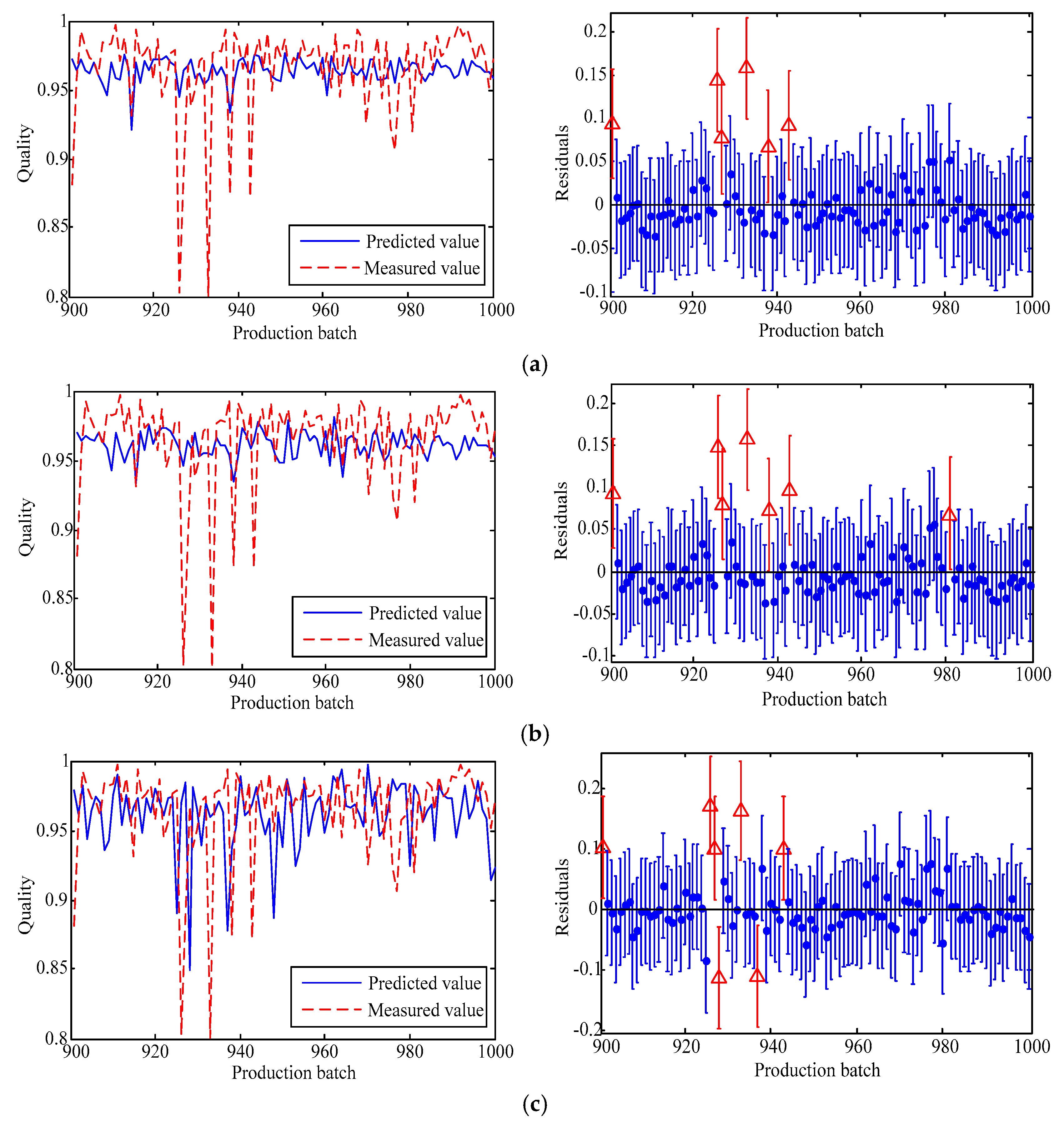
The prediction results for the two cases using the three models are displayed in Figure 7 and Figure 8, seperately.
Figure 7 reveals the following: (1) There are some unsatisfactory prediction results in the three models for Case 1, which illustrate that the performance is not related to the multi-parameter inputs; rather, it is related to the input feature. Compared with Figure 5, the three comparison models, which consider 19 parameters, exhibit a lower prediction performance. Specifically, there are six (accounting for 6% in the test data) outliers in the AE-based DRN, and seven (accounting for 7%) outliers in both the LSSVR and the BPNN. (2) Deep architecture is superior in performance to feature learning. That is, the performance of the proposed model and the AE-based DRN is better than that of the LSSVR and the BPNN in terms of the number of outliers. Cumulatively, the MDRN model has the best performance for Case 1 among these comparison models, attributed to multi-parameter reduction and deep feature representation, both of which reduce the invalid information interference and improve the prediction capacity.
As Figure 8 illustrates, the fluctuations in the three models also exhibit diversity, and are caught in the mutations. The residual analysis shows evidence of 10 outliers (accounting for 5%) in the AE-based DRN and the LSSVR model, and 12 outliers (accounting for 6%) in the BPNN. Compared with Figure 6, the performance of the MDRN model is in a second place with 11 outliers. This result of Case 2 differs with that of Case 1. Therefore, to evaluate the performance of these models, quantitative evaluations are also investigated, and the results are summarized in Table 3.
As shown in Table 4, the statistical indexes of the two case applications demonstrate the following: (1) In terms of the highest MAPE and RMSE, the shallow model (BPNN with one hidden layer and LSSVR without a hidden layer) has difficulty sufficiently capturing the features and quality of the manufacturing parameters. However, the deep network (MDRN and AE-based DRN) demonstrates an increase capacity for feature learning and regression. (2) In terms of the highest TS, the error distribution of the proposed MDRN model falls in the range of less than 5% (accounting for 95%) and 10% (accounting for 100%) for Case 1, and 5% (accounting for 95.5%) and 10% (accounting for 99.5%) for Case 2. However, the error distributions of the comparison model are scattered in many ranges (even 4%–7% errors beyond TS10 for Case 1, and 3%–5% errors beyond TS10 for Case 2). (3) In terms of all of the criteria, the rankings for prediction performance, from best to worst, are as follows: MDRN, AE-based DRN, LSSVR, and BPNN.
Therefore, according to the qualitative analysis and the quantitative analysis, the proposed model MDRN, which combines manifold dimension reduction and deep feature learning, is beneficial for exploring the sophisticated relationships between manufacturing multi-parameter inputs and quality, and displays a better prediction capacity for manufacturing quality.
Based on the Friedman test at a 5% level [42], the differences between the proposed MDRN model and the comparison models are statistically significant. Specifically, the values of significance (asymptotic) are 0.029 (Case 1) and 0.001 (Case 2), respectively, or less than 0.05 in both cases. Hence, the proposed MDRN model, which has a significant difference with other candidates, is an effective attempt for the multi-parameter manufacturing quality prediction.

5. Conclusions

To precisely predict manufacturing quality, we considered a manifold learning-based deep regression network (MDRN), which integrates the Isomap algorithm for learning manufacturing multi-parameter information and the AE-based DRN model for extracting sophisticated patterns between manufacturing multi-parameter inputs and quality. The three steps of the MDRN are as follows: (1) the Isomap is operated to reduce the multi-parameter dimension from a high-dimensional to a low-dimensional space; (2) the DL technique, the first part in the AE-based DRN, is applied to extract the features in the low-dimensional space; and (3) the ANN, the second part in the AE-based DRN, is then used to construct the relationship between the low-dimensional features and the manufacturing quality, so as to achieve the manufacturing quality prediction. To investigate the prediction capacity of the proposed model, two cases with the same manufacturing process are considered, and comparisons with other methods are also studied. The results show that the proposed method with a generalization ability and robustness exhibits the best performance among all of the peer methods, and these models are also significantly different in statistics.
The innovation of this work is combined with the deep framework through the ML technique to understand sophisticated features of multi-parameter manufacturing quality. Based on this philosophy, specific constituents, i.e., the Isomap and the AE-based DRN, may be replaced with other techniques. Therefore, the present approach is general enough to be developed as a series of models for the multi-parameter manufacturing quality prediction. In the future, we will focus on the theoretical method of the model’s parameter definition and practical application in different manufacturing.

Author Contributions

Conceptualization, Y.B.; methodology, J.D. and Y.B.; data curation, J.D.; writing (original draft preparation), J.D.; writing (review and editing), Y.B.; funding acquisition, Y.B. and C.L. All authors have read and agreed to the published version of the manuscript.

Funding

This research was funded by the National Natural Science Foundation of China under grant 71801044 and 51775112, the China Scholarship Council under grant 201908500020, the Guangdong Research Foundation under grant 2019B1515120095, and the DGUT Research Project under grant KCYKYQD2017011.

Acknowledgments

The authors acknowledge the Tianchi Big Data Competition for data provision and the anonymous reviewers for manuscript improvement.

Conflicts of Interest

The authors declare no conflict of interest.

References

  1. Montgomery, D.C. Statistical Quality Control: A Modern Introduction, 7th ed.; Wiley: Hoboken, NJ, USA, 2013. [Google Scholar]
  2. Wu, J.; Liu, Y.; Zhou, S. Bayesian hierarchical linear modeling of profile data with applications to quality control of nanomanufacturing. IEEE Trans. Autom. Sci. Eng. 2016, 13, 1355–1366. [Google Scholar] [CrossRef]
  3. Hao, L.; Bian, L.; Gebraeel, N.; Shi, J. Residual life prediction of multistage manufacturing processes with interaction between tool wear and product quality degradation. IEEE Trans. Autom. Sci. Eng. 2017, 14, 1211–1224. [Google Scholar] [CrossRef]
  4. Li, D.C.; Chen, W.C.; Liu, C.W.; Lin, Y.S. A non-linear quality improvement model using SVR for manufacturing TFT-LCDs. J. Intell. Manuf. 2012, 23, 835–844. [Google Scholar] [CrossRef]
  5. Nada, O.A.; Elmaraghy, H.A.; Elmaraghy, W.H. Quality prediction in manufacturing system design. J. Manuf. Syst. 2006, 25, 153–171. [Google Scholar] [CrossRef]
  6. Li, C.; Cerrada, M.; Cabrera, D.; Sanchez, R.V.; Pacheco, F.; Ulutagay, G.; Oliveira, J.V.D. A comparison of fuzzy clustering algorithms for bearing fault diagnosis. J. Intell. Fuzzy Syst. 2018, 34, 3565–3580. [Google Scholar] [CrossRef]
  7. Ko, J.; Nazarian, E.; Wang, H.; Abell, J. An assembly decomposition model for subassembly planning considering imperfect inspection to reduce assembly defect rates. J. Manuf. Syst. 2013, 32, 412–416. [Google Scholar] [CrossRef]
  8. Mungle, S.; Benyoucef, L.; Son, Y.J.; Tiwari, M.K. A fuzzy clustering-based genetic algorithm approach for time-cost-quality trade-off problems: A case study of highway construction project. Eng. Appl. Artif. Intell. 2013, 26, 1953–1966. [Google Scholar] [CrossRef]
  9. Chamkalani, A.; Chamkalani, R.; Mohammadi, A.H. Hybrid of two heuristic optimizations with LSSVM to predict refractive index as asphaltene stability identifier. J. Dispers. Sci. Technol. 2014, 35, 1041–1050. [Google Scholar] [CrossRef]
  10. He, Y.H.; Wang, L.B.; He, Z.Z.; Xie, M. A fuzzy TOPSIS and rough set based approach for mechanism analysis of product infant failure. Eng. Appl. Artif. Intell. 2016, 47, 25–37. [Google Scholar] [CrossRef]
  11. Long, J.Y.; Sun, Z.Z.; Li, C.; Hong, Y.; Bai, Y.; Zhang, S.H. A novel sparse echo auto-encoder network for data-driven fault diagnosis of delta 3D printers. IEEE Trans. Instrum. Meas. 2020, 69, 683–692. [Google Scholar] [CrossRef]
  12. Chen, W.C.; Tai, P.H.; Wang, M.W.; Deng, W.J.; Chen, C.T. A neural network-based approach for dynamic quality prediction in a plastic injection molding process. Expert Syst. Appl. 2008, 35, 843–849. [Google Scholar] [CrossRef]
  13. Zhang, E.; Hou, L.; Shen, C.; Shi, Y.; Zhang, Y. Sound quality prediction of vehicle interior noise and mathematical modeling using a back propagation neural network (BPNN) based on particle swarm optimization (PSO). Meas. Sci. Technol. 2016, 27, 015801. [Google Scholar] [CrossRef]
  14. Wannas, A.A. RBFNN model for prediction recognition of tool wear in hard turing. J. Eng. Appl. Sci. 2012, 3, 780–785. [Google Scholar]
  15. Li, J.; Kan, S.J.; Liu, P.Y. The study of PNN quality control method based on genetic algorithm. Key Eng. Mater. 2011, 467–469, 2103–2108. [Google Scholar] [CrossRef]
  16. Lindau, B.; Lindkvist, L.; Andersson, A.; Söderberg, R. Statistical shape modeling in virtual assembly using PCA-technique. J. Manuf. Syst. 2013, 32, 456–463. [Google Scholar] [CrossRef]
  17. Jin, X.; Zhao, M.; Chow, T.W.S.; Pecht, M. Motor bearing fault diagnosis using trace ratio linear discriminant analysis. IEEE Trans. Ind. Electron. 2014, 61, 2441–2451. [Google Scholar] [CrossRef]
  18. Zhang, W.J.; Wang, X.; Cabrera, D.; Bai, Y. Product quality reliability analysis based on rough Bayesian network. Int. J. Perform. Eng. 2020, 16, 37–47. [Google Scholar] [CrossRef]
  19. Kao, L.J.; Lee, T.S.; Lu, C.J. A multi-stage control chart pattern recognition scheme based on independent component analysis and support vector machine. J. Intell. Manuf. 2016, 27, 653–664. [Google Scholar] [CrossRef]
  20. Zhang, S.H.; Sun, Z.; Li, C.; Cabrera, D.; Long, J.; Bai, Y. Deep hybrid state network with feature reinforcement for intelligent fault diagnosis of delta 3-D printers. IEEE Trans. Ind. Inf. 2020, 16, 779–789. [Google Scholar] [CrossRef]
  21. Tenenbaum, J.B.; Silva, V.D.; Langford, J.C. A global geometric framework for nonlinear dimensionality reduction. Science 2000, 290, 2319–2323. [Google Scholar] [CrossRef]
  22. Wang, Y.; Xu, G.; Lin, L.; Jiang, K. Detection of weak transient signals based on wavelet packet transform and manifold learning for rolling element bearing fault diagnosis. Mech. Syst. Signal Process. 2015, 54–55, 259–276. [Google Scholar] [CrossRef]
  23. Feng, J.; Wang, J.; Zhang, H.; Han, Z. Fault diagnosis method of joint fisher discriminant analysis based on the local and global manifold learning and its kernel version. IEEE Trans. Autom. Sci. Eng. 2016, 13, 122–133. [Google Scholar] [CrossRef]
  24. Bai, Y.; Sun, Z.Z.; Zeng, B.; Long, J.Y.; Li, L.; Oliveira, J.V.D.; Li, C. A comparison of dimension reduction techniques for support vector machine modeling of multi-parameter manufacturing quality prediction. J. Intell. Manuf. 2019, 30, 2245–2256. [Google Scholar] [CrossRef]
  25. Hinton, G.E.; Osindero, S.; Teh, Y.W. A fast learning algorithm for deep belief nets. Neural Comput. 2006, 18, 1527–1554. [Google Scholar] [CrossRef] [PubMed]
  26. Bengio, Y.; Lamblin, P.; Popovici, D.; Larochelle, H. Greedy layer-wise training of deep networks. Adv. Neural Inf. Process. Syst. 2007, 19, 153–160. [Google Scholar]
  27. Li, C.; Sanchez, R.V.; Zurita, G.; Cerrada, M.; Cabrera, D.; Vásquez, R. Gearbox fault diagnosis based on deep random forest fusion of acoustic and vibratory signals. Mech. Syst. Signal Process. 2016, 76–77, 283–293. [Google Scholar] [CrossRef]
  28. Zhang, S.H.; Sun, Z.; Long, J.; Li, C.; Bai, Y. Dynamic condition monitoring for 3D printers by using error fusion of multiple sparse auto-encoders. Comput. Ind. 2019, 105, 164–176. [Google Scholar] [CrossRef]
  29. Bai, Y.; Li, Y.; Zeng, B.; Li, C.; Zhang, J. Hourly PM2.5 concentration forecast using stacked autoencoder model with emphasis on seasonality. J. Clean. Prod. 2019, 224, 739–750. [Google Scholar] [CrossRef]
  30. Zhu, Z.; Wang, X.; Bai, S.; Yao, C.; Bai, X. Deep learning representation using Autoencoder for 3D shape retrieval. Neurocomputing 2016, 204, 41–50. [Google Scholar] [CrossRef] [Green Version]
  31. Lee, K.B.; Cheon, S.; Chang, O.K. A convolutional neural network for fault classification and diagnosis in semiconductor manufacturing processes. IEEE Trans. Semicond. Manuf. 2017, 30, 135–142. [Google Scholar] [CrossRef]
  32. Wang, J.; Ma, Y.; Zhang, L.; Gao, R.; Wu, D. Deep learning for smart manufacturing: Methods and applications. J. Manuf. Syst. 2018, 48, 144–156. [Google Scholar] [CrossRef]
  33. Roweis, S.T.; Saul, L.K. Nonlinear dimensionality reduction by locally linear embedding. Science 2000, 290, 2323–2326. [Google Scholar] [CrossRef] [PubMed] [Green Version]
  34. Zhang, Z.; Chow, T.W.S.; Zhao, M. Trace ratio optimization-based semi-supervised nonlinear dimensionality reduction for marginal manifold visualization. IEEE Trans. Knowl. Data Eng. 2013, 25, 1148–1161. [Google Scholar] [CrossRef]
  35. Ye, Q.; Zhi, W. Discrete Hessian Eigenmaps method for dimensionality reduction. J. Comput. Appl. Math. 2015, 278, 197–212. [Google Scholar] [CrossRef]
  36. Li, F.; Tang, B.; Yang, R. Rotating machine fault diagnosis using dimension reduction with linear local tangent space alignment. Measurement 2013, 46, 2525–2539. [Google Scholar] [CrossRef]
  37. Hougardy, S. The Floyd-Warshall algotithm on graphs with negative cycles. Inf. Process. Lett. 2010, 110, 279–281. [Google Scholar] [CrossRef]
  38. Akashi, K.; Kunitomo, N. The limited information maximum likelihood approach to dynamic panel structural equation models. Ann. Inst. Stat. Math. 2015, 67, 39–73. [Google Scholar] [CrossRef]
  39. Vincent, P.; Larochelle, H.; Lajoie, I.; Bengio, Y.; Manzagol, P.A. Stacked denoising autoencoders: Learning useful representations in a deep network with a local denoising criterion. J. Mach. Learn. Res. 2010, 11, 3371–3408. [Google Scholar]
  40. Längkvist, M.; Karlsson, L.; Loutfi, A. A review of unsupervised feature learning and deep learning for time-series modeling. Pattern Recognit. Lett. 2014, 42, 11–24. [Google Scholar] [CrossRef] [Green Version]
  41. Alibaba Cloud TianChi. Available online: https://tianchi.aliyun.com (accessed on 9 April 2016).
  42. Pizarro, J.; Guerrero, E.; Galindo, P.L. Multiple comparison procedures applied to model selection. Neurocomputing 2002, 48, 155–173. [Google Scholar] [CrossRef] [Green Version]
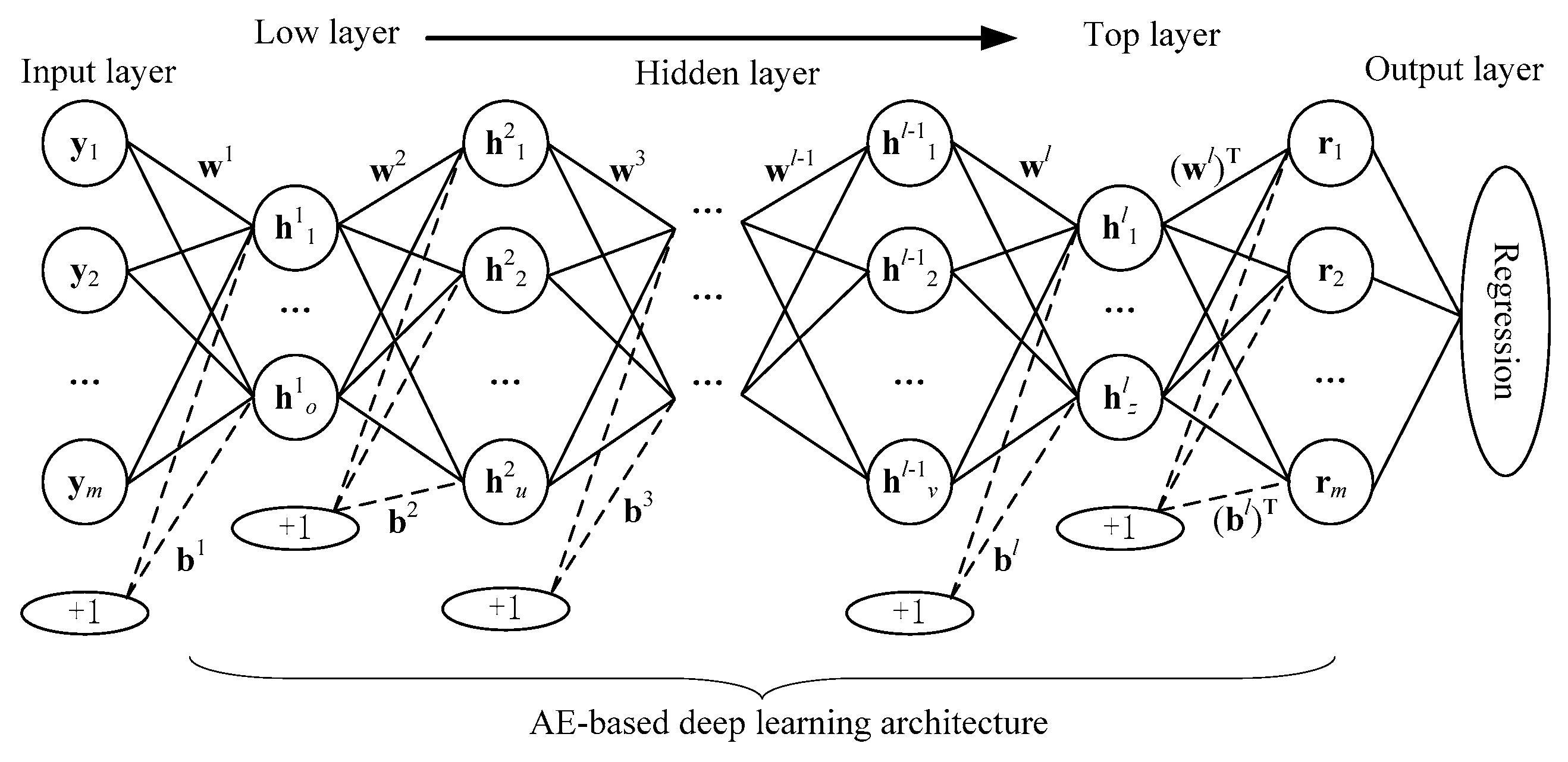
Figure 1. Structures of the autoencoder (AE)-based deep regression network (DRN) model. wl and bl represent the connection weight matrix and bias values between neighboring layers ((l-1)-th and l-th layers), respectively.
Applsci 10 02522 g001
Figure 2. Flow chart of the proposed manifold learning-based deep regression network (MDRN) approach for multi-parameter manufacturing quality prediction.
Applsci 10 02522 g002
Figure 3. Manufacturing quality of different batches: (a) Case 1 and (b) Case 2.
Applsci 10 02522 g003
Figure 4. Testing results of different MDRN models with different K: (a) K = 8, (b) K = 10, (c) K = 12, and (d) K = 14.
Applsci 10 02522 g004
Figure 5. Prediction results of the MDRN model with 3-30-30-1 of Case 1: (a) plots the comparison with the measured and the predicted values, and (b) shows the residual error distribution.
Applsci 10 02522 g005
Figure 6. Prediction results of the MDRN model with 3-30-30-1 of Case 2: (a) plots the comparison with the measured and the predicted values, and (b) shows the residual error distribution.
Applsci 10 02522 g006
Figure 7. Prediction results of Case 1 using different models. (a) AE-based DRN with 19-25-25-1, (b) least squares support vector regression (LSSVR), and (c) BPNN with 19-10-1.
Applsci 10 02522 g007
Figure 8. Prediction results of Case 2 using different models. (a) AE-based DRN with 19-40-40-1, (b) LSSVR, and (c) back propagation neural network (BPNN) with 19-12-1.
Applsci 10 02522 g008aApplsci 10 02522 g008b
Table 1. Statistical information of the multi-parameter in different processes.
Multi-ParameterProcessRange
Parameter 1 (x1)Pro-processingAdjustable0, 1, 2, 3, 4, 5
Parameter 2 (x2)0, 1
Parameter 3 (x3)No-adjustable[7, 30.304]
Parameter 4 (x4)[7, 30.304]
Parameter 5 (x5)0, 1
Parameter 6 (x6)ManufacturingAdjustable0, 1
Parameter 7 (x7)342, 343
Parameter 8 (x8)0.065, 0.075, 0.28
Parameter 9 (x9)0.4, 1
Parameter 10 (x10)1, 1.05, 1.3
Parameter 11 (x11)0, 0.34, 0.35
Parameter 12 (x12)0, 1, 2
Parameter 13 (x13)0, 1, 3, 4
Parameter 14 (x14)0, 1
Parameter 15 (x15)No-adjustable4, 6
Parameter 16 (x16)[1, 110]
Parameter 17 (x17)0, 1
Parameter 18 (x18)0, 1, 2, 3, 4, 5
Parameter 19 (x19)3, 3.1, 3.6
Table 2. Experimental designing of each approach.
ModelExperimental Design
K-Isomap for dimension reductionK = [8, 10, 12, 14]
DRN for manufacturing quality predictionStructure parameters: l = [1, 2, 3], hidden nodes in each hidden layer = [10, 15, 20, 25, 30, 40, 50].
Computing parameters: dropout 0.5, learning rate 1, batch-size 10, and iteration 200.
Table 3. Quantitative results in training and testing process using the proposed model.
CasePerformance (Training)
MAPE (%)RMSETS1 (%)TS5 (%)TS10 (%)
11.5750.02032.6100100
21.4140.02044.4100100
CasePerformance (Testing)
MAPE (%)RMSETS1 (%)TS5 (%)TS10 (%)
11.9430.0222795100
21.8610.02335.595.599.5
Table 4. Comparison of the prediction performances using different models.
CaseModelPerformance
MAPE (%)RMSETS1 (%)TS5 (%)TS10 (%)
1Proposed model1.9430.0222795100
AE-based DRN2.3880.033259196
LSSVR2.5430.034249196
BPNN3.2100.044268393
2Proposed model1.8610.02335.595.599.5
AE-based DRN2.2010.03134.59397
LSSVR2.2910.032329397
BPNN2.7570.03830.585.595