Reciprocating Compressor Multi-Fault Classification Using Symbolic Dynamics and Complex Correlation Measure

Abstract

Prognostics and Health Management technologies are useful for early fault detection and optimization of reliability in mechanical systems. Reciprocating compressors units are commonly used in industry for gas pressurization and transportation, and the valves in compressors are considered vulnerable parts susceptible to failure. Then, early detection of faults is important for avoiding catastrophic accidents. A feasible approach for fault detection consists in measuring the vibration signal for extracting useful features enabling fault detection and classification. In this research, a test-bed composed by two-stage reciprocating compressor was used for simulating a set of 13 different conditions of combined faults in valves and roller bearings. Three accelerometers were used for collecting the vibration signals for extracting three different types of features. These features were analyzed furthermore by using two random forest models to classifying the different faults. The first set of features was obtained by applying the symbolic dynamics algorithm, which provides the histogram of a set of symbols. This set of symbols was obtained by subdividing a 2D Poincaré plot into angular regions and counting the intersection of the phase trajectories on each of regions. The second type of features corresponds to the complex correlation measure which is calculated as the addition of the areas of triangles belonging to a Poincaré plot. Additionally, a small set of classical statistical features was also used for comparing their classification abilities to the new set of proposed features. The three sets of features enable highly accurate classification of the set of faults when used with random forest classification models. Notably, the ensemble subspace k-Nearest Neighbors algorithm provides classification accuracies higher than 99%.

1. Introduction

Reciprocating compressors generally work continuously at full load and many times without a backup, then maintenance management must guarantee maximum efficiency, avoid unscheduled stops, and decrease maintenance times. All this is a challenge because the compressors are elements that work in extreme working conditions such as high temperatures, variable pressures, and alternative movements. As consequence, its critical elements such as valves and roller bearings are more likely to failure [1,2,3,4]. In this context, the application of Prognostics and Health Management (PHM) technologies is important to develop intelligent fault diagnosis systems to guarantee high reliability in the operation and avoid catastrophic damages [5]. Several types of signals are useful for fault diagnosis in reciprocating compressors, such as vibration, acoustic emission, electric current, pressure and temperature [6]. Vibration signals have been studied, for both signal analysis to detect faults [4,7] and for fault classification [8]. Compressor are reciprocating machines that works with different mechanical multi-component coupling elements, and the vibration signals have non-linear and non-stationary characteristics [9].

Several research works applying PHM technologies in reciprocating compressors have been reported. A research concerning the condition monitoring of the valves by using analytical and data-driven technologies is reported in [10]. The research analyzes different valve failure modes, and also investigates the type of sensors useful for detecting such faults. The fault diagnosis of reciprocating compressor valves using information entropy and Support Vector Machines (SVM) is reported in [11]. The extraction of information entropy features was performed on vibration signals for classifying three types of valve conditions: normal, slightly damaged and severe damaged. An approach for detecting cracked or broken valves under varying load conditions is reported in [4]. The approach is based on time-frequency analysis of the vibration signal. The fault detection is based on the comparison between the spectrogram of the vibration signal and a reference spectrogram representing a healthy valve. The method provides high classification accuracy considering different load conditions. A method for fault detection in reciprocating compressor valves using basic pursuit, wave matching and SVM is reported in [12]. The features used for classification are extracted by wave matching of the vibration signal, regarding a parameterized waveform that is optimized by using a differential evolution algorithm. This approach is used for classifying three valve conditions including the normal condition, spring deterioration and valve plate deformation. The algorithm attains classification accuracies up to 100%.

Research concerning the modeling of reciprocating compressors uses phase space trajectories, Poincaré maps, and large Lyapunov exponents for identifying the chaotic behavior of a reciprocating compressor system with a subsidence rub-impact fault [13,14]. Non-linear and chaotic dynamical systems can be analyzed by using tools like the phase space diagram and the Poincaré plot [15]. The phase space diagram is used for visualizing the behavior of dynamical systems by representing the trajectories such as a 3D trajectory for a chaotic system [16]. The Poincaré map is obtained from the phase space diagram by sampling points in the phase space. For instance, for the case of a 3D phase space, the Poincaré section is obtained from the interception of the phase space trajectories with a plane. The Poincaré map (also known as Poincaré section) has been used for visualizing non-linear, chaotic behavior of faults in gears and bearing elements [17]. Estimation of features extracted from Poincaré maps aiming at fault characterization has been reported in [18]. In that research, authors proposed a damage index that is calculated based on the length of the phase space represented by the Poincaré map. Additionally, a nonlinear dynamical system can be analyzed by studying their dynamics using a topological partition of the phase space [19] that is known as the Symbolic Dynamics (SD). When dealing with signal processing applications, SD enables the transformation of the signals into sequences of symbols that enhance the non-linear features useful for detection or classification.

Although several research studies for classifying faults in reciprocating compressors have been reported, most of the research has been focused on studying a small set of valves faults. This has motivated to set up a test-bed platform that enables investigation of a more extensive set of faults in valves as well as combined faults of valves and roller bearings. In the previous research [20], a deep learning approach based on long short-term memory (LSTM) models has been used for classifying 17 different faulty conditions in valves of a two-stage reciprocating compressor. The multi-fault dataset considers combinations of faults in the intake and discharge valves of the first and second stages. Each of the valves is affected by one of the following simulated valve faults: seat wear, plate corrosion, plate fracture and broken spring. The proposed approach attained a classification accuracy up to 93%.

This paper proposes the use of Symbolic Dynamics (SD) and Complex Correlation Measure (CCM) as novel features for fault diagnosis in rotating machinery, as an alternative regarding complex computational architectures such as deep learning approaches. We used the same test-bed platform in [20] to investigate the classification of combined faults of valves and roller bearing by using vibration signals, also called “multi-fault scenario”. The dataset of combined faults of valves and roller bearings considers the same set of four basic fault conditions for the discharge valve of the second stage of the compressor, in combination with three common faults of the roller bearings. Additionally, we also test the proposed features with the valve faults dataset in [20] and perform the comparison to that previous research, in order to highlight the proper classification accuracy regarding the use of deep learning architectures. The original contributions of this paper are the following:

• Novel application in PHM of the Complex Correlation Measure (CCM) derived from the Poincaré plot of the vibration signal for extracting useful features for accurate classification of multi-fault in valves and roller bearings.
• Novel application of Symbolic Dynamics (SD) for classification of multi-fault of valves and roller bearings.
• Accurate classification of 13 different combined fault conditions (multi-fault scenario) of valves and roller bearing.
• Accurate classification of 17 fault conditions of valves in a reciprocating compressor.
• Comparison of three different set of features extracted from vibration signal for classifying the set of multi-fault previously mentioned.
• Comparison of two high performance Random Forest (RF) models applied to the problem of multi-fault classification of valves and roller bearings in a reciprocating compressor.

2. Poincaré Plot and Their Features

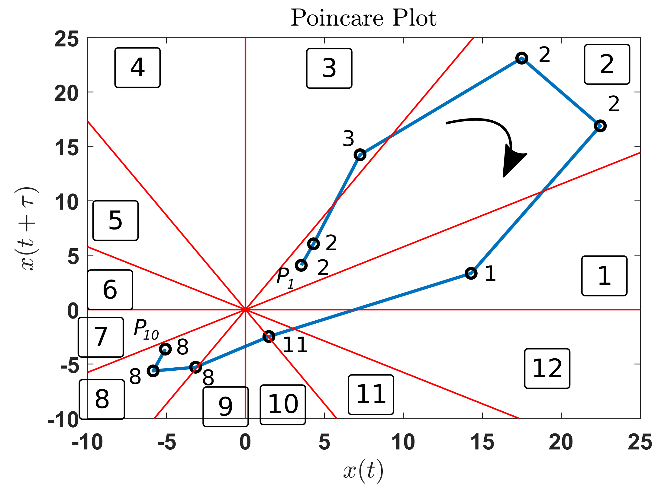
2.1. Poincaré Plot

The Poincaré plot is related to the Poincaré map that is used for studying non-linear dynamics of chaotic systems [21]. A physical system can be represented as a set of first-order differential equations:

$$\dot{x}=\frac{dx}{dt}=f\left(x\right),x\in {\mathbb{R}}^n,$$

(1)

where f is a smooth vector field. The solution for this set of equations is denoted $\varphi (x,t)$, that can satisfy $\varphi (x,0)=x$. The expression $o\left(x\right)=\{\varphi (x,t)/x\in {\mathbb{R}}^n\}$ is known as an orbit or trajectory in the phase space. The Poincaré map is obtained by considering successive intersections of a trajectory with a lower-dimensional surface denoted $\Sigma$ of the phase space ${\mathbb{R}}^n$ as shown in Figure 1.

In general, the Poincaré map is well defined when the system has periodic solutions. In this case there exists a positive number T representing the orbit period. Similarly, the system has an initial solution denoted $x^{\left(0\right)}$. The solution satisfies $\varphi (x^{\left(0\right)},T+t)=\varphi (x^{\left(0\right)},t)$ for all $t\in \mathbb{R}$. Particularly, $\varphi (x^{\left(0\right)},T)=\varphi (x^{\left(0\right)},t)=x^{\left(0\right)}$ then the point $x^{\left(0\right)}$ returns to himself after flowing during the time T. The Poincaré map reduces the dimension of the problem by one because the system can be studied by considering only the points included in $\Sigma$. Unfortunately, except for trivial cases, the Poincaré map cannot be expressed explicitly [16]. In general, the Poincaré map construction requires solving the set of differential equations and detecting the points where the orbits intercept the surface $\Sigma$. The Poincaré map has the property of reflecting characteristic features of the flow $\varphi (x,t)$. For instance, stable or regular trajectories result in simple curves when they are represented in the map. In contrast, unstable or chaotic trajectories result in sequences of random points in the Poincaré map.

In practical engineering applications, we deal with complex problems where accurate knowledge about the physical relations of different parts of the system is not available. There is not any mathematical model for such a system, and sometimes we only have a measurement of a given variable as a function of time, such as a vibration signal denoted $x\left(t\right)$. In these cases, the Poincaré map cannot be calculated. Then, approximate solutions are provided such as plotting the estimated first derivative of the time series $dx\left(t\right)/dt$ with respect to $x\left(t\right)$ [22], or plotting each value of the time series $x\left(t\right)$ with respect to their delayed version $x(t-d)$, or equivalently $x(t+d)$ versus $x\left(t\right)$ [21]. This type of plot is known as delay-coordinate reconstruction, delay plot or, in the domain of application of biomedical engineering, it is known as the Poincaré plot [23]. An illustration of this concept is shown in Figure 2, where the 3D representation of the Lorenz attractor is depicted in terms of the phase-space trajectories [24]. The Lorenz model was developed for studying atmospheric convection. However, their application has been extended to other domains such as electric circuits and brushless DC motors. The Lorenz model is composed by a set of three ordinary differential equations:

$$\frac{dx}{dt}=\sigma (y-x)$$

(2)

$$\frac{dy}{dt}=x(\rho -z)-y$$

(3)

$$\frac{dz}{dt}=xy-\beta z$$

(4)

where the parameters are the Rayleigh number $\rho$ or, the Prandtl number $\sigma$, and an additional parameter $\beta$.

Typical values are $\rho =28$, $\sigma =10$ and $\beta =8/3$. Given an initial point $(x_0,y_0,z_0)$, the system of equations is solved and the evolution of each of the variables is represented as a 3D phase space. Such phase space is intersected with a surface $\Sigma$ representing a plane. The intersection points in this 2D surface represent the Poincaré map, as shown in Figure 3.

2.2. Symbolic Dynamics

When dealing with a non-linear dynamical system such as the Lorenz model in Equations (2)–(4) with a phase space represented in Figure 2, the n-dimensional phase space can be partitioned into a finite set of contiguous cells, and each of the cells is assigned to a symbol [25]. A trajectory in the phase space generates a sequence of symbols describing the dynamics of the system.

In this research, rather than partitioning the n-dimensional space, we propose the partition of the 2D surface $\Sigma$ representing the interception of the current phase space with a plane. A 2D representation of the Lorenz model is shown in Figure 4. The dynamics of this model is represented in terms of their components $x\left(t\right)$, $y\left(t\right)$ and $z\left(t\right)$ and their representation in $\Sigma$ can be approximated by using the Poincaré plot as shown in Figure 4. Such a plot is constructed by using only the component $x\left(t\right)$; however, it can recover important features of the underlying dynamical system. In practical applications, such as fault detection in rotating machinery using vibration signals, the current underlying dynamical system is generally unknown and in the best of cases only approximate models are provided. The only known information is the time series representing the vibration signal, in consequence, we are constrained to attain a useful system representation using this information. When dealing with a dynamical system as previously described, the surface $\Sigma$ of the phase space can be partitioned into r disjoint subsets denoted $p=\{P_1,P_2,P_3,\dots ,P_r\}$. Each subset is represented by a symbol $r\in \{1,2,3,\dots ,r\}=S$. An orbit in the phase space is represented by a sequence of visited symbols $\mathbf{s}=\{s_1,s_2,s_3,\dots ,\}$ [26]. The surface can be arbitrarily subdivided into several cells, and the points of the Poincaré plot located in each cell can be represented by the same symbol. Alternatives of feasible partitions are Voronoid tessellations [27], or fractal based tessellations [28]. The sequence of generated symbols can be used for constructing state machines using sliding block codes [29] where a window of length $N_w$ is shifted to the right one symbol at a time for constructing a $N_w$-Markov machine useful for anomaly detection [25]. In a previous research concerning faults classification in gearboxes, the Poincaré plot has been subdivided in a set of angular regions and each region has been represented by a symbol. An illustration of this concept is presented in Figure 5. A fragment of a trajectory in the Poincaré plot is shown and each point in the trajectory is assigned to a symbol according to the location of each point. Each angular region corresponds to one symbol and the partition of the phase space includes 12 symbols: $S=\{1,2,3,4,5,6,7,8,9,10,11,12\}$. In this example, the trajectory is represented by the set of symbols $\mathbf{s}=\{2,2,3,2,2,1,11,8,8,8\}$. The count of points corresponding to each symbol provides a set of features that can enable fault classification. This is illustrated in Figure 6 where the Poincaré plot constructed with component $x\left(t\right)$ for the Lorenz model is shown along the angular partition of $\Sigma$. The histogram of symbols calculated for this partition is shown in Figure 6b.

2.3. Complex Correlation Measure

The Complex Correlation Measure (CCM) is a feature that quantifies the temporal variation of the signal based on the Poincaré plot. This feature was proposed for the diagnosis of cardiac diseases based on the heart rate interval signals [30]. This feature is calculated from a lagged Poincaré plot by using a sliding window of three consecutive samples represented in the Poincaré plot. For a 2D Poincaré plot, the sliding window includes three consecutive points that forms a triangle, and the area of this triangle is calculated and added by considering all signal samples. This concept is illustrated in Figure 7 for a Poincaré plot constructed for a lag $\tau$. Let $X=\{x_1,x_2,x_3,\dots ,x_N\}$ be the vibration sampled signal, and consider the i window including the points denoted $a(x_i,y_i)$, $b(x_{i+1},y_{i+1})$ and $c(x_{i+2},y_{i+2})$, where $y_i=x_{i+\tau }$. The area of the triangle spanned by points (a,b,c) is calculated as:

$$A\left(i\right)=\frac{1}{2}\left|\begin{array}{ccc}{x}_i& y_i& 1\\ x_{i+1}& y_{i+1}& 1\\ x_{i+2}& y_{i+2}& 1\end{array}\right|$$

(5)

The area is 0 when points a, b and c are on a straight line. The area is positive when points have a counter clock-wise orientation. In contrast the area is negative for clock-wise orientation. The CCM considering a Poincaré plot with M points is obtained by adding the area within the sliding window as:

$$CCM\left(\tau \right)=\frac{1}{C_m}\sum _i^{M-2}A\left(i\right),$$

(6)

where $\tau$ represents the lag used for constructing the Poincaré plot, $C_m$ is a normalizing constant set as $C_m=1/(M-2)$. The number of points of the Poincaré plot is $M=N-\tau$ with N representing the number of samples of the vibration signal.

3. Random Forest

Random Forest (RF) algorithm is a methodology based on ensemble methods that use a set of weak learners such as tree-type classifiers which are combined to provide a high-quality classification or regression models [31]. When the ensemble method uses the tree-type classifiers as weak learners, the RF algorithm works by growing M different randomized trees using bootstraps resampling [32,33]. Each base learner (tree) is grown by using the CART (Classification And Regression Tree) methodology. Starting from the root node, the data is split into two children and each children is, in turn, split into two grand-children. At each node, rather than choosing the best split among all features, a subset of features is randomly sampled and the best split is selected among those features using the Gini impurity index [34]. The process stops when there are not more splits due to the lack of data. Each of the trees of the RF is grown by using a training set that is extracted with replacement from the original training set. The training set used for growing a particular tree is subdivided into two portions: the In Bag data corresponds to $2/3$ of the data used for training the tree, and the Out of the Bag (OOB) data corresponds to $1/3$ of the data which is also extracted at random from the training data set. The OOB is used for validation of the tree. A voting system is implemented for providing the final classification based on the results provided by each individual tree [35]. In this research two types of RF algorithms are used: ensemble bagged trees [31] and ensemble subspace k-Nearest Neighbors (k-NN) where the weak learner is the k-NN algorithm trained with random samples of features [36,37].

3.1. Ensemble Bagged Trees

This machine learning model consists of tree predictors that are aggregated to attain a more accurate predictor. The bagging approach was proposed by Breiman [38] for constructing classifiers using bootstraps re-sampling [33].

A learning dataset is denoted $\mathbf{X}=\{({\mathbf{x}}_n,y_n),n=1,2,3,\dots ,N\}$ where ${\mathbf{x}}_n$ includes the features and $y_n$ are the labels. Bagging techniques rely on the application of bootstrapping that is performed by using random sampling with replacement. Then, the learning dataset can be processed for obtaining bootstraps replicates that are denoted ${\mathbf{X}}^b=\{({\mathbf{x}}_n^b,y_n^b),n=1,2,3,\dots ,N\}$. The original learning dataset can be used for constructing a learning classifier denoted $\mathbf{C}(\mathbf{x},\mathbf{X})$ that performs the prediction of label y based on features $\mathbf{x}$. When each bootstrapping replicate is used for training a classifier, the result is a set of classifiers denoted $\{{\mathbf{C}}^b(\mathbf{x},{\mathbf{X}}^{\mathbf{b}}),b=1,2,3,\dots ,B\}$. More accurate classifier ${\mathbf{C}}_A^b\left(\mathbf{x}\right)$ can be obtained by aggregating the set of classifiers constructed with the bootstrapping replicates. Several alternatives for aggregation can be considered such as the averaging:

$${\mathbf{C}}_A^b\left(\mathbf{x}\right)=\sum _{b=1}^B{\mathbf{C}}^b(\mathbf{x},{\mathbf{X}}^{\mathbf{b}})$$

(7)

This averaging rule is useful for aggregating linear classifiers by averaging their coefficients in order to obtain a linear classifier. An additional approach for aggregating is a voting system. When the classifier is used for predicting a class $j\in \{1,2,3,...J\}$ by using the set of trained classifiers, the set $N_j=\#\{k;{\mathbf{C}}^k(\mathbf{x},{\mathbf{X}}^{\mathbf{k}})=j\}$ including the results can be defined. In this case the aggregation is performed as:

$${\mathbf{C}}_A^b\left(\mathbf{x}\right)=argma{x}_j{N}_j$$

(8)

representing the class for which $N_j$ has the maximal cardinality. Several classifiers can be used, however, tree based classifiers are commonly used. In the original research, Breiman showed that misclassification can be reduced with rates ranging from 6% to 77% by using bagging techniques.

3.2. Ensemble Subspace k-Nearest Neighbors

In the Ensemble subspace k-NN, the basic classifier is the k-Nearest Neighbors and a set of classifiers are trained using different modified bootstraping replications of the training data. This approach was proposed by Tin Kam Ho [36]. Each training object denoted ${\mathbf{x}}_n$ in the learning dataset $\mathbf{X}=\{({\mathbf{x}}_n,y_n),n=1,2,3,\dots ,N\}$ is a r-dimensional vector ${\mathbf{x}}_n=[x_{n,1},x_{n,2},x_{n,2},\dots ,x_{n,r}]$ including r features. According to the random subspace method $p<r$ features are randomly selected from the r-dimensional training dataset $\mathbf{X}$. The modified training dataset is denoted ${\tilde{\mathbf{X}}}^b=\{({\tilde{\mathbf{x}}}_n^b,{\tilde{y}}_n^b),n=1,2,3,\dots ,N\}$ where each training object is a p-dimensional array ${\tilde{\mathbf{x}}}_n^b=[x_{n,1},x_{n,2},x_{n,2},\dots ,x_{n,p}],(n=1,2,3,\dots ,N)$. The modified training dataset is constructed using the same set of p features for each ${\tilde{\mathbf{x}}}_n^b$. A set of B classifiers is trained by using ${\tilde{\mathbf{X}}}^b$ and then they are aggregated through a simple majority voting system.

4. Experimental Test-Bed

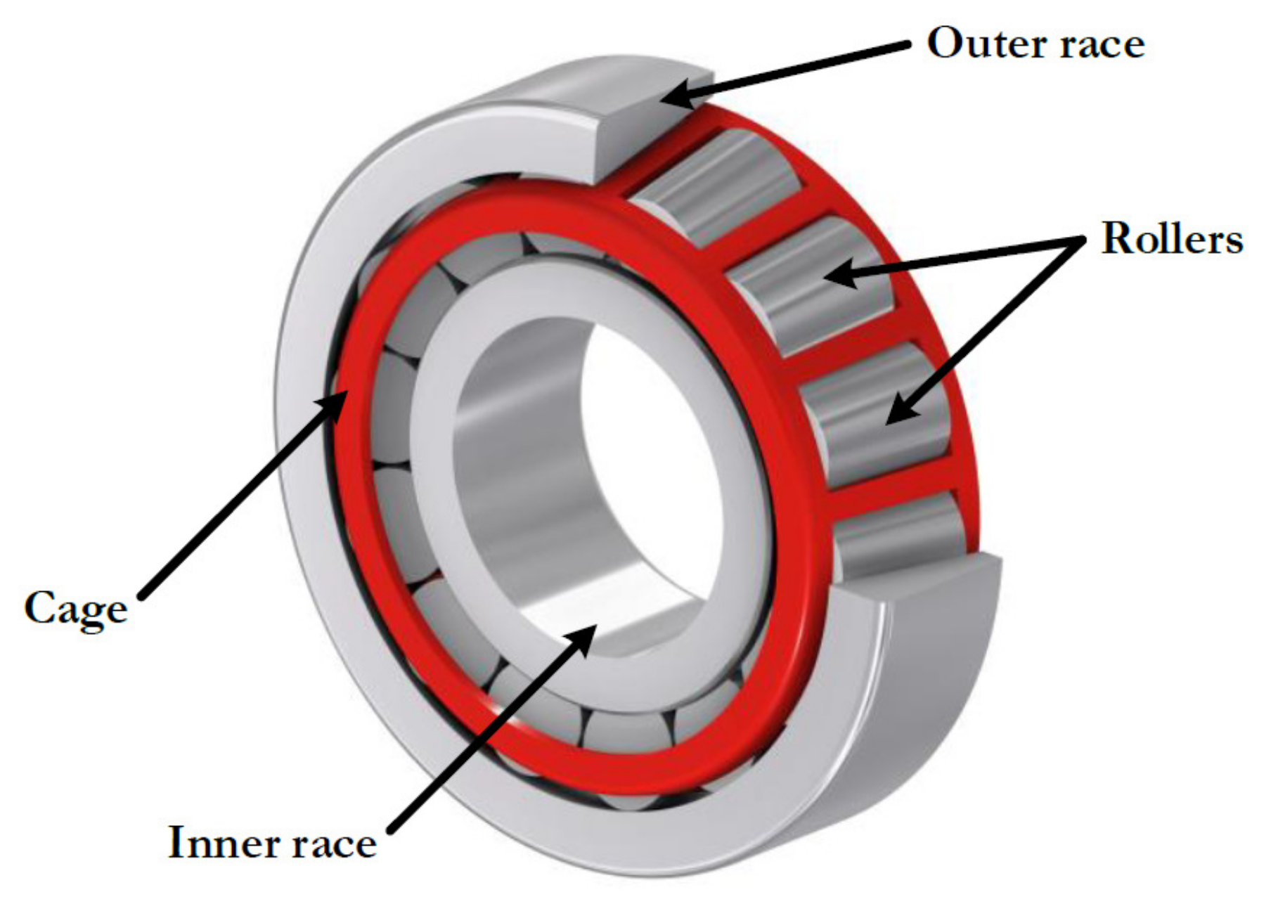
4.1. Reciprocating Compressor

A reciprocating compressor model EGB-250 driven by a 5.5 hp induction motor was used in the experiments. Mechanical rotatory motion at 3470 rpm is transmitted to the compression chamber using two V-belts. The compressor has two stages, both with two valves: one for inlet and one for discharge. The second stage enables the transfer of the gas to the tank. The compressor used in this research is shown in Figure 8. The main elements studied in this research are the roller bearings and the valves. Tapered roller bearings are used due to their ability to withstand high combined loads. They are mounted on ‘X’ (face to face) one on each side of the crankshaft. An schematic view of the tapered roller bearing showing each of their parts is presented in Figure 9. The type of valve used is presented in Figure 10a and the assembly form in Figure 10b. This valve works as an intake valve or as a discharge valve. Its operation mode depends only on the orientation in which it is assembled.

In this research, fault combinations in bearings and valves were considered. Faults were introduced in the roller bearing B1 which is located closer to the fan pulley and in the discharge valve located in the second stage. Three type of faults are included for the roller bearing: (a) inner race crack, (b) roller element crack and (c) outer race crack. The cracks are created through the Electrical Discharge Machining (EDM) technique. The inner and outer race cracks are aligned with the rotation axis and covers all the raceway. They have a width of 2.0 mm and a depth of 1.0 mm. The roller element crack is also aligned with the rotation axis. It has a width of 1.0 mm and a depth of 0.5 mm.

Concerning the valves, four types of faults were included: (1) valve seat wear, (2) corrosion of the valve plate, (3) fracture of the valve plate and (4) broken spring. The different conditions of the valves are shown in Figure 11. The valve seat wear is attained by machining on the face of the valve seat and reducing its depth 1.44 mm. The corrosion of the valve plate is simulated by performing a through hole with a diameter of 2.5 mm. The fracture of the valve plate is performed by cutting the plate, the diameter of the thread is 1.6 mm. The break of the spring is obtained by cutting the spring with a thread of 1.6 mm of diameter.

In total, 13 different multi-fault classes were considered. P1 denotes the healthy class and classes P2-P13 correspond to 12 combinations of one fault type in the roller bearings with each one of the four possible faults in the valve. The fault combinations are described on

Table 1. Multi-faults in valve and roller bearings.

Label	Valve, 2S–DV	Bearings, B1
P1	Healthy	Healthy
P2	Valve seat wear	Inner race crack
P3	Corrosion of valve plate	Inner race crack
P4	Fracture of valve plate	Inner race crack
P5	Broken Spring	Inner race crack
P6	Valve seat wear	Roller element crack
P7	Corrosion of valve plate	Roller element crack
P8	Fracture of valve plate	Roller element crack
P9	Broken Spring	Roller element crack
P10	Valve seat wear	Outer race crack
P11	Corrosion of valve plate	Outer race crack
P12	Fracture of valve plate	Outer race crack
P13	Broken Spring	Outer race crack

. The internal and external parts of the reciprocating compressor used for dataset acquisition are shown in Figure 12.

4.2. Dataset Vibration Signal Acquisition

Three accelerometers denoted A1, A2 and A3 (model PCB 603C01) were vertically placed on the compressor case. A1 is located close of the discharge valve, A2 is located close of the intake valve of the second stage. A3 is located close to the B1 roller bearing. A plot showing the location of each accelerometer is presented in Figure 13. Although other sensors are located in the test-bed for recording signals such as current, sound, acoustic emission and pressure, they are not considered in this paper.

The analog signals were transferred using a coaxial-cable to a National Instruments model NI-9234 compact data acquisition card (cDAQ) connected to the NI-9188 chassis to stream the digital signals to a laptop computer through a 100 Mbps Ethernet Link. The acquisition process is controlled using a LabView software running on a laptop for performing the A/D conversion and storing the data in a hard-disk for off-line processing. The measurements were taken under a 57.7 Hz constant motor rotation frequency, resulting in a 12.8 Hz crankshaft rotation frequency. There are two crankshaft cycles per compression cycle, in consequence, the total compression cycle takes approximately 0.156 s. The tank pressure was kept constant at 3 bar. A set of 15 vibration signals for each sensor and for each machinery condition was collected. A total of $15\times 13=195$ signals of 10 s each were digitized at sampling frequency of 50 kHz.

5. Feature Extraction

Three types of features were considered in this research. The first type of features were extracted from the Symbolic Dynamics (SD). The second type of features is the Complex Correlation Measure (CCM) extracted from the Poincaré plot. Finally, a set of classical statistical features are considered for comparison based on their classification accuracy.

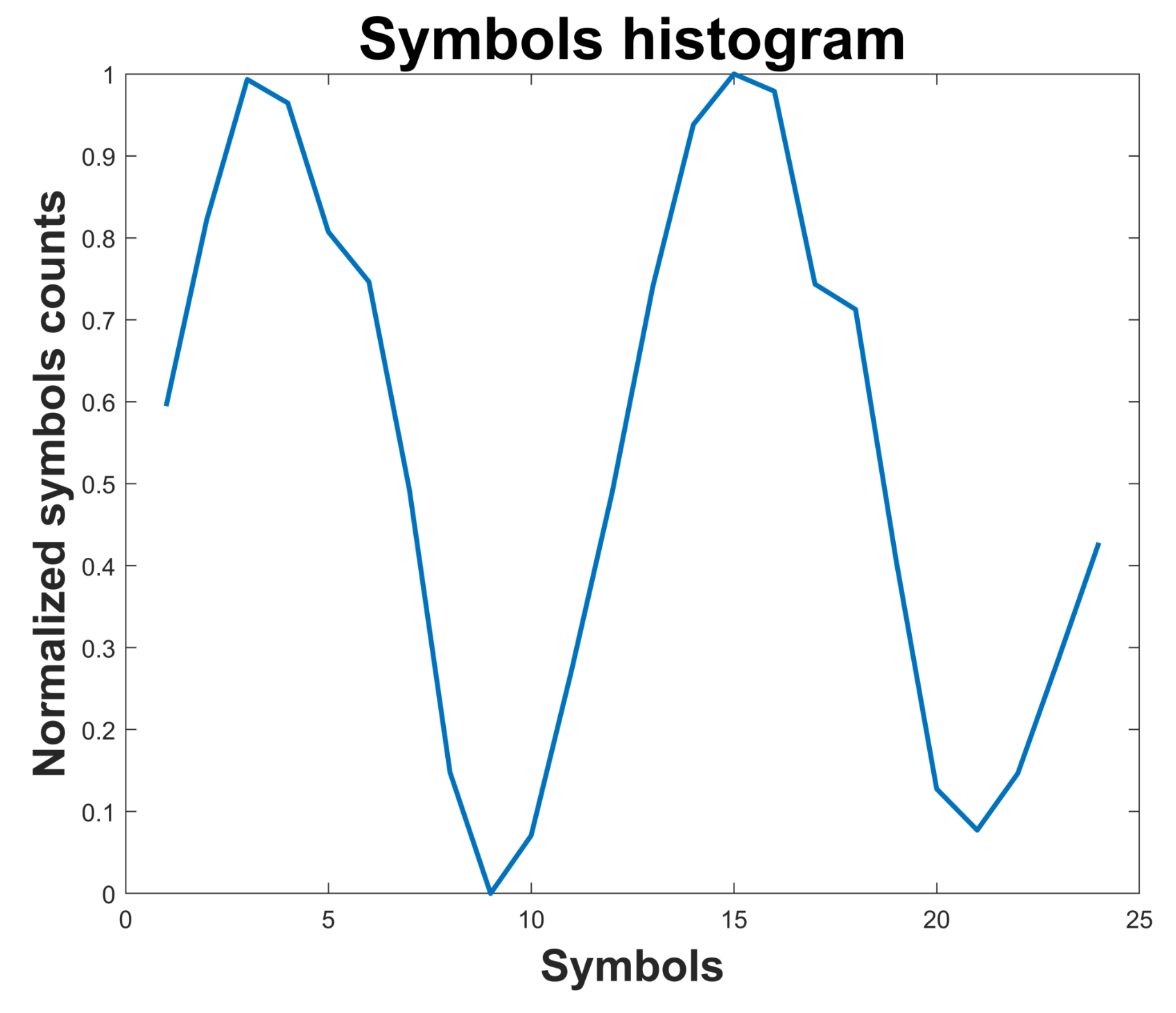
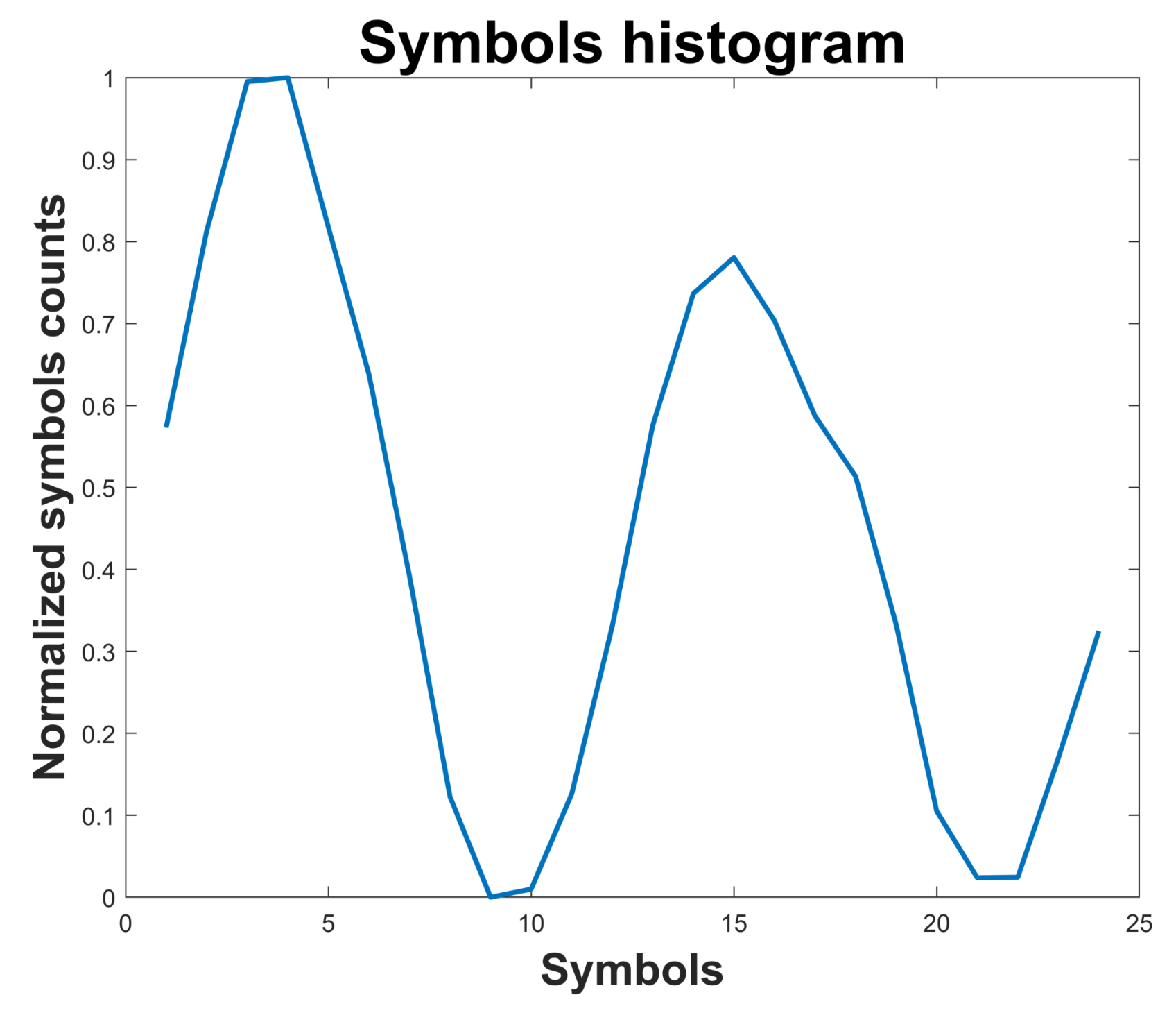
5.1. Symbolic Dynamics

This paper uses the SD feature extraction algorithm in [26], which is summarized in the following steps: (1) The Poincaré plot is traced using a lag of 15, (2) The phase-space represented by the Poincaré plot is subdivided into several angular regions as shown in Figure 14, (3) Each region is assigned to a symbol represented by an integer number, 24 angular regions are considered in this application, (4) The symbolic representation of the vibration signal is processed for obtaining the histogram. This is simply attained by counting the number of points in each angular region.

An example of the histogram obtained for a vibration signal of the reciprocating compressor considering the healthy state P1 is shown in Figure 15. Similarly, the histogram for the faulty state P5 is shown in Figure 16. The array including 24 elements of the histogram is considered as Symbolic Dynamic (SD) feature useful for fault classification. In the faulty case corresponding to P5, the second peak in the histogram has lower amplitude as compared to the healthy case.

5.2. Complex Correlation Measure

Calculation of the Complex Correlation Measure (CCM) does not require the explicit plotting of the Poincaré plot. The calculation is performed over the original time series of the vibration signal denoted $X=\{x_1,x_2,x_3,\dots ,x_N\}$ as well as their delayed version $X_{\tau }$. The i window includes the points denoted $a(x_i,y_i)$, $b(x_{i+1},y_{i+1})$ and $c(x_{i+2},y_{i+2})$ where $y_i=x_{i+\tau }$. With this information, Equations (5) and (6) are evaluated. The CCM of the vibration signals was calculated for $\tau$ varying between 1 and 50. An example of this feature set is shown in Figure 17 for a signal extracted from the healthy class $P1$ and for the faulty class $P2$. In general the amplitude of the CCM feature is higher for the faulty class when compared to the normal class.

5.3. Statistical Features

A set of classical statistical features was considered for comparing to the performance of the proposed CCM and SD features. The set of statistical features has been studied in [39] for detection of multi-fault in roller bearings and gearboxes. The features are the mean value, root mean square value, standard deviation, kurtosis, maximum value, crest factor, rectified mean value, shape factor, impulse factor, variance, minimum value and skewness. This set corresponds to a 12-dimensional array.

6. Multi-Fault Classification

Figure 18 depicts the methodology for multi-fault classification. In the first stage, vibration signals of 13 conditions were acquired, and each condition is repeated 15 times, all the signals of 10 s length, i.e., 195 signals per class. In the pre-processing stage, each signal is subdivided into five fragments of 2 s, obtaining 975 samples for the 13 conditions. In the third stage of feature extraction, for each of fragments three different sets of features are extracted: (a) the statistical features set is composed of 12 features, (b) the SD is represented by a set of 24 features, and (c) the CCM features are composed of 50 features. For the classification stage, each feature dataset is split into a test set (16%) and a training set (84%). Two types of classifiers are trained and 10-fold cross-validated: The Ensemble Bagged Tree (EBT) [31] and the Ensemble Subspace k-NN (ESK) [37]. The classification accuracy of each trained classifier is evaluated over the test dataset. This procedure is repeated for each of the vibration signals collected from the accelerometers A1, A2 and A3, and the results are compared.

Parameters Selection

Parameters for feature calculation are set in a heuristic manner. The first parameter corresponds to $\tau$ that is used for calculation of CCM features. The CCM features are calculated by varying $\tau$ between 1 and 60 for the vibration signal A1. The fault classification is performed by using the EBT algorithm, and the accuracy is plotted as a function of $\tau$. The results are shown in Figure 19. The accuracy increases as $\tau$ increases, and it settles at $\tau =45$. In consequence, we can set $\tau =50$ for the rest of experiments. Similarly, calculation of SD features requires previous construction of the lagged Poincaré plot according to the lag $\tau$. In this case, $\tau$ is varied between 5 and 60. For each lag value, the SD features are calculated from signal A1, and the fault classification model uses the EBT algorithm. The accuracy is plotted with respect to the lag value, and the lag value $\tau =15$ corresponds to the maximal accuracy obtained in classification. The plot is shown in Figure 20.

The parameters for the classification models are the maximum number of splits and the number of learning cycles for the EBT algorithm. In this case, the maximum number of splits is set as $n-1$ where n is the number of samples in the training set. The number of learning cycles is 36. The algorithm ESK considers 30 learning cycles, and the number of predictors to sample is set as half the number of predictors of the features set.

7. Results

Results concerning the multi-fault classification are shown on

Table 2. Percent accuracy for each of features types and models calculated for each vibration signal.

Features	Model	A1	A2	A3
Statistical	EBT	100	100	100
	ESK	100	100	100
SD	EBT	100	100	100
	ESK	100	100	100
CCM	EBT	99.4	96.8	94.2
	ESK	100	100	99.4

. The SD and CCM features are considered as well as the statistical features that are presented for comparison. Both RF classification algorithms are tested for each of the vibrations signals. The statistical set of features and the SD set of features enable perfect classification of multi-fault for this dataset including 13 different fault conditions. The CCM set of features provides slightly lower classification accuracy. However, the ESK algorithm attains averaged classification accuracies higher than 99% for the three vibrations signals collected from the accelerometers A1, A2, A3. An example of the confusion matrix is shown in Figure 21. This confusion matrix is for the EBT algorithm when the multi-fault classification is performed using the set of signals collected from the accelerometer A3. The average accuracy obtained in this case is the lowest of all developed experiments. A detailed quantification of results for this particular case are shown on

Table 3. Results for the EBT model using features extracted from signals recorded with the accelerometer A3.

Fault Condition	Sensitivity	Specificity	F1-Score
P1	0.92	1.00	0.96
P2	1.00	1.00	1.00
P3	1.00	1.00	1.00
P4	1.00	0.99	0.96
P5	1.00	0.99	0.96
P6	0.92	1.00	0.96
P7	0.92	0.99	0.92
P8	0.85	0.99	0.88
P9	1.00	0.99	0.96
P10	1.00	1.00	1.00
P11	1.00	1.00	1.00
P12	0.79	0.99	0.85
P13	0.90	0.98	0.82

, where the sensitivity, specificity, and F1-Score are presented for each of the fault classes. The lowest sensitivity is attained by class P12 taking a value of 79%. However, eleven of the classes have sensitivities higher than 90%. Concerning the specificity, the lowest value of 98% is attained by class P13. The rest of classes have specificities higher than 99%. The F1-score attains the lowest value of 82% for class P13. Classes P2, P3, P10 and P11 are classified with score up to 100% while classes P1, P4, P5, P6, P7 and P9 obtain scores higher than 90%.

Finally,

Table 4. Percent accuracy for each of features types and models calculated over the dataset of valve faults in [20].

Features	Model	A1	A2	A3	A4
Statistical	EBT	73.2	83.5	73.4	74.4
	ESK	52.6	61.7	57.2	49.0
SD	EBT	100	100	100	100
	ESK	100	100	100	100
CCM	EBT	91.7	98.7	95.3	97.9
	ESK	97.8	99.8	97.8	99.5

shows the performance of the proposed SD and CCM features over the dataset in [20].

8. Discussion

Three sets of features extracted from vibration signals were compared for classification of multi-fault in a reciprocating compressor. All sets of features are highly accurate for classification of valve and roller bearing multi-fault. The highest accuracy is reached with RF classification models trained with features extracted from vibration signals collected from a single sensor. Concerning the RF classification models, the Ensemble Subspace k-NN is more accurate with average classification accuracies higher than 99%. The Ensemble Bagged Tree model is also highly accurate. However, their average classification accuracy is slightly lower considering the CCM features. Statistical feature dataset is small and simple to extract, and it allows a highly accurate classification of the set of 13 faulty conditions under study. This set of features has been selected and applied to fault classification in gearboxes and roller bearings [39] providing high classification accuracy. The set of features based on SD is also simple to calculate and provides a high classification accuracy. This set of features has also been used for classifying faults in gearboxes using SVM classifiers [26] providing high accuracy. Although the CCM has been used successfully in biomedical signal processing applications [30,40] their application in fault detection is an original contribution of this paper. This feature is conceptually simple as well as their calculation.

The previous research in [20] used the same test-bed of a two-stage reciprocating compressor for recording a fault dataset of 17 different conditions for intake/discharge valves. This multi-fault dataset included vibration signals measured from four accelerometers. In that research, the roller bearing faults were not considered. A deep learning approach based on long short-term memory (LSTM) models was developed for fault classification. The LSTM based method attained a classification accuracy of 93%. We also performed an experiment for classifying the 17 valve conditions using the proposed SD and CCM features. The results of classification are shown on Table 4. The accuracy by using the SD features is 100% considering each classification model, and the results are similar for each sensor. The accuracy with the CCM features is higher than 97.9% using the ESK classification model. The highest accuracy is 99.8% using the ESK model trained with vibration signals from the accelerometer A2. Classification results with the EBT model provided lower accuracy; however, the classification accuracy is 98.7% using vibration signals from the accelerometer A2. In this application, the classification accuracy provided by classical statistical features is lower regarding the proposed SD and CCM features. In this case, the higher classification accuracy is obtained with the EBT classification model trained with features extracted from vibration signals collected by the accelerometer A2. The accuracy is 83.5%.

9. Conclusions

Two feature extraction techniques such as Symbolic Dynamics (SD) and Complex Correlation Measure (CCM) were proposed as an alternative for fault diagnosis in rotating machinery. The proposed features have been used together RF classifications models, which have provided accurate classification of multi-fault of valves and roller bearings in a two-stage reciprocating compressor.

The classification accuracy is higher than 97.8% by using features extracted from only one sensor of vibration signals. Both feature extraction techniques have a better performance regarding the statistical feature set for classifying multi-fault of valves. Furthermore, the SD feature extraction technique shows a better performance regarding the CCM technique, and it attained a classification accuracy up to 100% for combined multi-fault in valves and roller bearings. Both RF classification models EBT and ESK provided high classification accuracy, however, the ESK classification model shows a higher classification accuracy in the experimental analysis.

Moreover, the proposed features were also tested over the dataset of a previous research using deep learning approaches, the performance has been better than the previous results. The proposed features are simple and highly accurate when used in combination with RF classification models, being an alternative to the use of deep learning approaches or such kind of rotating machinery.

The reported test-bed includes sensors for acquiring another type of signals such as pressure, sound and currents. We plan to perform research concerning the application of the proposed features (SD and CCM) and classification models to other available signals, by extending the set to the 25 faulty conditions as well as the acquisition of a valve fault severity dataset. The proposed features could be useful for attaining the classification considering these datasets.

References

1. Liu, Y.; Duan, L.; Yuan, Z.; Wang, N.; Zhao, J. An Intelligent Fault Diagnosis Method for Reciprocating Compressors Based on LMD and SDAE. Sensors 2019, 19, 1041. [Google Scholar] [CrossRef] [PubMed] [Green Version]
2. Wang, Y.; Gao, A.; Zheng, S.; Peng, X. Experimental investigation of the fault diagnosis of typical faults in reciprocating compressor valves. Proc. Inst. Mech. Eng. Part C J. Mech. Eng. Sci. 2016, 230, 2285–2299. [Google Scholar] [CrossRef]
3. Aravinth, S.; Sugumaran, V. Air compressor fault diagnosis through statistical feature extraction and random forest classifier. Prog. Ind. Ecol. Int. J. 2018, 12, 192–205. [Google Scholar] [CrossRef]
4. Pichler, K.; Lughofer, E.; Pichler, M.; Buchegger, T.; Klement, E.P.; Huschenbett, M. Fault detection in reciprocating compressor valves under varying load conditions. Mech. Syst. Signal Process. 2016, 70, 104–119. [Google Scholar] [CrossRef]
5. Khan, S.; Yairi, T. A review on the application of deep learning in system health management. Mech. Syst. Signal Process. 2018, 107, 241–265. [Google Scholar] [CrossRef]
6. Wang, H.; Dong, F.; Zhou, X.; Wang, H.; Zhu, X.; Song, L.; Guo, Q. Fault Diagnosis of Reciprocating Compressor Using Component Estimating Empirical Mode Decomposition and De-Dimension Template With Double-Loop Correction Algorithm. IEEE Access 2019, 7, 90630–90639. [Google Scholar] [CrossRef]
7. Lei, N.; Tang, Y.; Lei, Y. A fault diagnosis approach of reciprocating compressor gas valve based on local mean decomposition and autoregressive-generalized autoregressive conditional heteroscedasticity model. J. Vibroeng. 2016, 18, 838–848. [Google Scholar]
8. Li, Y.; Wang, J.; Zhao, H.; Song, M.; Ou, L. Fault Diagnosis Method Based on Modified Multiscale Entropy and Global Distance Evaluation for the Valve Fault of a Reciprocating Compressor. Stroj. Vestn./J. Mech. Eng. 2019, 65, 123–135. [Google Scholar] [CrossRef] [Green Version]
9. Han, L.; Jiang, K.; Wang, Q.; Wang, X.; Zhou, Y. Quantitative Evaluation on Valve Leakage of Reciprocating Compressor Using System Characteristic Diagnosis Method. Appl. Sci. 2020, 10, 1946. [Google Scholar] [CrossRef] [Green Version]
10. Guerra, C.J.; Kolodziej, J.R. A data-driven approach for condition monitoring of reciprocating compressor valves. J. Eng. Gas Turbines Power 2014, 136, 1–13. [Google Scholar] [CrossRef]
11. Cui, H.; Zhang, L.; Kang, R.; Lan, X. Research on fault diagnosis for reciprocating compressor valve using information entropy and SVM method. J. Loss Prev. Process. Ind. 2009, 22, 864–867. [Google Scholar] [CrossRef]
12. Qin, Q.; Jiang, Z.N.; Feng, K.; He, W. A novel scheme for fault detection of reciprocating compressor valves based on basis pursuit, wave matching and support vector machine. Measurement 2012, 45, 897–908. [Google Scholar] [CrossRef]
13. Xiao, S.; Liu, S.; Jiang, F.; Song, M.; Cheng, S. Nonlinear dynamic response of reciprocating compressor system with rub-impact fault caused by subsidence. J. Vib. Control. 2019, 25, 1737–1751. [Google Scholar] [CrossRef]
14. Xiao, S.; Zhang, H.; Liu, S.; Jiang, F.; Song, M. Dynamic behavior analysis of reciprocating compressor with subsidence fault considering flexible piston rod. J. Mech. Sci. Technol. 2018, 32, 4103–4124. [Google Scholar] [CrossRef]
15. Tufillaro, N.B.; Abbott, T.; Reilly, J. An Experimental Approach to Nonlinear Dynamics and Chaos; Addison-Wesley: Redwood City, CA, USA, 1992. [Google Scholar]
16. Tucker, W. Computing accurate Poincaré maps. Phys. D Nonlinear Phenom. 2002, 171, 127–137. [Google Scholar] [CrossRef]
17. Soleimani, A.; Khadem, S. Early fault detection of rotating machinery through chaotic vibration feature extraction of experimental data sets. Chaos Solitons Fractals 2015, 78, 61–75. [Google Scholar] [CrossRef]
18. Trendafilova, I.; Manoach, E. Vibration-based damage detection in plates by using time series analysis. Mech. Syst. Signal Process. 2008, 22, 1092–1106. [Google Scholar] [CrossRef] [Green Version]
19. Grebogi, C.; Ott, E.; Yorke, J.A. Chaos, strange attractors, and fractal basin boundaries in nonlinear dynamics. Science 1987, 238, 632–638. [Google Scholar] [CrossRef] [Green Version]
20. Cabrera, D.; Guamán, A.; Zhang, S.; Cerrada, M.; Sánchez, R.V.; Cevallos, J.; Long, J.; Li, C. Bayesian approach and time series dimensionality reduction to LSTM-based model-building for fault diagnosis of a reciprocating compressor. Neurocomputing 2020, 380, 51–66. [Google Scholar] [CrossRef]
21. Alligood, K.T.; Sauer, T.D.; Yorke, J.A. Chaos: An Introduction to Dynamical Systems; Springer: Berlin/Heidelberg, Germany, 1997. [Google Scholar]
22. Wu, S.T.; Campos, S.P.; de Aguiar, M.A. Scientific visualization of Poincarémaps. Comput. Graph. 1998, 22, 209–216. [Google Scholar] [CrossRef]
23. Brennan, M.; Palaniswami, M.; Kamen, P. Do existing measures of Poincare plot geometry reflect nonlinear features of heart rate variability? IEEE Trans. Biomed. Eng. 2001, 48, 1342–1347. [Google Scholar] [CrossRef] [PubMed]
24. Lorenz, E.N. Deterministic nonperiodic flow. J. Atmos. Sci. 1963, 20, 130–141. [Google Scholar] [CrossRef] [Green Version]
25. Rao, C.; Sarkar, S.; Ray, A.; Yasar, M. Comparative evaluation of symbolic dynamic filtering for detection of anomaly patterns. In Proceedings of the 2008 American Control Conference, Seattle, WA, USA, 11–13 June 2008; pp. 3052–3057. [Google Scholar]
26. Medina, R.; Macancela, J.C.; Lucero, P.; Cabrera, D.; Cerrada, M.; Sánchez, R.V.; Vásquez, R.E. Vibration signal analysis using symbolic dynamics for gearbox fault diagnosis. Int. J. Adv. Manuf. Technol. 2019, 104, 2195–2214. [Google Scholar] [CrossRef]
27. Du, Q.; Faber, V.; Gunzburger, M. Centroidal Voronoi tessellations: Applications and algorithms. SIAM Rev. 1999, 41, 637–676. [Google Scholar] [CrossRef] [Green Version]
28. Thäle, C. A first attempt to fractal mosaics. In Proceedings of the European Congress of Stereology and Image Analysis (ECS10), Milan, Italy, 22–26 June 2009; pp. 342–348. [Google Scholar]
29. Lind, D.; Marcus, B.; Douglas, L.; Brian, M. An Introduction to Symbolic Dynamics and Coding; Cambridge University Press: Cambridge, UK, 1995. [Google Scholar]
30. Karmakar, C.K.; Khandoker, A.H.; Gubbi, J.; Palaniswami, M. Complex Correlation Measure: A novel descriptor for Poincaré plot. Biomed. Eng. Online 2009, 8, 17. [Google Scholar] [CrossRef] [PubMed] [Green Version]
31. Breiman, L. Random forests. Mach. Learn. 2001, 45, 5–32. [Google Scholar] [CrossRef] [Green Version]
32. Stine, R. An introduction to bootstrap methods: Examples and ideas. Sociol. Methods Res. 1989, 18, 243–291. [Google Scholar] [CrossRef]
33. Efron, B.; Tibshirani, R.J. An Introduction to the Bootstrap; CRC Press: Boca Raton, FL, USA, 1994. [Google Scholar]
34. Strobl, C.; Boulesteix, A.L.; Augustin, T. Unbiased split selection for classification trees based on the Gini index. Comput. Stat. Data Anal. 2007, 52, 483–501. [Google Scholar] [CrossRef] [Green Version]
35. Qin, X.; Li, Q.; Dong, X.; Lv, S. The fault diagnosis of rolling bearing based on ensemble empirical mode decomposition and random forest. Shock Vib. 2017, 2017, 2623081. [Google Scholar] [CrossRef]
36. Ho, T.K. The random subspace method for constructing decision forests. IEEE Trans. Pattern Anal. Mach. Intell. 1998, 20, 832–844. [Google Scholar]
37. Gul, A.; Perperoglou, A.; Khan, Z.; Mahmoud, O.; Miftahuddin, M.; Adler, W.; Lausen, B. Ensemble of a subset of kNN classifiers. Adv. Data Anal. Classif. 2018, 12, 827–840. [Google Scholar] [CrossRef] [PubMed] [Green Version]
38. Breiman, L. Bagging predictors. Mach. Learn. 1996, 24, 123–140. [Google Scholar] [CrossRef] [Green Version]
39. Sánchez, R.V.; Lucero, P.; Vásquez, R.E.; Cerrada, M.; Macancela, J.C.; Cabrera, D. Feature ranking for multi-fault diagnosis of rotating machinery by using random forest and KNN. J. Intell. Fuzzy Syst. 2018, 34, 3463–3473. [Google Scholar] [CrossRef]
40. Jelinek, H.F.; Khandoker, A.H.; Quintana, D.; Imam, M.H.; Kemp, A. Complex correlation measure as a sensitive indicator of risk for sudden cardiac death in patients with depression. In Proceedings of the 2011 Computing in Cardiology, Hangzhou, China, 18–21 September 2011; pp. 809–812. [Google Scholar]
Figure 1. Trajectories and Poincaré map created in Σ .
Applsci 10 02512 g001
Figure 2. The Lorenz attractor is shown in terms of the phase-space trajectories as well as their intersection with a surface for obtaining the Poincaré map.
Applsci 10 02512 g002
Figure 3. Poincaré map corresponding to the intersection of the phase space with the surface Σ .
Applsci 10 02512 g003
Figure 4. Bi-dimensional representation of Lorenz model. (a) Time evolution of x ( t ) . (b) Time evolution of y ( t ) . (c) Time evolution of z ( t ) . (d) Poincaré plot for x ( t ) . The lag used for the Poincaré plot is τ = 20 .
Applsci 10 02512 g004
Figure 5. Poincaré plot showing a fragment of component x ( t ) of Lorenz model including the set of symbols assigned.
Applsci 10 02512 g005
Figure 6. Feature extraction using the symbolic dynamics calculated from the Poincaré plot. (a) Poincaré plot from the Lorenz model constructed with the x ( t ) component. The twelve angular regions are overlapped, and a single symbol is assigned to each of points included in the region (b) Histogram calculated from the Poincaré plot for the Lorenz model. The histogram represents the set of features useful for fault classification.
Applsci 10 02512 g006
Figure 7. Poincaré plot showing the triangles for calculating CCM. The Poincaré plot is considering a lag τ .
Applsci 10 02512 g007
Figure 8. Compressor model EGB-250 available at the Universidad Politécnica Salesiana.
Applsci 10 02512 g008
Figure 9. Parts of the tapered roller bearing in the reciprocating compressor.
Applsci 10 02512 g009
Figure 10. (a) Parts of the valve; (b) scheme of the assembly form.
Applsci 10 02512 g010
Figure 11. Different types of valve conditions.
Applsci 10 02512 g011
Figure 12. EBG250 compressor: (a) external parts; (b) An internal view of the compressor.
Applsci 10 02512 g012
Figure 13. Location of the accelerometers sensors for recording the vibration signals.
Applsci 10 02512 g013
Figure 14. The Poincaré plot is subdivided into 24 angular regions and each region is represented by a symbol.
Applsci 10 02512 g014
Figure 15. Histogram of symbols for the healthy case P1 of the reciprocating compressor.
Applsci 10 02512 g015
Figure 16. Histogram of symbols for the faulty case P5 of the reciprocating compressor.
Applsci 10 02512 g016
Figure 17. CCM for a vibration signal of the healthy class (blue) and for the faulty class P2 (red). The calculation considers a variation of τ between 1 and 50.
Applsci 10 02512 g017
Figure 18. Methodological framework for multi-fault classification by using SD, CCM and RF models.
Applsci 10 02512 g018
Figure 19. Accuracy according to L a g = τ for CCM features.
Applsci 10 02512 g019
Figure 20. Accuracy according to L a g = τ for SD features.
Applsci 10 02512 g020
Figure 21. Confusion matrix for CCM features and EBT.
Applsci 10 02512 g021