Contrast Sensitivity Based Multiscale Base–Detail Separation for Enhanced HDR Imaging

Abstract

High dynamic range (HDR) imaging is used to represent scenes with a greater dynamic range of luminance on a standard dynamic range display. Usually, HDR images are synthesized through base–detail separations. The base layer is used for tone compression and the detail layer is used for detail preservation. The representative detail-preserved algorithm iCAM06 has a tendency to reduce the sharpness of dim surround images, because of the fixed edge-stopping function of the fast-bilateral filter (FBF). This paper proposes a novel base–detail separation and detail compensation technique using the contrast sensitivity function (CSF) in the segmented frequency domain. Experimental results show that the proposed rendering method has better sharpness features and image quality than previous methods correlated by the human visual system.

1. Introduction

High dynamic range (HDR) imaging was introduced to record real-world radiance values, which can be at a much higher range than that of ordinary imaging devices. In real-world examples, the illumination levels cover at least 10 orders of magnitude, from a starlit night to a sunny afternoon [1]. Therefore, HDR imaging technology has been advanced for tone compression from the broad dynamic range to the 8-bit dynamic range for the common output of a display’s dynamic range [2]. HDR tone mapping is a process of compressing the dynamic range of an image in order to display the HDR image on the display with a low dynamic range (LDR). Since the difference between the input and output dynamic range is very large, in order to preserve details, detail components are separated and preserved, or refined separately [3]. Therefore, the HDR image method uses a method of separating and processing the base layer and the detail layer of the image in order to effectively preserve the detailed image information.

There are many base–detail separation methods. The bilateral filter is a representative edge-preserving filter that smooths an input image while preserving edges. It consists of spatial and intensity Gaussian filters. The spatial Gaussian filter controls the influence of distance pixels and the intensity Gaussian filter reduces the intensity difference at a pixel position. The bilateral filter was developed as the fast-bilateral filter (FBF) by Durand and Dorsey [4]. The FBF is designed to accelerate the bilateral filtering using a piecewise-linear approximation and sub-sampling. Meylan et al. proposed an adapting filter which follows the high-contrast edges of an image [5]. Kwon et al. proposed edge-adaptive layer blurring which includes the halo region estimation and compensation using the Gaussian difference to reduce the halo artifact caused by local tone mapping [6].

The color appearance model (CAM) predicts the perceived color properties of objects under different viewing conditions using a mathematical model based on the human visual system (HVS). The CAM is extended to iCAM06 to reproduce the HDR image [2] and it includes human vision properties, such as chromatic adaptation and tone compression. Reinhard et al. proposed a calibrated image appearance model to reproduce HDR images under different viewing and display conditions [7]. Chae et al. proposed a compensation model for a white point shift of the iCAM06 by matching the channel gains of RGB cone responses before and after the tone compression process [8]. Kwon et al. proposed a global chromatic adaptation to reduce the desaturation effect in iCAM06 and chromatic adaptation (CA) – tone compression (TC) decoupling methods by reducing the interference between the chromatic adaptation and tone compression [9,10].

Input data of the iCAM06 is XYZ, which is decomposed into a base layer, contains only large-scale variations, and a detail layer. The modules of chromatic adaptation and tone-compression processing are only applied to the base layer, thus preserving details in the image. For this processing, the iCAM06 uses the FBF that smooths the noise while preserving edge structures [4]. However, the iCAM06 uses the FBF which has a fixed edge-stopping function to preserve the details of an image while reducing the halo artifact. However, this causes the sharpness degradation of a rendered output image.

This paper proposes a base–detail separation method and detail compensation technique for effective edge preserving using the visual contrast sensitivity function (CSF) property. The proposed method is conducted in a frequency domain of the FBF. The base layer is generated by multiplying the intensity layer and spatial kernel function, considering the frequency shift effect of the visual CSF in the FBF process. The detail layer is obtained by the difference between the input image and the base layer. After this, the detail layer is compensated by using the proposed sensitivity gain in the frequency domain. Finally, the base and detail layers are composed through a linear interpolation. The proposed rendering method was compared with the default and global enhancement for the iCAM06 through subjective evaluations. To evaluate the sharpness, HDR rendering quality and image quality, we compare the proposed method with conventional methods using various metrics. The proposed method can apply the local luminance adaptive sharpness enhancement to the piecewise luminance multilayer structure in the frequency domain of the existing FPF without an additional post processing step.

2. Image Decomposition

The iCAM06 model is an image appearance model that modifies the color appearance model for HDR image tone mapping. The color adaptation model, defined in the standard color model CIECAM02, and the nonlinear response functions of human visions, are used. Image decomposition methods are usually used in local tone mapping for edge preservation and enhancement. Detail information might be reduced when the whole dynamic range is largely compressed [11,12]. The procedure of image decomposition is shown in Figure 1. The detail layer is processed separately for preserving and enhancing, whereas the base layer is tone-compressed through the tone mapping. After separated processing, the base layer is recomposed with the detail layer.

For predicting image appearance effects, the detail enhancement is applied to predict the Stevens effect, i.e., [1], an increase in luminance results in an increase in local contrast. According to the brightness function proposed by Stevens, the changing ratio of brightness is increased when human vision perceives the luminance to be increasing.

The iCAM06 applies the Stevens effect to enhance the detail layer, but the Stevens effect is not suitable for complex scenes such as images because it explains the relationship between brightness and luminance for a simple target [13]. Bartleson and Breneman examined the brightness perception in a complex field. The result shows that the brightness perception in the complex field is affected by a luminance variation in local surrounding areas [14]. Moreover, the human contrast sensitivity functions operate a band-pass filter in luminance information and a low-pass filter in chromatic information [1]. In the human visual system (HVS), a local contrast is more sensitive than a global contrast in a real-world scene. When compressing the global dynamic range, the local details must be clearly preserved in the real-world scene. To accomplish this visual feature, the FBF corresponding to the filter in Figure 1 divides XYZ into base and detail layers [2]. The FBF is sped-up by using a piecewise linear approximation and nearest neighbor down sampling in the iCAM06 [4].

The pseudo code of FBF is shown in Figure 2 [4]. “Image I” in code means the log-image of respective XYZs. NB_SEGMENTS($(\max (I)-\min (I))/{\sigma }_r)$) is the interval of intensity (stimulus) range for the piecewise-linear approximation of the original BF, $\ast$ denotes the convolution and $\times$ is simple multiplication. The standard deviation ${\sigma }_r$ (default ${\sigma }_r=0.35$) decides the number of NB_SEGMENTS. Accordingly, the FBF causes the reduction of the original luminance information in the iCAM06 due to the log processing of $Y$ (0 to ${10}^4$) of HDR images and the fixed edge-stopping function reduces the detail information in a specific region of the image according to the kernel parameters. The output image from the iCAM06 loses the edge and detail information.

3. Contrast Sensitivity Function

The CSF is a measure of fundamental spatial–chromatic properties of the human visual system. It is typically measured at the detection threshold for the psychophysically defined cardinal channels: luminance, red–green, and yellow–blue. Thus, for the luminance channel, the detection thresholds for chromatically neutral stimuli—sinusoidal gratings of a certain spatial frequency—are measured and the sensitivity is expressed as an inverse of the detection threshold. Various models of the luminance CSF have been published and are widely applied for imaging analysis. For example, Barten has developed two models: one is relatively complex and physiologically inspired, and the other is simpler and empirically fitted to psychophysical data [15]. The latter model for each spatial frequency $f$ (cycle per degree) of the stimulus, is reproduced as Equations (1)–(3):

$$CSF(f)=af{e}^{-bf}{(1+0.06e^{bf})}^{0.5}$$

(1)

$$a=540{(1+0.7/L)}^{-0.2}/1+12{(1+f/3)}^{-2}/w$$

(2)

$$b=0.3{(1+100/L)}^{0.15}$$

(3)

where $w$ and $L$ are the stimulus size in degrees of visual angle and the mean luminance of the stimulus in $\mathrm{cd}/{\mathrm{m}}^2$, respectively.

Figure 3 shows the model predictions for stimuli with various mean luminance values and a fixed size (10°). Estimations of the luminance CSF (and also the equivalent functions for the two chromatic channels) are frequently employed in computational models that attempt to predict image quality or the perceptibility of differences between a pair of images [15].

4. Base–Detail Processing Using CSF Property

The human visual system has the feature of the variable low pass filter and band pass filter to perceive contours of objects. In the case of low adapting luminance, the sharpness sensitivity of the eyes is more decreased than at a high adapting luminance. The FBF in the iCAM06 accelerates the HDR image rendering by using a piecewise-linear approximation and appropriate sub-sampling. However, this causes a blur phenomenon similar to the sharpness reduction at the low adapting luminance region in HDR images. For this reason, we designed a layer separation filter using the visual CSF property in the iCAM06. This filter is applied to the base–detail separation and detail enhancement. The filter is conducted as a discrete finite impulse response (FIR) filter by sampling the 1-dimensional spectral CSF curve in the 2-dimensional discrete Fourier transform (DFT) domain. The proposed separation filter has been established using the bilateral filter and the Barten’s CSF. The equations are given in Equations (4) and (5):

$$CS{F}_L(f,L_a)=1.22\exp \left(-{(f-f_s(L_a))}^2/f_1(L_a)\right)-a_0(L_a)\exp (-f^2/f_0{(L_a)}^2)$$

(4)

$$a_0(L_a)=2.53+2.02/(1+{(L_a/21.97)}^{-0.79})$$

(5)

$$f_0(L_a)=1.03+1.11/(1+{(L_a/15.34)}^{-0.76})$$

(6)

$$f_1(L_a)=13.64+17.17/(1+{(L_a/19.03)}^{-0.78})$$

(7)

$$f_s(L_a)=-33.11+22.37/(1+{(L_a/22.67)}^{0.79})$$

(8)

where $f$ is the spatial frequency. $L_a$ is adaptation luminance level. $f_0(·)$ and $f_1(·)$ are low and high standard deviation functions to control width of filter. $f_s$($·$) is the frequency shift function that controls enhancement frequency in accordance with the luminance level. $a_0(·)$ is the weighting function. The proposed CSF are fitted to Barten’s CSF corresponding to luminance level. Because HDR images have wide luminance ranged surround, the sharpness compensation of the HDR images should be accomplished based on local average luminance. Signal intensity is linearly segmented into ‘NB_SEGMENTS’ steps for the range from $L_{min}$ to $L_{max}$, the predefined range of local adaptation luminance. The whole processing steps of a proposed method is shown below from Equation (9) to Equation (16).

For image $I$, $L_n$ is the weighted intensity layer, $I(L_n)$ is obtained by the edge-stopping function, $g_{{\sigma }_r}(·)$. $g_{\sigma }(x)=exp(-\frac{x^2}{2{\sigma }^2})$ is a Gaussian kernel with the standard deviation $\sigma$. $I(L_n)$ is blurred by the spatial kernel function $g_{{\sigma }_{sn}}(·)$ in the 2-dimensional DFT domain considering the sensitivity frequency shift effect of the visual CSF. Here, the spatial kernel deviation value of $g_{{\sigma }_{sn}}(·)$ is scaled by the maximum sensitive frequencies between $L_n$ and $L_{min}$. Next, the detail layer from which the base layer of $L_n$ level is removed from the intensity image is compensated according to the CSF sensitivity gain, $D{g}_{L_n}(·)$ between CSFs for $L_n$ and $L_{min}$ of each $L_n$ layer in a frequency domain. The minimum value of CSF sensitivity gain, $D{g}_{L_n}(·)$ is set 1.0 to prevent detail reduction. 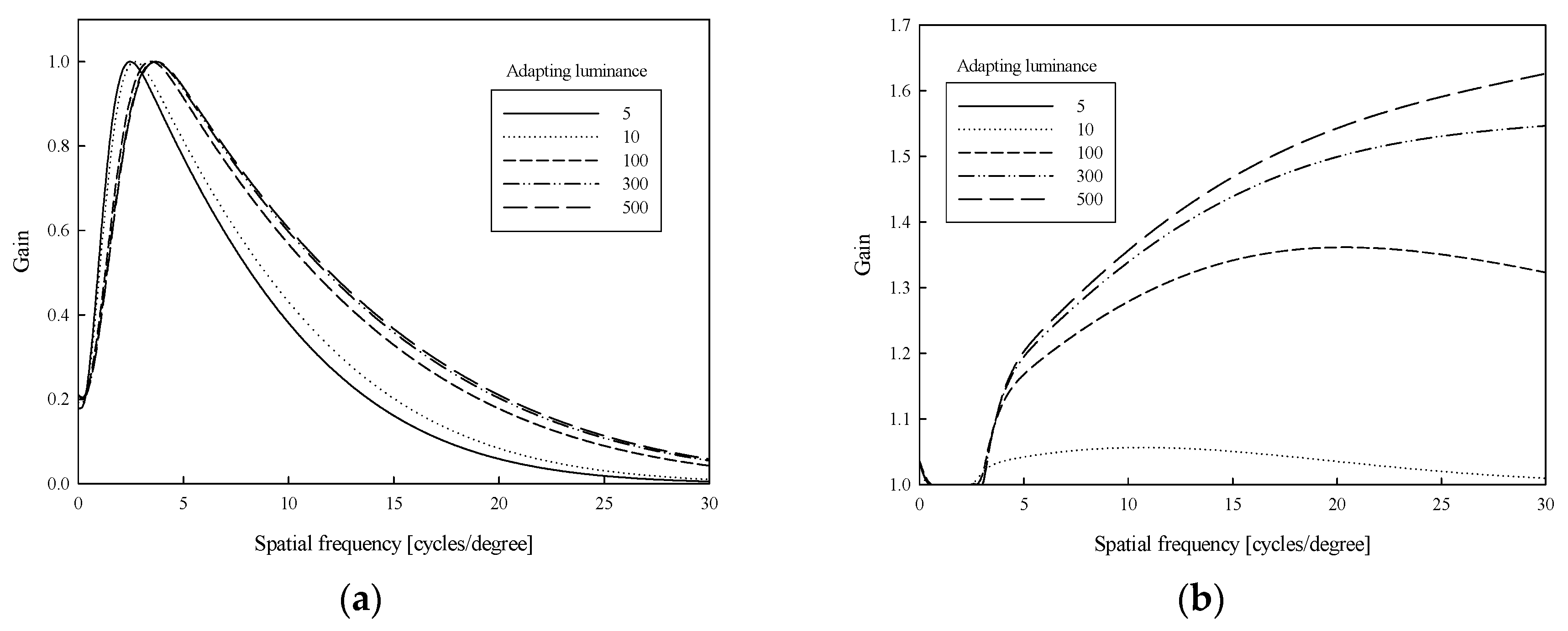Figure 4 represents proposed relative CSF curves and CSF sensitivity gain ($D{g}_{L_n}$) graphs. In Equation (15) and Equation (16), the final base and detail layer are composed through a linear interpolation between the two closest values $L_n$ of image $I$. This is based on a piecewise linear approximation of the previous fast bilateral filter. ${\sigma }_r$ is same as that of FBF for the same NB_SEGMENTS and ${\sigma }_s$ is set at a value of 2% of the image size. The CSF filter function can be designed for dim surround (< 5 $\mathrm{cd}/{\mathrm{m}}^2$). However, the sharpness compensation of HDR toning has been considered for more bright surround (> 5 $\mathrm{cd}/{\mathrm{m}}^2$) in which the minimum surround luminance, $L_{min}$ is set by 5 $\mathrm{cd}/{\mathrm{m}}^2$.

Processing steps of proposed method:

For n = 0 to NB_SEGMENTS

$$L_n=L_{min}+n\times \mathrm{segment}\_\mathrm{step}$$

(9)

$$I(L_n)=I\times g_{{\sigma }_r}(I-L_n)$$

(10)

$${\sigma }_{sn}={\sigma }_s\times (\arg \underset{f}{\max }CS{F}_{L_n}(f)/\arg \underset{f}{\max }CS{F}_{L_{min}}(f))$$

(11)

$$BaseLaye{r}_{L_n}=\mathrm{FFT}(I(L_n))\times \mathrm{FFT}(g_{{\sigma }_{sn}}(f))$$

(12)

$$D{g}_{L_n}(f)=(CS{F}_{L_n}(f)/CS{F}_{L_{min}}(f)-1)\times CS{F}_{L_n}(f)+1$$

(13)

$$DetailLaye{r}_L{}_n=D{g}_L{}_n(f)\times (\mathrm{FFT}(I(L_n))-BaseLaye{r}_L{}_n)$$

(14)

$$Bas{e}_n=Bas{e}_{n-1}+\mathrm{iFFT}(BaseLaye{r}_L{}_n)\times \mathrm{InterpolationWeight}(I,L_n)$$

(15)

$$Detai{l}_n=Detai{l}_{n-1}+\mathrm{iFFT}(DetailLaye{r}_L{}_n)\times \mathrm{InterpolationWeight}(I,L_n)$$

(16)

where $\mathrm{FFT}(·)$ and $\mathrm{iFFT}(·)$ are fast Fourier transform and inverse fast Fourier transform, respectively.

Figure 5 shows the proposed CSF-based base–detail separation and detail compensation processes in the 2-dimensional DFT domain. Through the proposed method, it is possible to perform selective sharpness improvement in the intensity segmented region in the DFT field without additional computation burden.

5. Simulations

In this section, we experimented with the rendering performance of the tone mapping method with the proposed CSF filter. In the experiments, we considered that the resolution of the experimental images was 30 pixels/degree (maximum range for spatial frequency) for the row and the column. Test images included the Macbeth color checker, and bright and noisy dark regions. As the viewer may feel less contrast sensitivity under the dim surround, we used test images of night indoor views.

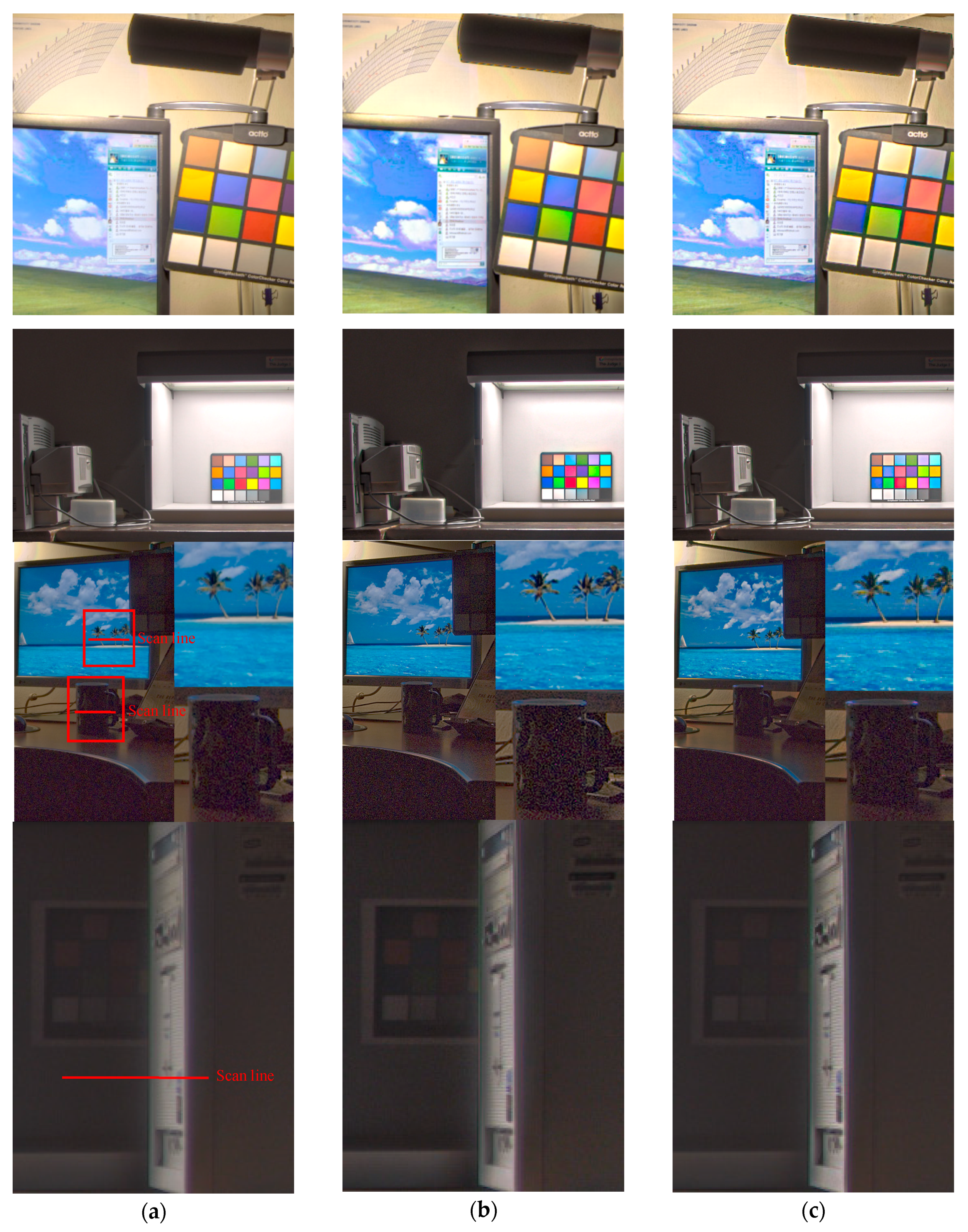
Figure 6 shows the HDR images rendered by comparable methods for evaluating the detail rendering performance. Figure 6a shows the rendered HDR images by the default Stevens adjust for detail layers in the iCAM06. Figure 6b shows rendered images with additional detail enhancement using the peak ratio of CSFs between bright and dim surrounds, as well as the Stevens adjust. The rendered images from the proposed model are shown in Figure 6c. It is easily confirmed that the proposed model is more sensitive than those of different methods around the edge and the object boundary. The detail enhancement is well-compared in color patches and in the background graph in first row images of Figure 6. Furthermore, to confirm contrast enhancement, we focused on the region around the lights. In the abrupt luminance change, such as object and light edges, the proposed method shows more clear edge lines when compared to the other methods.

Moreover, global enhancement using a CSF gain causes the color overshoots as shown in the abrupt edges of first and second row in Figure 6b. In addition, the sharpness enhancement and noise reduction compared to the result of global enhancement is shown in the upper and lower parts around the table in third row images of Figure 6. In order to compare the detail results, the edge renderings and noise differences in the detail area of the RGB channels were compared in Figure 7 for the scan line area of the bright and dark regions in the third and fourth rows in Figure 6b,c. In Figure 7a, the proposed method shows that the local contrast is equal to or better than the global method for the bright area, and simultaneously that the dark noise was reduced by far in the dark area in Figure 7b. In the proposed method of Figure 7c, the drastic change of intensity occurs in the transition region between background and object. As a result, the detail of the image is improved and the blur and noise are reduced.

We compare the proposed tone mapping method with the different methods for 15 test images. These tone mapping methods include a tone reproduction model considering lightness perception with characterizing the viewing environment and display, Reinhard (2012) [7], hybrid L1-L0 layer decomposition model, Liang (2018) [16], iCAM06 and the proposed method. User parameters of the simulated method are set as follows:

1.

Reinhard (2012)

Parameters are same as the environmental parameters of iCAM06 and the adapting luminance is 20 % of maximum luminance,

2.

Liang (2018)

B1 layer smoothness degree: ${\lambda }_1=0.3$

Detail layer smoothness degree: ${\lambda }_2={\lambda }_1\times 0.1$

B2 layer smoothness degree: ${\lambda }_3=0.1$

Gamma value: $\mathsf{\gamma }=2$,

3.

iCAM06

maximum luminance: $L_{max}=500$

Overall contrast: $p=0.75$

Surround adjustment: gamma value = 1

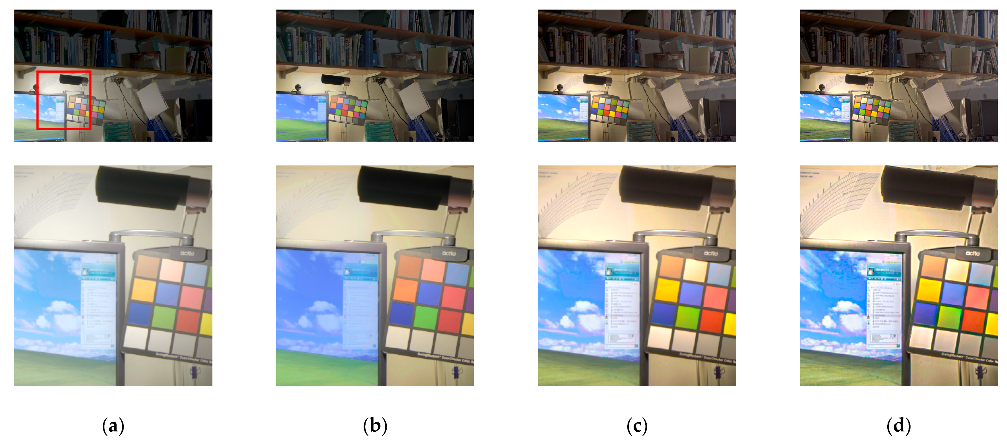
Figure 8 presents thumbnails of test images for various scenes. Figure 9, Figure 10 and Figure 11 show the comparison of tone mapping results on cropped regions. Figure 9 and Figure 10 present indoor situations which include the dark and bright regions. Each region is used to compare the details and colors with the different methods. In Figure 9, existing methods show lower contrast around the Macbeth color checker and lower detail of the drawing behind the monitor. On the other hand, the proposed method shows that the contrast and the detail of the drawing behind the monitor are clearly more enhanced than in other methods. In Figure 10, the printer region is compared in the aspect of detail expression and the light box region is used to compare the local contrast and colors. It can be seen that the details of the proposed method are well rendered. Figure 11 shows an outdoor scene with strong lightness and contrast. In the proposed method, the overall brightness is evenly improved and the detail of the wood is well represented. The area included in the background is clearly visible due to the improved contrast.

Subsequently, we perform the objective evaluation of three aspects, sharpness, HDR rendering quality and image quality using 15 HDR images in Figure 8. For the sharpness evaluation of each method, we select four kinds of sharpness metric, spectral and spatial sharpness (S3) [17], cumulative probability blur detection (CPBD) [18], local phase coherence-sharpness index (LPC-SI) [19] and just-noticeable blur (JNB) [20]. S3 perceives the local sharpness in image using spectral and spatial properties, and it was validated by comparison with sharpness maps generated by human subjects. CPBD is based on a probabilistic framework on the sensitivity of human blur perception at different contrasts. It is evaluated by taking into account the HVS response to blur distortions and the perceptual significance of the metric is validated through subjective experiments. LPC-SI evaluates image sharpness according to the degradation of LPC strength which is influenced by blur. JNB is defined as the threshold in which humans can perceive blurriness around an edge shown in a contrast higher than the just-noticeable difference. JNB considers the response of the HVS to sharpness at different contrast levels. The above methods do not require a reference to evaluate. The higher score of each method represents the properly sharpened image. In particular, S3, CPBD, and JBN methods are based on HVS simulation and the results of each method well-reflect the visual characteristics.

Table 1. Comparison with sharpness scores.

	Reinhard(2012)	Liang(2018)	iCAM06	Proposed
S3	0.399	0.421	0.432	0.565
CPBD	0.522	0.509	0.516	0.573
LPC-SI	0.921	0.928	0.932	0.951
JNB	15.93	16.05	15.90.	18.58

shows the average sharpness score of four tone mapping methods. The proposed method has higher tone mapping than other methods for each sharpness method.

In

Table 2. Comparison with TMQI scores.

	Reinhard(2012)	Liang(2018)	iCAM06	Proposed
TMQI	0.839	0.826	0.866	0.868
Fidelity	0.874	0.870	0.898	0.886
Naturalness	0.264	0.204	0.361	0.387

, we compare a rendered HDR image quality in each method using the tone mapped image quality index (TMQI) which is an objective quality assessment metric for tone-mapped images [21]. TMQI consists of a multiscale signal fidelity measure and a statistical naturalness measure. The fidelity measure extracts the structural information from the visibility to estimate the perceptual quality. It calculates the cross-correlation between HDR and LDR image pairs, and uses the pyramid image to evaluate the visibility of image detail according to the distance between the image and observer. The naturalness measure evaluates the brightness and contrast of the tone mapped image. The TMQI score is the weighted sum of the fidelity measure and naturalness measure. Each measure ranges from 0 to 1 and the larger score indicates better quality in image rendering. Our test result is shown in Table 2. The fidelity measurement uses local standard deviations for the structural information. When the structural information of the tone mapped image is close to that of input HDR image, the fidelity score is higher. However, the proposed method compensates for the local details using relative CSF gains in frequency domain. Therefore, the local standard variations of the proposed method are higher than those of the iCAM06. As a result, the fidelity score of the proposed method is slightly lower than iCAM06, but the naturalness score is better than those of other methods. The final TMQI score shows that the proposed method has the highest score.

In

Table 3. Comparison with PIQE scores.

	Reinhard(2012)	Liang(2018)	iCAM06	Proposed
PIQE	31.37	28.04	25.79	22.71

, we compare image quality for each method using a no-reference perception-based image quality evaluator (PIQE). The PIQE is an unsupervised algorithm which does not use any statistical learning to evaluate image quality. The PIQE extracts local features to estimate image quality. Each feature is classified according to the degree of distortion and assigned a score. The score range is between 0 to 100 and lower values represent better quality [22]. From the overall assessment based on the qualitative comparisons, we confirm that the proposed method produces reasonable detail enhancement in the dark region and good HDR rendering results.

6. Conclusions

The iCAM06 tends to reduce the sharpness of dim surround due to the fixed edge-stopping function of the FBF in iCAM06. This paper proposes the base–detail separation and frequency segmented detail compensation using the relative CSF gain for different frequencies. We designed a layer separation filter which can be applied to the base–detail separation and sharpness enhancement locally in the aspect of the contrast sensitivity. To compare objective evaluations for the sharpness enhancement, HDR rendering quality and image quality, we used four sharpness metrics, TMQI and PIQE, respectively. The experimental results show that the iCAM06 using the proposed method has better performance than the existing methods.