Blind Image Deconvolution Algorithm Based on Sparse Optimization with an Adaptive Blur Kernel Estimation


Abstract
1. Introduction
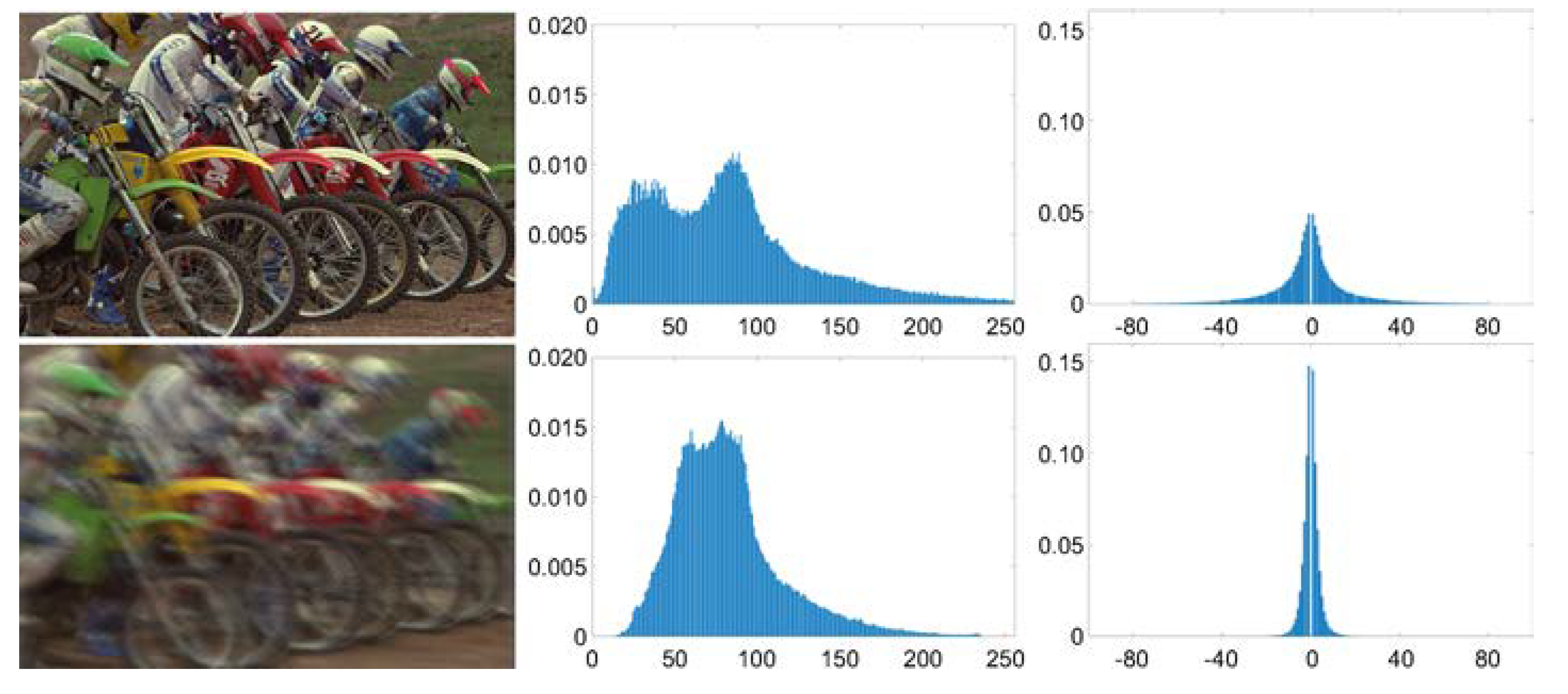
- An image prior based on nonzero measurement on four orientations of the image gradient domain is proposed. The image histogram charts show that the frequency of nonzero values in the gradient domain of a blurry image is far more than that in a clear one, and the nonzero measurement is suitable for a constraint for image deblurring. The solution for the cost function with the proposed image prior is also analyzed and discussed.
- The blur kernel is obtained under a ridge regularization on the PSF because the measurements on an image are enough to estimate the blur kernel in the maximum a posteriori (MAP) framework. During the optimization, we propose a solution based on a conjugate gradient method combined with Newton’s method; this solution could prevent us from calculating the inversion of a Hessian matrix and solve the cost function efficiently.
- Considering the statistical features of natural images, we presented a non-blind image deconvolution algorithm by applying the concept of hyper-Laplacian distribution-based prior. Its target image is constrained by an quasi-norm in the cost function. We analyze and discuss the solutions for different values.
- We tested our method on both simulated motion blurs and atmospheric turbulence blurs in real-life applications. In addition, we comparatively analyzed our method, in terms of the cost durations, estimated accuracy of the blur kernels, and quality assessment of the restored images, and adopted several approaches related to blur removal.
2. Materials and Methods
2.1. Image Prior and Our Method’s Framework
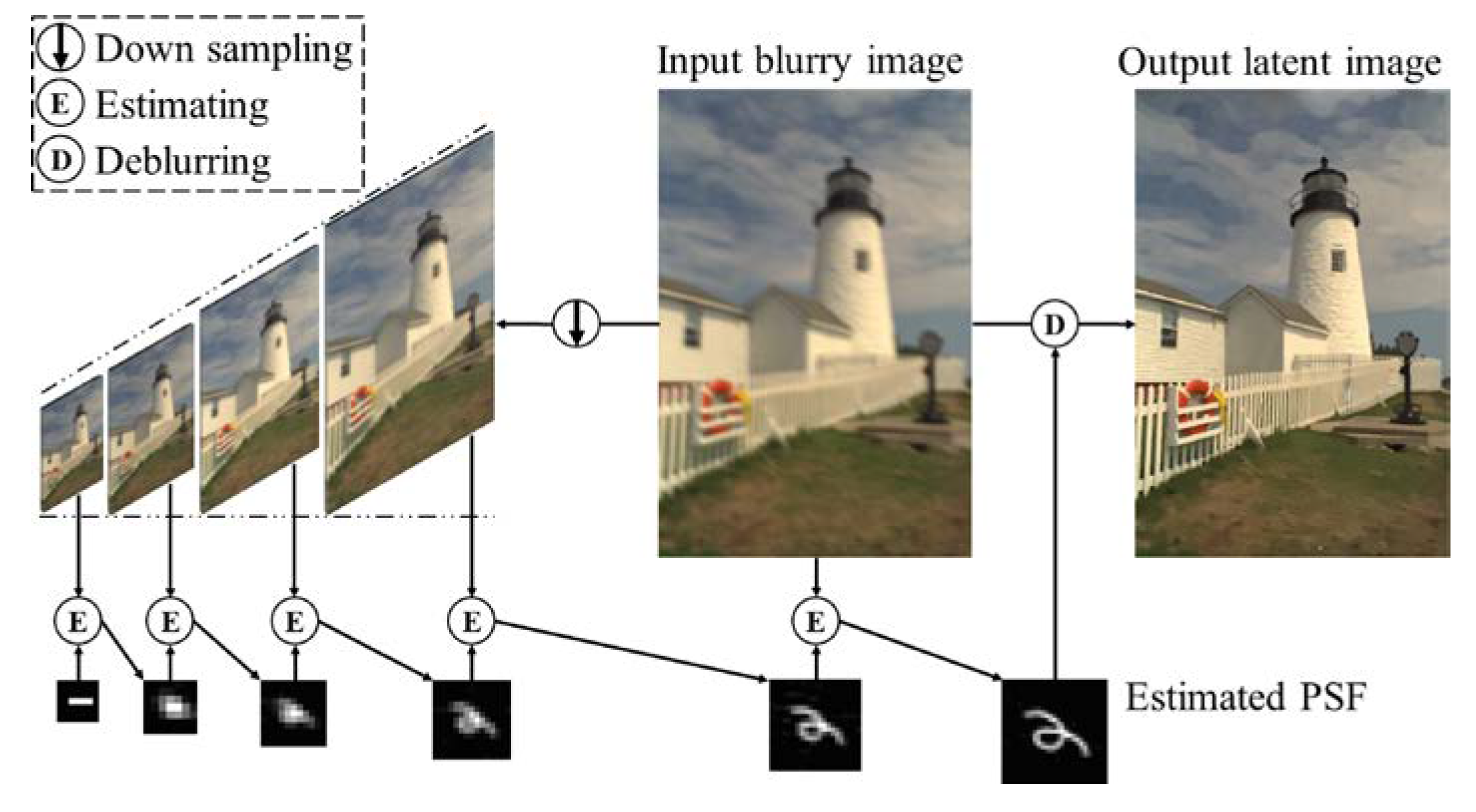
2.2. Estimation of Blur Kernel and the Intermediate Latent Image
2.2.1. Solve with a Given
2.2.2. Solve with a given
2.3. Image Restoration
2.4. Smooth the Image Boundaries
3. Results and Discussion
3.1. Comparisons of Blur Kernel Estimations
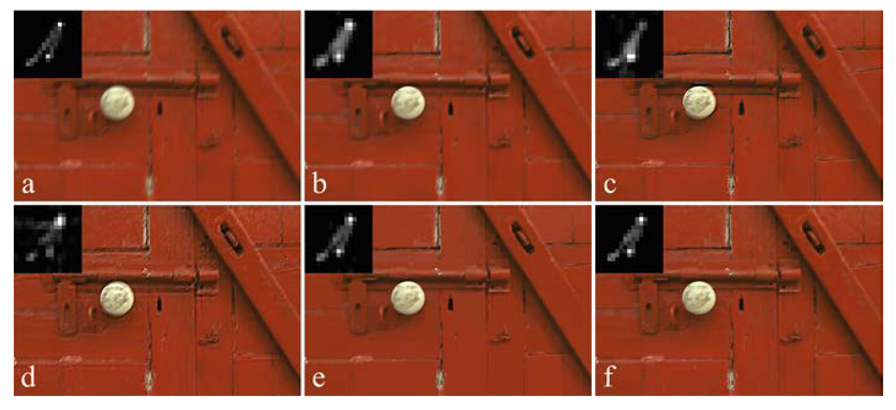
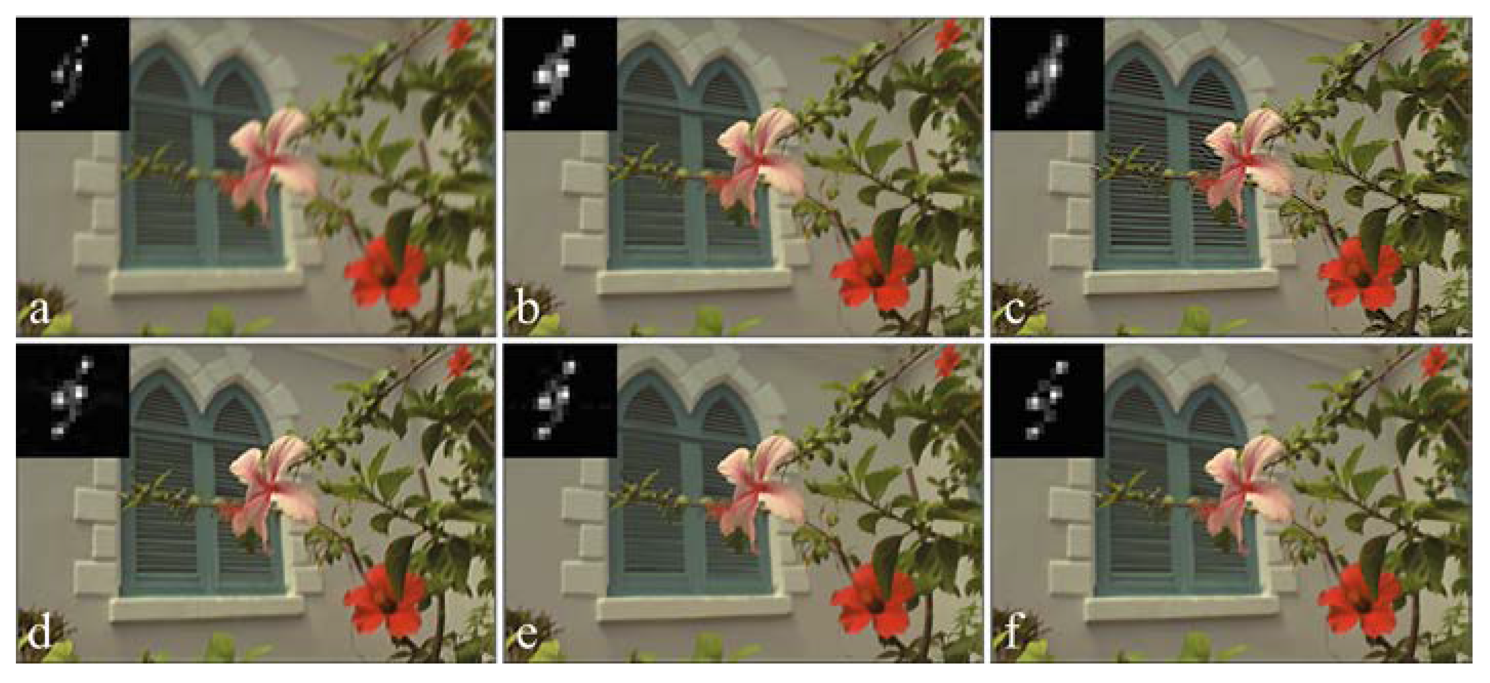
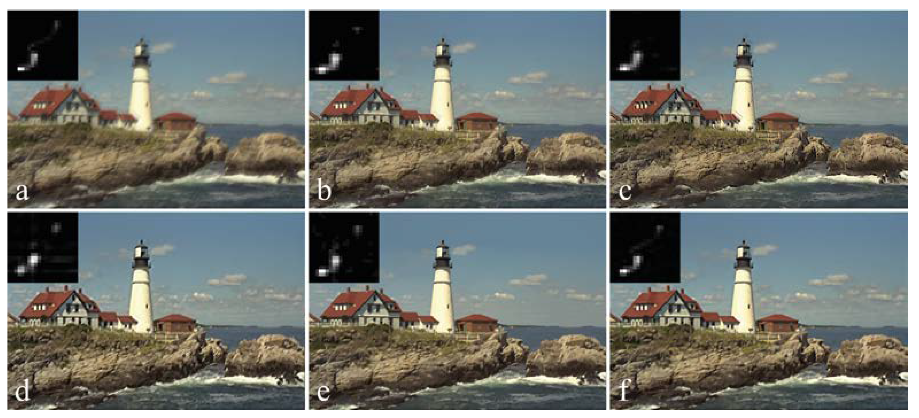
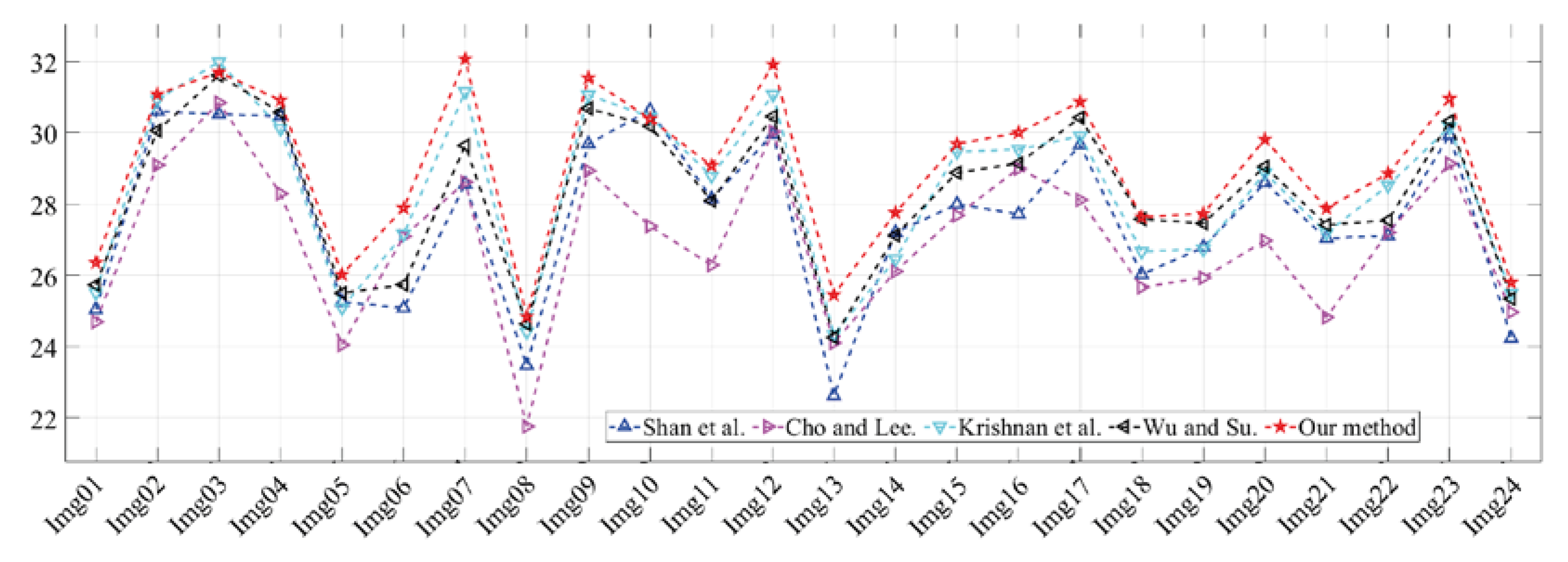
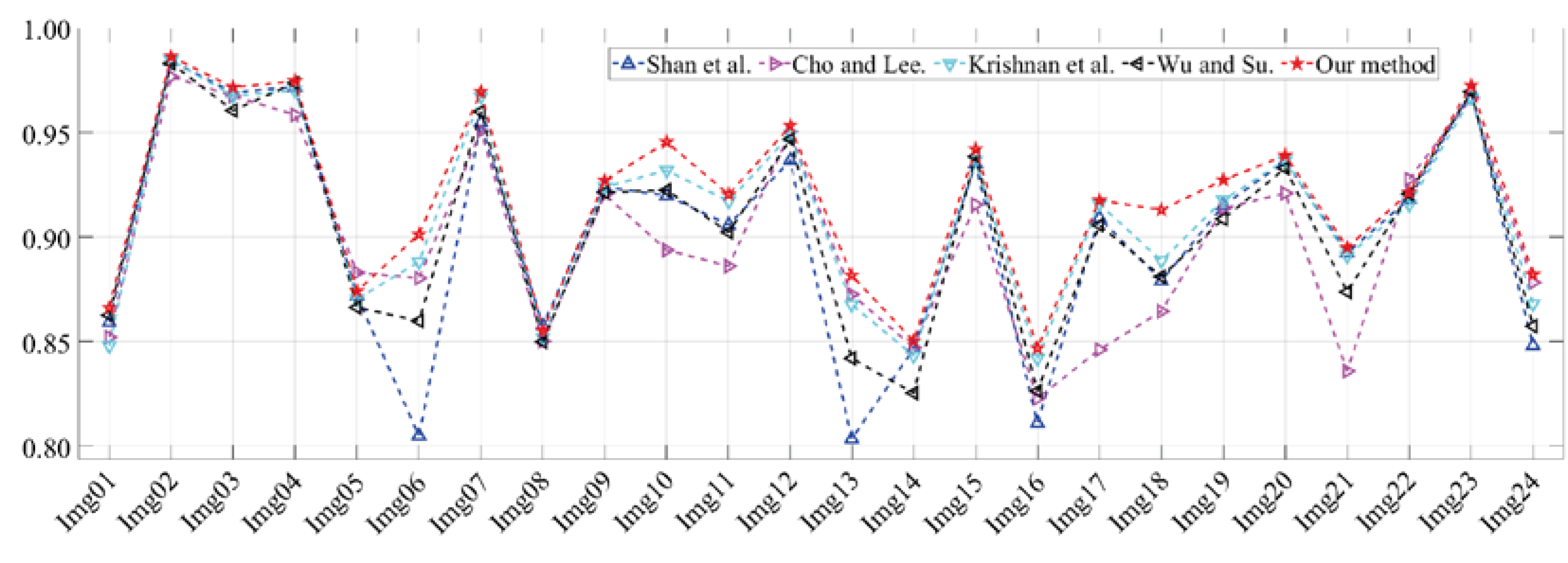
3.2. Comparison of Deblurring Results.
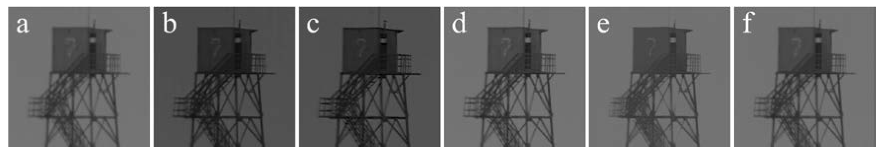
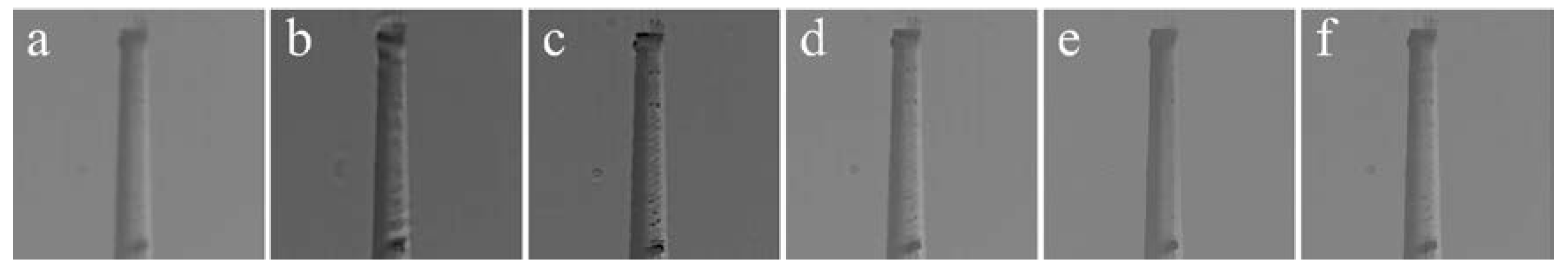
3.3. Real-Life Applications
4. Conclusions
Author Contributions
Funding
Acknowledgments
Conflicts of Interest
References
- El-Sallam, A.A.; Boussaid, F. Spectral-based blind image restoration method for thin TOMBO imagers. Sensors 2008, 8, 6108–6124. [Google Scholar] [CrossRef]
- Zhang, W.; Quan, W.; Guo, L. Blurred star image processing for star sensors under dynamic conditions. Sensors 2012, 12, 6712–6726. [Google Scholar] [CrossRef]
- Manfredi, M.; Bearman, G.; Williamson, G.; Kronkright, D.; Doehne, E.; Jacobs, M.; Marengo, E. A new quantitative method for the non-invasive documentation of morphological damage in paintings using RTI surface normals. Sensors 2014, 14, 12271–12284. [Google Scholar] [CrossRef]
- Luan, S.; Xie, S.; Wang, T.; Hao, X.; Yang, M.; Li, Y. A Space-Variant Deblur Method for Focal-Plane Microwave Imaging. Appl. Sci. 2018, 8, 2166. [Google Scholar] [CrossRef]
- Zhang, H.; Yuan, B.; Dong, B.; Jiang, Z. No-Reference Blurred Image Quality Assessment by Structural Similarity Index. Appl. Sci. 2018, 8, 2003. [Google Scholar] [CrossRef]
- Ali, U.; Mahmood, M.T. Analysis of blur measure operators for single image blur segmentation. Appl. Sci. 2018, 8, 807. [Google Scholar] [CrossRef]
- Dash, R.; Majhi, B. Motion blur parameters estimation for image restoration. Optik 2014, 125, 1634–1640. [Google Scholar] [CrossRef]
- Jalobeanu, A.; Blanc-Feraud, L.; Zerubia, J. An adaptive Gaussian model for satellite image deblurring. IEEE Trans. Image Process. 2004, 13, 613–621. [Google Scholar] [CrossRef] [PubMed]
- Kumar, A.; Paramesran, R.; Lim, C.-L.; Dass, S.C. Tchebichef moment based restoration of Gaussian blurred images. Appl. Opt. 2016, 55, 9006–9016. [Google Scholar] [CrossRef] [PubMed]
- Yin, H.; Hussain, I. Independent component analysis and nongaussianity for blind image deconvolution and deblurring. Integr. Comput. Aided Eng. 2008, 15, 219–228. [Google Scholar] [CrossRef]
- Saleh, A.K.; Arashi, M.; Kibria, B.G. Theory of Ridge Regression Estimation with Applications; John Wiley & Sons: Hoboken, NJ, USA, 2019; ISBN 978-1-118-64461-4. [Google Scholar]
- Field, D.J. What is the Goal of Sensory Coding? Neural Comput. 1994, 6, 559–601. [Google Scholar] [CrossRef]
- Weiss, Y.; Freeman, W.T. What makes a good model of natural images? In Proceedings of the 2007 IEEE Conference on Computer Vision and Pattern Recognition, Minneapolis, MN, USA, 17–22 June 2007; pp. 1–8. [Google Scholar]
- Fergus, R.; Singh, B.; Hertzmann, A.; Roweis, S.T.; Freeman, W.T. Removing camera shake from a single photograph. ACM Trans. Graph. 2006, 25, 787–794. [Google Scholar] [CrossRef]
- Levin, A.; Fergus, R.; Durand, F.; Freeman, W.T. Image and depth from a conventional camera with a coded aperture. ACM Trans. Graph. 2007, 26, 70-es. [Google Scholar] [CrossRef]
- Joshi, N.; Zitnick, C.L.; Szeliski, R.; Kriegman, D.J. Image deblurring and denoising using color priors. In Proceedings of the 2009 IEEE Conference on Computer Vision and Pattern Recognition, Miami, FL, USA, 20–25 June 2009; pp. 1550–1557. [Google Scholar]
- Wang, Y.; Yang, J.; Yin, W.; Zhang, Y. A New Alternating Minimization Algorithm for Total Variation Image Reconstruction. SIAM J. Imaging Sci. 2008, 1, 248–272. [Google Scholar] [CrossRef]
- Xu, L.; Jia, J. Two-Phase Kernel Estimation for Robust Motion Deblurring. In Computer Vision—ECCV 2010. ECCV 2010; Daniilidis, K., Maragos, P., Paragios, N., Eds.; Heraklion: Crete, Greece; Springer: Berlin/Heidelberg, Germany, 2010; Volume 6311, pp. 157–170. [Google Scholar]
- Pan, J.; Sun, D.; Pfister, H.; Yang, M.-H. Blind Image Deblurring Using Dark Channel Prior. In Proceedings of the 2016 IEEE Conference on Computer Vision and Pattern Recognition (CVPR), Las Vegas, NV, USA, 27–30 June 2016; pp. 1628–1636. [Google Scholar]
- Yang, H.; Su, X.; Ju, C.; Wu, S. Efficient Self-Adaptive Image Deblurring Based on Model Parameter Optimization. In Proceedings of the 2018 IEEE 3rd International Conference on Image, Vision and Computing (ICIVC), Chongqing, China, 27–29 June 2018; pp. 384–388. [Google Scholar]
- Zhu, S.C.; Mumford, D.B. Prior learning and Gibbs reaction-diffusion. IEEE Trans. Pattern Anal. Mach. Intell. 1997, 19, 1236–1250. [Google Scholar] [CrossRef]
- Roth, S.; Black, M.J. Fields of Experts: A framework for learning image priors. In Proceedings of the 2005 IEEE Computer Society Conference on Computer Vision and Pattern Recognition (CVPR’05), San Diego, CA, USA, 20–25 June 2005; Volume 2, pp. 860–867. [Google Scholar]
- Raj, A.; Zabih, R. A graph cut algorithm for generalized image deconvolution. In Proceedings of the Tenth IEEE International Conference on Computer Vision (ICCV’05) Volume 1, Beijing, China, 17–21 October 2005; Volume 2, pp. 1048–1054. [Google Scholar]
- Schuler, C.J.; Burger, C.H.; Harmeling, S.; Scholkopf, B. A Machine Learning Approach for Non-blind Image Deconvolution. In Proceedings of the 2013 IEEE Conference on Computer Vision and Pattern Recognition, Portland, OR, USA, 23–28 June 2013; pp. 1067–1074. [Google Scholar]
- Zhang, K.; Zuo, W.; Gu, S.; Zhang, L. Learning Deep CNN Denoiser Prior for Image Restoration. In Proceedings of the 2017 IEEE Conference on Computer Vision and Pattern Recognition, Honolulu, HI, USA, 21–26 July 2017; pp. 2808–2817. [Google Scholar]
- Snyder, W.E.; Qi, H. Machine Vision; Cambridge University Press: New York, NY, USA, 2010; ISBN 9780521169813. [Google Scholar]
- Levin, A.; Weiss, Y.; Durand, F.; Freeman, W.T. Understanding and evaluating blind deconvolution algorithms. In Proceedings of the 2009 IEEE Conference on Computer Vision and Pattern Recognition, Miami, FL, USA, 20–25 June 2009; pp. 1964–1971. [Google Scholar]
- Levin, A.; Weiss, Y.; Durand, F.; Freeman, W.T. Efficient marginal likelihood optimization in blind deconvolution. In Proceedings of the 2011 IEEE Conference on Computer Vision and Pattern Recognition, Providence, RI, USA, 20–25 June 2011; pp. 2657–2664. [Google Scholar]
- Miao, L.; Qi, H. A Blind Source Separation Perspective on Image Restoration. In Proceedings of the 2007 IEEE Conference on Computer Vision and Pattern Recognition, Minneapolis, MN, USA, 17–22 June 2007; pp. 1–7. [Google Scholar]
- Mathews, J.H.; Fink, K.D. Numerical Methods Using MATLAB, 4th ed.; Pearson Prentice Hall Press: Upper Saddle River, NJ, USA, 2004; ISBN 97871219074. [Google Scholar]
- Abramowitz, M. Handbook of Mathematical Functions: With Formulas, Graphs, and Mathematical Tables; Dover Publications: Mineola, New York, USA, 1974; ISBN 0486612724. [Google Scholar]
- Wright, S.J.; Nowak, R.D.; Figueiredo, M.A. Sparse reconstruction by separable approximation. IEEE Trans. Signal Process. 2009, 57, 2479–2493. [Google Scholar] [CrossRef]
- Liu, R.; Jia, J. Reducing boundary artifacts in image deconvolution. In Proceedings of the 2008 15th IEEE International Conference on Image Processing, San Diego, CA, USA, 12–15 October 2008; pp. 505–508. [Google Scholar]
- Franzen, R. Kodak Lossless True Color Image Suite, Kodak PhotoCD PCD0992 image samples in PNG file format. Available online: http://r0k.us/graphics/kodak/ (accessed on 1 January 2020).
- Shan, Q.; Jia, J.; Agarwala, A. High-quality motion deblurring from a single image. ACM Trans. Graph. 2008, 27, 1–10. [Google Scholar] [CrossRef]
- Cho, S.; Lee, S. Fast motion deblurring. ACM Trans. Graph. 2009, 28, 1–8. [Google Scholar] [CrossRef]
- Krishnan, D.; Tay, T.; Fergus, R. Blind deconvolution using a normalized sparsity measure. In Proceedings of the 2011 IEEE Conference on Computer Vision and Pattern Recognition, Providence, RI, USA, 20 June 2011; pp. 233–240. [Google Scholar]
- Wu, J.; Su, X. Method of Image Quality Improvement for Atmospheric Turbulence Degradation Sequence Based on Graph Laplacian Filter and Nonrigid Registration. Math. Prob. Eng. 2018, 2018, 1–15. [Google Scholar] [CrossRef]
- Hore, A.; Ziou, D. Image Quality Metrics: PSNR vs. SSIM. In Proceedings of the 20th International Conference on Pattern Recognition, Istanbul, Turkey, 23–26 August 2010; pp. 2366–2369. [Google Scholar]
- Moorthy, A.K.; Bovik, A.C. A two-step framework for constructing blind image quality indices. IEEE Signal Process. Lett. 2010, 17, 513–516. [Google Scholar] [CrossRef]
- Liu, L.; Liu, B.; Huang, H.; Bovik, A.C. No-reference image quality assessment based on spatial and spectral entropies. Signal Process. Image Commun. 2014, 29, 856–863. [Google Scholar] [CrossRef]


| PSF | Number | (a) | (b) | (c) | (d) | (e) | (f) | (g) | (h) |
|---|---|---|---|---|---|---|---|---|---|
| Size | |||||||||
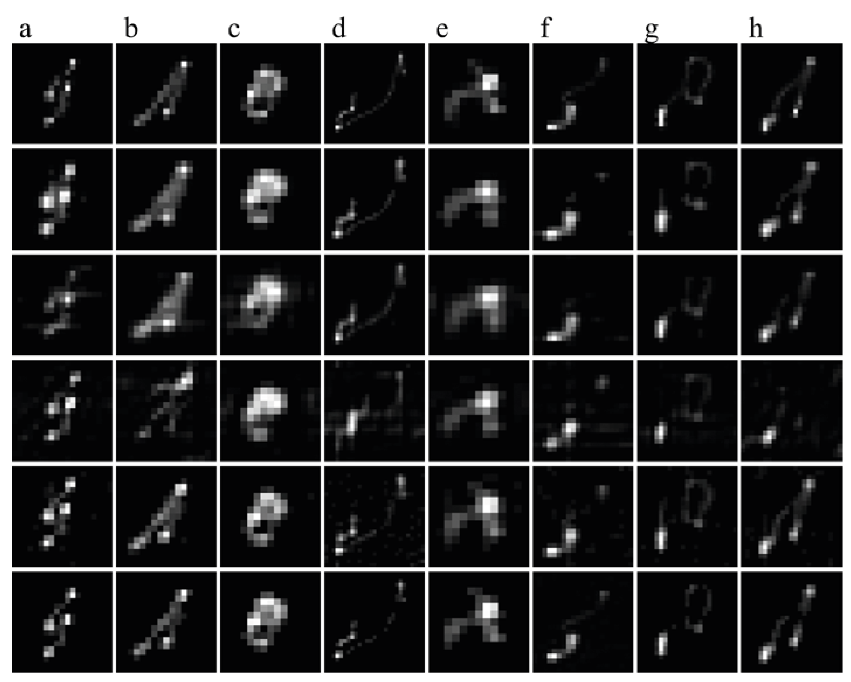
| Method in [35] | Duration | 64.572 | 63.431 | 56.714 | 81.508 | 50.356 | 67.938 | 69.447 | 74.999 |
| MSE | 0.6182 | 0.2592 | 0.2259 | 0.1062 | 0.6942 | 0.2656 | 0.1457 | 0.0975 | |
| Method in [36] | Duration | 6.9690 | 6.9370 | 6.8580 | 7.5930 | 6.1690 | 7.0620 | 7.0930 | 7.3120 |
| MSE | 0.4893 | 0.3763 | 0.3722 | 0.0977 | 0.7499 | 0.2036 | 0.0867 | 0.1339 | |
| Method in [37] | Duration | 95.979 | 56.916 | 35.043 | 211.07 | 25.636 | 110.29 | 131.32 | 143.96 |
| MSE | 0.6249 | 0.7617 | 0.2892 | 0.3221 | 0.4817 | 0.3404 | 0.1711 | 0.4252 | |
| Method in [38] | Duration | 71.577 | 70.950 | 65.525 | 126.08 | 58.953 | 77.165 | 110.45 | 119.04 |
| MSE | 0.5624 | 0.3650 | 0.1807 | 0.1364 | 0.2374 | 0.2312 | 0.1012 | 0.1525 | |
| Proposed method | Duration | 14.702 | 14.327 | 13.796 | 28.076 | 13.171 | 18.061 | 21.624 | 21.653 |
| MSE | 0.4823 | 0.1540 | 0.1024 | 0.0675 | 0.1110 | 0.1161 | 0.0627 | 0.0821 |
| Test Images | FRIQA | Method in [35] | Method in [36] | Method in [37] | Method in [38] | Proposed Method |
|---|---|---|---|---|---|---|
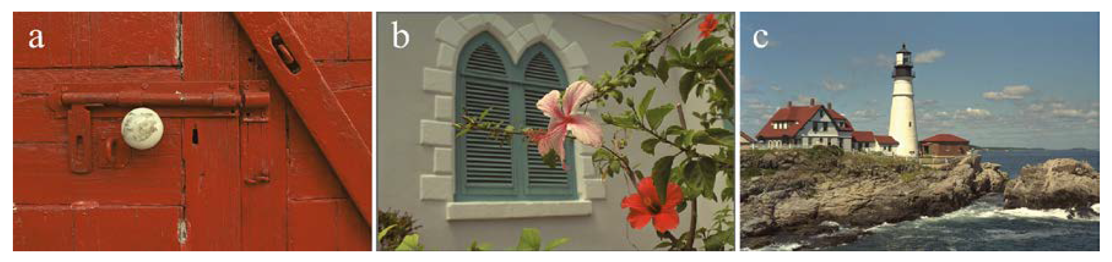
| “RedDoor.png” | PSNR | 28.660 | 26.126 | 27.126 | 28.633 | 28.986 |
| SSIM | 0.9751 | 0.9570 | 0.9660 | 0.9764 | 0.9787 | |
| “Flowers.png” | PSNR | 27.411 | 26.082 | 27.429 | 27.826 | 28.240 |
| SSIM | 0.9049 | 0.9120 | 0.9173 | 0.9122 | 0.9177 | |
| “Lighthouse.png” | PSNR | 25.197 | 24.297 | 24.887 | 25.577 | 25.841 |
| SSIM | 0.8816 | 0.8724 | 0.8651 | 0.8791 | 0.8867 |
| Test Images | NRIQA | Method in [35] | Method in [36] | Method in [37] | Method in [38] | Proposed Method |
|---|---|---|---|---|---|---|
| “Tower.bmp” | BIBQ | 46.347 | 38.829 | 41.496 | 39.855 | 37.293 |
| SSEQ | 37.831 | 46.839 | 40.268 | 36.637 | 35.693 | |
| “Chimney.bmp” | BIBQ | 57.800 | 52.974 | 58.437 | 52.889 | 51.953 |
| SSEQ | 69.902 | 52.127 | 59.659 | 49.884 | 33.326 | |
| “Pole.bmp” | BIBQ | 52.357 | 45.612 | 46.507 | 45.246 | 41.586 |
| SSEQ | 45.693 | 52.588 | 44.672 | 39.171 | 37.514 |
© 2020 by the authors. Licensee MDPI, Basel, Switzerland. This article is an open access article distributed under the terms and conditions of the Creative Commons Attribution (CC BY) license (http://creativecommons.org/licenses/by/4.0/).
Share and Cite
Yang, H.; Su, X.; Chen, S. Blind Image Deconvolution Algorithm Based on Sparse Optimization with an Adaptive Blur Kernel Estimation. Appl. Sci. 2020, 10, 2437. https://doi.org/10.3390/app10072437
Yang H, Su X, Chen S. Blind Image Deconvolution Algorithm Based on Sparse Optimization with an Adaptive Blur Kernel Estimation. Applied Sciences. 2020; 10(7):2437. https://doi.org/10.3390/app10072437
Chicago/Turabian StyleYang, Haoyuan, Xiuqin Su, and Songmao Chen. 2020. "Blind Image Deconvolution Algorithm Based on Sparse Optimization with an Adaptive Blur Kernel Estimation" Applied Sciences 10, no. 7: 2437. https://doi.org/10.3390/app10072437
APA StyleYang, H., Su, X., & Chen, S. (2020). Blind Image Deconvolution Algorithm Based on Sparse Optimization with an Adaptive Blur Kernel Estimation. Applied Sciences, 10(7), 2437. https://doi.org/10.3390/app10072437