Automatic Classification of Web Images as UML Static Diagrams Using Machine Learning Techniques

Featured Application

The tool presented in this paper is useful in improving the effectiveness of common web search engines like Google Images. The tool is also useful for searching private repositories in an organization, when metadata are not available. The development of a UML-oriented information retrieval tool can easily be expanded to applications in different domains.

Abstract

Our purpose in this research is to develop a method to automatically and efficiently classify web images as Unified Modeling Language (UML) static diagrams, and to produce a computer tool that implements this function. The tool receives a bitmap file (in different formats) as an input and communicates whether the image corresponds to a diagram. For pragmatic reasons, we restricted ourselves to the simplest kinds of diagrams that are more useful for automated software reuse: computer-edited 2D representations of static diagrams. The tool does not require that the images are explicitly or implicitly tagged as UML diagrams. The tool extracts graphical characteristics from each image (such as grayscale histogram, color histogram and elementary geometric forms) and uses a combination of rules to classify it. The rules are obtained with machine learning techniques (rule induction) from a sample of 19,000 web images manually classified by experts. In this work, we do not consider the textual contents of the images. Our tool reaches nearly 95% of agreement with manually classified instances, improving the effectiveness of related research works. Moreover, using a training dataset 15 times bigger, the time required to process each image and extract its graphical features (0.680 s) is seven times lower.

1. Introduction

The Unified Modeling Language (UML) was born in the early 1990s with the intent of merging various traditions of software modeling into a single graphical, general-purpose language. As its three original authors posed it, the purpose of the UML was to provide a standard way to specify, visualize, document, modify and construct the design of a (software) system [1]. The Object Management Group (OMG) soon started a standardization process that produced the first versions of the language specification in the late 1990s (UML 1.1 in 1997). After several minor revisions, UML 1.x was replaced by UML 2.x in 2005; the latest versions are UML 2.5 (released in May 2015) and 2.5.1 (released in December 2017 [2]). During the past two decades, the UML has been progressively adopted by the software industry, so that it has become a de facto standard, usually taught in undergraduate university courses in software engineering, and with a plethora of scientific journals and conferences around it.

Model Driven Engineering (MDE) (also called Model Driven Development, MDD) was a subsequent OMG initiative, whose central idea was to shift the emphasis in the software development process from source code to software models [3,4]: planning, estimating, reuse, maintenance, production, simulation and so on. This initiative is of great importance for a software development process based on model transformations to be truly iterative: integration and coherence of all phases of development, models synchronized at all levels, etc. The application of MDE is growing in the development of software systems (or hardware–software combinations), as long as new methodologies and tools are available to manipulate software models. In particular, MDE has also moved the center of interest in the area of software reuse towards models and associated modeling artifacts, instead of sheer code. However, a practical adoption of fruitful reuse practices demands specific tools to classify and retrieve software models, which is not a simple task, due to the fact that models and diagrams are not sequential text-structures, but multidimensional artifacts made of a combination of text and logical relationships [5,6].

UML defines a variety of diagram types that inherit and develop different notations that have existed for years, such as entity–relationship diagrams and statecharts. Diagrams are graphs made up of nodes of various forms (rectangles, ellipses, etc.), typically with some structured text inside, and labeled arcs with terminators such as arrowheads. Diagrams may be static or dynamic (with several subtypes each), representing different aspects or views of a software system. Essentially, static diagrams represent the structure of the system and its parts, and dynamic diagrams represent its temporal evolution and behavior. There are different kinds of models in software engineering: analysis and design models, structural and behavioral models and others, so it is of major importance to understand the meaning of each kind of model, how they are related and how they evolve [7]. A system’s model is usually represented by a combination of various diagram types that provide different architectural views to achieve a comprehensive understanding of the system. The most widely used diagram type in software development is the class diagram, which is a kind of static diagram. It is typically used at different levels of abstraction to represent, for example, the information model or logical view of the system (high level) or the structure of the implementation code (low level).

UML diagrams can be produced through a variety of means, from simple drawing tools to fully developed computer assisted software engineering (CASE) tools that can check the syntax and coherence between diagrams, and even produce executable code. Models can then be stored in public or proprietary repositories that are conformant to the UML metamodel and can offer their own classification and retrieval facilities to manage them and, in particular, reuse their contents. These repositories are useful both for academic research and for industrial developments. However, even if there exists an OMG standard format to store models (XMI, XML Metadata Interchange [8]), the compatibility of many commercial tools is not assured. Moreover, it is very common to insert the diagrams in software documentation in a purely graphical format (bitmap images), where explicit compliance with the UML metamodel is lost. The large amount of these kinds of images on the web makes the possibility to retrieve their modeling information for reuse purposes very interesting. However, this task presents notable difficulties broadly pertaining to these two categories:

• Image retrieval. In order to achieve an effective retrieval, images should be conveniently tagged so that web crawlers can classify and index them, but this rarely happens. Therefore, images must be located based on their surrounding text, which can refer (or not refer) to the image contents, and can provide (or not provide) the necessary or desired search arguments. This implies that a lot of noise (lack of precision) or a lot of silence (lack of recall) is usually obtained.
• Information extraction. Once the bitmap image is retrieved, it must be converted to a UML-compliant format in order to extract its modeling information. This task requires the use of artificial vision techniques, whose effectiveness is highly dependent on the quality of the image and embedded text, its level of compliance to the UML specification (very often informally followed), and so on.

In this work we focus on the first category of problems, leaving the second category for future research. Our approach to improve the precision and recall of the retrieval of images representing UML diagrams is based on well-known machine learning techniques, as explained later: we had a computer tool learn from a previous human-made classification of images. Therefore, our work’s intent is not to improve machine learning techniques, but rather to devise a novel application to the field of web image retrieval, with huge potential for software reuse.

The rest of the paper is structured as follows. Section 2 further develops the motivation and expected benefits from this research, and gives an outline of the method we have developed. Section 3 reviews the related work on automatic recognition of UML diagrams, either using machine learning techniques or not. Section 4 reports the main graphical characteristics of images that can be effectively used to classify them as diagrams, and describes our method to identify straight lines and rectangles, which is key to obtain results with computational efficiency. Section 5 shows that a simple combination of metrics is insufficient to discriminate between diagrams and non-diagrams, thus justifying the use of machine learning techniques to build an easily computable discrimination function. Section 6 explains the construction of the automatic rule-based classifier that solves the problem of computing the concrete intervals for each metric and the combination of metrics, using well-known machine learning techniques (rule induction). Section 7 describes the experiments and results we obtained in precision, recall and accuracy, also showing some examples of individual rules that build up the automatic classifier. Section 8 presents the i2m classification tool and how we plan to develop it in the future. Finally, Section 9 offers some concluding remarks.

This paper is an extended version of a previous paper presented at the 4th Spanish Conference in Information Retrieval [9]. That version was constrained due to its rather short length, and the authors could not explain in sufficient detail the grounds of our contribution. In this version, we display a richer context about UML, MDD, class diagrams and model repositories (Section 1), as well as a much more thorough exposition of the results of previous works from other researchers (Section 3). We also give a new in-depth explanation of the principles of rectangle identification (Section 4) and an explanation of classification functions in a hyperspace of features that justifies the reasonableness of the rule induction approach (Section 5). The description of the rule induction process was enriched with the mathematical formulation of the problem in terms of search-based software engineering, and with a fully detailed textual and graphical explanation of the two stages of the process, namely rule inference and rule application (Section 6). Finally, a comparison with previous research was completed with detailed numerical data that support our claim about the better performance of our work (Section 9).

2. Motivation and Outline of Method

Our purpose in this research is to develop a method for the automatic and efficient classification of web images as UML static diagrams, and to produce a computer tool that implements this function. The tool receives a bitmap file (in different formats) as an input and indicates whether the image corresponds to a diagram.

This tool is useful as long as it improves the effectiveness of common image search engines (measured as accuracy, i.e., percentage of agreement between automatic and manual classification). For example, Google currently offers the possibility of an advanced search of images with a filter set to “line drawing”. Using this filter, a generic search argument such as “control system” provides nearly no results that can be recognized as software engineering diagrams. Simply adding “uml” to the search argument dramatically increases the success of the search in the first obtained results with Google Images (nearly 100%), but after the first dozens of results the precision drops to around 90%. This is not that bad, but we can improve it. In fact, adding “uml” to the search argument is a lot more relevant to the results than using the line drawing filter.

However, adding “uml” (or a similar term) to the search argument will detect only those images that either have been manually labeled with this tag, or that are surrounded by text that contains it. Our tool, instead, does not require that the images are explicitly or implicitly tagged as UML diagrams, therefore offering the additional advantage that the search argument can be more specific of the problem at hand; a search argument like “control system”, without “uml” or similar tags, will produce results where images that are not UML diagrams are filtered out, with a higher degree of precision.

The tool can be used, then, in several ways. First, it can be connected to the output of a generic search engine (such as Google), without using the line “drawing filter” or the “uml” tag. The initial result set is provided by the search engine, therefore using the tool will not improve its recall; however, the precision of the results will improve (as our experiments show), since more false positives will be discarded. In other words, using this tool will avoid noise (higher precision), but avoiding silence will still depend on the search engine used (equal recall).

Second, the tool can be integrated in a specific UML-oriented search engine. In fact, we are developing such a search engine, including a web crawler that indexes UML diagrams with the potential to improve not only precision, but also recall. In this paper we present the classification tool in isolation, but it is, in fact, part of a larger information retrieval project whose developments will be published in the future.

The tool is also useful when employed to search private repositories in an organization. In general, the utility of such a tool is manifested in a context of software reuse, where the capability to correctly identify software engineering artifacts such as analysis or design diagrams is most beneficial. Once the artifact is located, the next step in a reuse context would be extracting the information it contains in a format that is directly conformant to the UML metamodel, so that the output can be further processed to develop new software. Moreover, other related artifacts that are linked to the identified diagram through traceability links in the private repository (such as code implementations) can also be retrieved and reused. However, in this paper, we consider neither the problem of information extraction from the diagram, nor that of retrieving related artifacts, focusing only on the correct classification of images as diagrams. Of course, if the local repository were made up with files produced with modeling CASE tools, the classification, retrieval and extraction of relevant information would be a lot easier, and a tool to classify images and extract information from them would not be necessary. However, we believe that the local repository could also include bitmap images, or even diagrams produced with general drawing tools (perhaps prior to the adoption of a specific CASE tool by the organization). It could be the case, also, that the organization’s policy for information dissemination among its departments does not consider the automatic sharing of information, but only considers sharing documents in generic human readable formats such as PDF or HTML; in those cases metadata will not be enough for effective retrieval and our tool will be most useful.

Our work is limited to bitmap images (or, more specifically, pixmap images, i.e., spatially mapped arrays of colored pixels), either uncompressed bitmaps such as BMP or compressed formats such as GIF, JPG/JPEG, PNG or TIFF, with a typical resolution for web images of 72–96 dots per inch. We do not consider, instead, vector graphics. The work is also limited to UML static diagrams (classes, components) which are mainly made of straight lines and rectangles, leaving diagrams that use rounded forms (such as use case diagrams, activity diagrams and statecharts) for future research and development. Since the tool is tuned to detect static diagrams, other diagrams that use mainly straight lines and rectangles (such as sequence diagrams) will produce a certain number of false positives.

More specifically, our hypothesis is that an automatic rule-based classifier obtained through machine learning algorithms can emulate the experts’ classification of images as static UML diagrams. The method we have followed can be roughly described as follows. First, we obtained a sample of nearly 19,000 images from the web (exactly 18,899 items) that resulted from queries in Google Images involving the terms “uml diagram”; then a team of experts manually classified the images as UML static diagrams (Yes/No). The reader is referred to our previous conference paper [9] for the details regarding the criteria followed in this manual classification. Second, we analyzed the main graphical characteristics of images that represent diagrams, such as grayscale histogram, color histogram, elementary geometric forms detected with image recognition techniques (especially rectangles), and so on. Third, using machine learning techniques (rule induction), we selected a combination of characteristics that maximize the effectiveness of the automatic classification. Fourth, we implemented the rules in a tool that is freely available for the public and that can be used to classify new images. The rest of this article explains these steps in detail.

3. Related Work

As we have argued, the existence of large public model repositories would greatly ease model reuse. However, to this day, there are few such repositories available [10]. Some tool vendors (such as Sparx Enterprise Architect and Visual Paradigm) offer their own private repositories on a commercial basis, with two main drawbacks: these repositories only support the native file format of their own CASE tools, and there is no open access for models created by others tools. On the public side, a pioneering repository for model-driven development, called ReMoDD, was proposed and developed by France et al. [11,12]. However, those models are stored as files that have to be downloaded and opened with a compatible CASE tool, or else they are pure PDF files. Consequently, those models are not easily retrievable; users have to search manually for UML diagrams among hundreds of files, with limited search capabilities. In general, there are few examples of good online model repositories that people can consult, and efforts toward repositories of such models have achieved limited success [13]. Therefore, even though several initiatives have been promoted to support the adoption of model repositories in MDE, we are still far from a concrete adoption of them [14].

Keyword-based and content-based retrieval of models from repositories was studied by Bislimovska et al. [15,16]. This is a good testimony of the importance of repositories and retrieval techniques in model-driven engineering. However, this same research is focused only on textual elements of models, i.e., it requires that models are stored in various textual formats, basically XML or its derivations (such as XMI). They do not consider the interpretation of models stored as images.

A recent and extensive study of models stored in various formats in GitHub, combining automatic processing and a lot of manual work, identified 93,596 UML models from 24,717 different repositories, of which 57,822 (61.8%) are images, the rest being files with extensions .xmi or .uml [17]. This confirms the existence of potentially useful and interesting information in repositories that is still difficult to access and reuse; and it also confirms that a large proportion of models is stored as images.

The interest in automatic UML diagram recognition in repositories goes back to the times of appearance of the UML, with an initial emphasis on sketch recognition early in the software design cycle, in order to make the information they contain available to CASE tools [18]. The need of the MDE/MDD community to manage large repositories supporting the effective reuse of modeling artifacts has increased the need for the recognition of tool-made diagrams [14]. However, to our knowledge, the research in this field has been rather scarce up to now, even less using machine learning techniques. Most of the approaches use image processing and pattern recognition methods adapted to particular domains, such as architectural diagrams [19] or finite state automata diagrams [20].

In the domain of UML diagrams, Karasneh and Chaudron have published research on the same problem [21], although they do not use an automatic learning approach, but a fixed set of classification criteria. Their Img2UML tool [22] uses the Aforge.NET framework (an open source C# framework designed for developers and researchers in the fields of computer vision and artificial intelligence, including image processing, neural networks, genetic algorithms, fuzzy logic, machine learning, robotics, etc.). The tool extracts UML class models from pixmap images and exports them into XMI files that can be read by a commercial CASE tool (StarUML). They created a private repository with images collected from the internet together with their corresponding XMI extraction [23]. In this sense, their work covers nearly all the steps we envision for future versions of our tool. However, their tool does not currently solve all the problems they have identified (in particular, OCR recognition of text, recognition of relationships and lack of XMI standardization in tools). Moreover, they use a small number of images to validate the tool (respectively 10 and 200 images in [21] and [22]), reaching 89% accuracy.

A machine learning approach is introduced in the work of Hjaltason and Samúelsson [24], who use 23 image features to train an automatic classifier of class diagrams (CD) using the Support Vector Machine (SVM) algorithm, in this case based on computer vision techniques implemented with aid of the open source image-processing libraries OpenCV and Magick++. They use a training set of 1,300 images downloaded from various online sources, equally divided in CD and non-CD, with an average time of 10 s to process each image and extract the graphical features used by the classification algorithm, reaching a 91.2% accuracy of correct classifications.

The previous two works were continued in Ho-Quang et al. [25], who further investigated image features that can be effectively used to classify images as class diagrams and to train an automatic classifier. They were able to reduce the number of image features from 23 to 19, and the processing time from 10 to 5.84 s, using six different learning algorithms with the same training set of 1,300 images. Each algorithm reaches slightly different results, ranging from 90.7% to 93.2% in accuracy. However, the authors consider specificity followed by sensitivity as the most important measures of effectiveness, thus they point to Logistic Regression and Random Forest as their best candidates.

Finally, Hebig et al. [26] use the same automatic tool developed by [25] with a new set of 19,506 images collected from GitHub and manually classified as CD and non-CD. They do not train the tool again, but they use it as-is to automatically classify the new set of images and compare the accuracy obtained with previous results. Among the six learning algorithms developed by [25] they choose Random Forest because of its best performance. The authors report 98.6% precision and 86.6% recall in positive detections, but from these data alone accuracy cannot be computed (they do not explicitly give the count of true and false positives/negatives). Moreover, these two values are too unbalanced to be considered a good result. They also report 26.5 h of automatic processing time for the 19,506 images, which equates 4.89 s per image. All of these aspects essentially confirm the results obtained by [25].

Table 1. Comparison of the examined methods to classify images as Unified Modeling Language (UML) static diagrams: number of image attributes used in the classification, number of images used to train/validate the classifier, average time required to process each image, and accuracy (percentage of agreement with the manual classification).

Research	Number of Attributes	Number of Images	Processing Time/Img.	Accuracy
Karasneh and Chaudron [22] (not a machine learning approach)	N/A	200	N/A	89.0%
Hjaltason and Samúelsson [24]	23	1,300	10 s	91.2%
Ho-Quang et al. [25]	19	1,300	5.84 s	90.7%–93.2%
Hebig et al., 2016 [26] (same classifier as [25])	19	19,506	4.89 s	N/A

summarizes the results of the examined related works, and

Table 2. Results obtained by Ho-Quang et al. [25] with six different algorithms: precision, recall and accuracy in classifying images as UML static diagrams¹. Their best results in boldface. The authors report only sensitivity and specificity (in italics). We backward-computed the rest of values to better compare with our own results.

Algorithm	Precision for Positives	Recall for Positives (Sensitivity)	Precision for Negatives	Recall for Negatives (Specificity)	Accuracy
Support Vector Machine	0.894	0.924	0.921	0.890	90.7%
Random Forest	0.909	0.959	0.957	0.904	93.2%
J48 Decision Tree	0.903	0.925	0.923	0.901	91.3%
Logistic Regression	0.913	0.902	0.903	0.914	90.8%
REP-Tree	0.903	0.920	0.918	0.901	91.1%
Decision Table	0.897	0.919	0.917	0.895	90.7%

¹Reminder: Precision for positives is the ratio of true positive detections to all positive detections (the complement is the ratio of false positive detections). Recall is the ratio of true positive detections to all existing positives in the dataset (the complement is the ratio of false negative detections). The corresponding calculations can be performed also on the ratio of true negative detections, as shown in the table. Sensitivity is the recall of positives and Specificity is the recall of negatives. Accuracy (or percentage of agreement) is the ratio of true positives plus true negatives to all existing instances.

gives more details about the different algorithms experimented in [25]. As we will show in Section 7, our approach improves these results: we reach a better accuracy (average 94.4%), using less graphical features to automatically classify images (8 features), and with a much lower processing time (less than 1 s per image).

4. Analysis of Graphical Characteristics of Diagrammatic Images

UML diagrams always contain textual information that is most relevant for their interpretation. However, analyzing the textual content of an image is computationally very time-consuming, especially when compared with graphical features that are a lot easier to compute and provide enough information to classify the image as a diagram. Therefore, in this work we do not consider the textual contents of the images.

In our previous conference paper [9], we explained with many examples how a small set of simple graphical features that are very easy to compute can be effectively and efficiently used to classify a given image as a diagram, so that we can avoid the more time consuming identification of other features, such as text or complex geometrical forms. These simple features include the number of different gray tones and colors (histograms), as well as the number of vertical and horizontal straight polylines (solid or dashed), a special case of which is the rectangle, by far the most common geometrical form in UML diagrams. However, the concrete values and combination of rules involving these features, that should be used to discriminate diagrams, is not so easily found by intuition. Therefore we used machine learning techniques to find an optimal combination, as explained in Section 6.

Among the various traditional techniques used in artificial vision to identify straight lines, the most important ones are the following:

• Radon transform, introduced in 1917 by Johann Radon [27], and widely applicable to tomography.
• Hough transform, patented by Paul Hough in 1962 and universally used today for identification of lines and other shapes in image analysis in the form that was generalized by Richard Duda and Peter Hart in 1972 [28].
• Random Sample Consensus (RANSAC) method, published by Fischler and Bolles in 1981 [29], which is an iterative method able to fit a line to a set of points in the presence of noise.
• Accumulation method and Shift Detection by Restoration (SDR) method by Voss, Suesse and Ortmann [30]. Inspired by the Hough transform, it combines the advantages of Radon and RANSAC methods.

Voss et al. [30] demonstrate that their method improves the computational cost of the previous methods, while retaining the good properties of the Hough transform, such as noise resistance, the ability to detect occluded shapes and the ease of representing a figure with a one-pixel thick edge. N being the number of points (i.e., black or significant pixels) in the image, this method has an order of complexity O(N²) when N random pairs of pixels are searched for straight lines, and an order of complexity O(N³) when all possible pairs are exhaustively searched for.

Our own algorithm takes advantage of the fact that UML class diagrams contain a majority of vertical and horizontal lines. This enables us to achieve a linear order of complexity O(N), which is manifested in the fact that our average processing time is seven times lower than other methods that use standard libraries such as OpenCV and Magick++ (see Section 9), which are based on the Hough transform.

In the rest of this section, we explain in detail the procedure to identify straight lines and rectangles in a computationally efficient way. The first step is to identify the pixels that belong to a vertical or horizontal straight line (a ‘segment’) that is part of a relationship polyline or a rectangle border. The basic image processing procedure is described with greater detail by Moreno et al. [31]. We then identify segments consisting of series of horizontally or vertically contiguous black pixels, allowing for short discontinuities in dashed lines. Each detected segment receives a unique identifier within the diagram. Four cyclically connected segments form a rectangle, which also receives a unique identifier.

4.1. Detection of Line Pixels Against the Background

A pixel belongs to a line if it has a horizontally or vertically adjacent pixel with a gray intensity at least 80 levels above, in a scale from 0 (black) to 255 (white), and diagonal lines are not considered for efficiency [31]. Note that this rule does not classify pixels into two categories: there is not a unique threshold for the whole image that distinguishes black/white pixels. Instead, it only identifies line pixels by comparison with their immediate environment. That means that a given gray level could be interpreted as a ‘line pixel’ in a certain area of the image, and as a ‘background pixel’ in a different area. In this context, ‘background’ means light pixels either outside or inside the UML shapes.

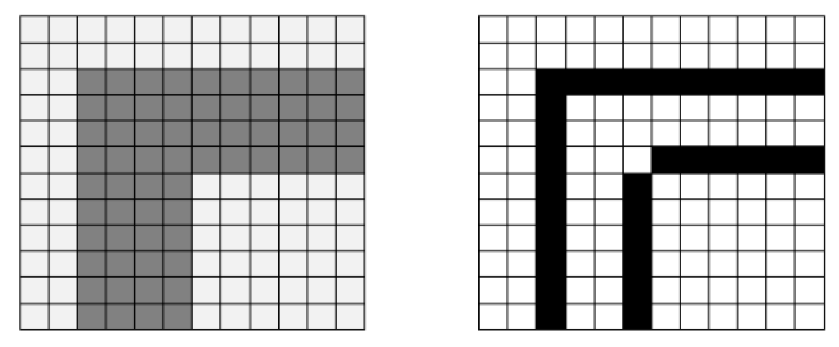
Let us consider the example in Figure 1. It contains a fragment of a rectangle border in dark gray (four pixels wide), surrounded by background in light gray, with a difference of more than 80 gray levels between dark and light gray. The leftmost dark pixels are identified as border pixels because they have adjacent light pixels on the left. This is the same for the uppermost dark pixels, and also for the pixels belonging to the inner border. On the contrary, those dark pixels inside the dark gray area are not identified as border pixels because they do not have light adjacent pixels, that is, a dark line that is wide enough (more than two pixels wide) can produce more than one line of border pixels. We will observe what happens with the “inner borders” later in Section 4.3.

Our work presents a novel approach, with respect to the traditional way, of identifying thresholds and borders, which are not identified in two separate steps (see Section 4.2), but simultaneously in a single processing of the image in order to improve efficiency. Therefore, we do not use a fixed threshold for the whole image, but a dynamic comparison depending on the environment of each pixel. After analyzing the gray histograms in the set of images, a heuristic value of 80 levels was chosen as a good discriminator; adjacent pixels with a difference less than 80 belong to the same area, otherwise, the darker pixel is identified as a line pixel.

4.2. Vertical and Horizontal Segment Identification

The next step is the identification of vertical and horizontal segments that are candidates to be either edges of UML shapes (rectangles) or else relationships between shapes, such as associations or generalizations (remember that we disregard oblique lines for the sake of computational efficiency). Here, we consider only the pixels that have passed the ‘line pixel’ detection filter in the previous step. As mentioned, the detection of line pixels and the identification of segments is actually performed in a single pass on the image to improve efficiency, even if we explain them as two consecutive steps for clarity.

The method consists of scanning the image pixel-by-pixel, downwards and rightwards. When a line pixel is found, the scanning continues first downwards to check whether it belongs to a vertical segment, and then rightwards to check for a horizontal segment. The scanning of a segment stops when it reaches the limits of the image or when more than five consecutive background pixels are found, that is, gaps up to five pixels (a heuristic value) are allowed in order to identify dashed lines and small defects in continuous lines. When an end-pixel is found to belong simultaneously to a vertical and a horizontal segment (with either ‘L’ or ‘T’ connection), then the connection between both segments is identified. Two segment ends that are close enough (less than five pixels apart, heuristic value) are considered as connected, too, in order to avoid false negatives in images with defects and other special cases (see the two inner segments in Figure 1).

Moreover, each segment is stored with the following attributes that will be useful for later processing:

• Unique sequential ID within the image. The comparison of identifiers of two segments provides information about their relative position within the image. For two vertical segments, the one with lower ID must be to the left of the other, or above. For two horizontal segments, the one with lower ID must be above, or to the left of the other.
• Position. Cartesian coordinates of the two ends of the segment. The length and orientation (vertical/horizontal) are derived attributes.
• Density. It is the ratio between the number of line pixels and the total number of pixels. A density of pixels lower than 80% tells the segment is discontinuous.
• Connected segments. When one of the two end pixels of a segment simultaneously belongs to another segment, then those two segments are connected. This does not include crossing segments, but it does include ‘T’ connections (see Figure 6 at the end of this section).

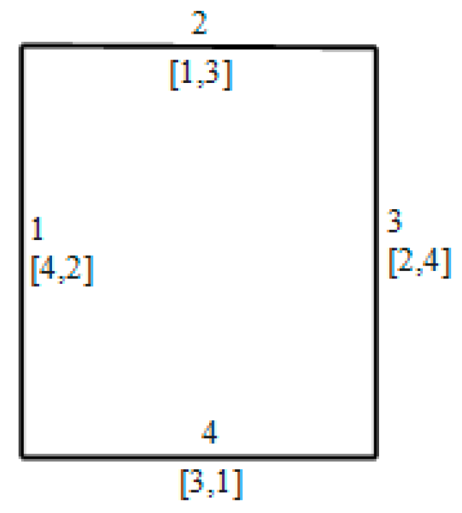
Figure 2 illustrates four segments that form a rectangle. Since the scanning of pixels is first undertaken downwards and then rightwards, the first segment identified is the left one, then the upper one, then the right one, then the lower one; IDs are assigned accordingly.

4.3. Rectangle Identification

Rectangles are used to represent classes and objects in UML static diagrams, in addition to being part of other more complex shapes such as packages, components and so on. The identification of rectangles is achieved using the vertical and horizontal segments identified according to the previous subsection. The objective is to find four cyclically connected segments whose identifiers go in ascending order (possibly with gaps among them). This last restriction is aimed at obtaining a unique representation of each rectangle as a sequence of its edges, starting with a vertical one. In addition, it is required that the segments are not discontinuous and have a minimum length of 10 pixels (another heuristic value; shorter segments usually are false positives).

A programmed automaton Ap = (Q, I, O, M, δ, q₀) [32,33] is used to recognize those sequences of segments that satisfy the mentioned restrictions, where:

Q 

The set of states.

I 

Input, the sequence of vertical and horizontal segments detected.

O 

Output, the sequence of vertical and horizontal segments forming a rectangle.

M 

Adjacency lists (segment connections) and other segment attributes.

δ 

Q × I × Π → Q × O: transition function.

Π 

A_I ∪ A_M → {TRUE, FALSE}: transition predicate.

A_I 

Set of attributes of I.

A_M 

Set of attributes of M.

q₀ 

∈ Q initial state.

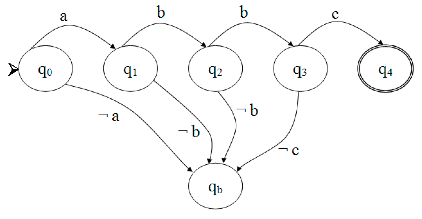
Figure 3 represents the programmed automaton, where q_i is the state where i consecutive segments are recognized as potential edges of a rectangle, q_b is the break state (i.e., the sequence of segments does not complete a rectangle) and Boolean expressions a, b and c are computed on the successive input segments as follows:

a

= currentSegment.continuous

• AND (currentSegment.length ≥ 10)
• If current segment is continuous and long enough,
• then jump to q₁, else q_b.
• Left vertical edge.

b

= a

• AND (previousSegment.id < currentSegment.id)
• AND currentSegment.connected(previousSegment)
• If current segment is continuous, long and connected to the previous one,
• then q₂ (or q₃) else q_b.
• Upper horizontal edge and right vertical edge.

c

= b

• AND currentSegment.connected(firstSegment)
• If current segment is continuous, long, connected to the previous one, and to the first one,
• then q₄ else q_b.
• Lower horizontal edge, completing the four required edges to form a rectangle.

Figure 4 illustrates the process of rectangle recognition with the defined automaton, with an example. In state q₁, the automaton found a continuous vertical segment. In state q₂, the automaton found a continuous horizontal segment, connected to the first segment and with a greater ID. In state q₃, the automaton found a continuous vertical segment, connected to the second segment and with a greater ID. In state q₄, the automaton found a continuous horizontal segment, connected to the third segment and with a greater ID, and connected to the first segment.

Once all rectangles present in the image are recognized, we distinguish primary and secondary rectangles. Primary rectangles are not contained by other rectangles; secondary rectangles are contained within other (primary or secondary) rectangles, i.e., their four vertices are enclosed within the limits of another rectangle.

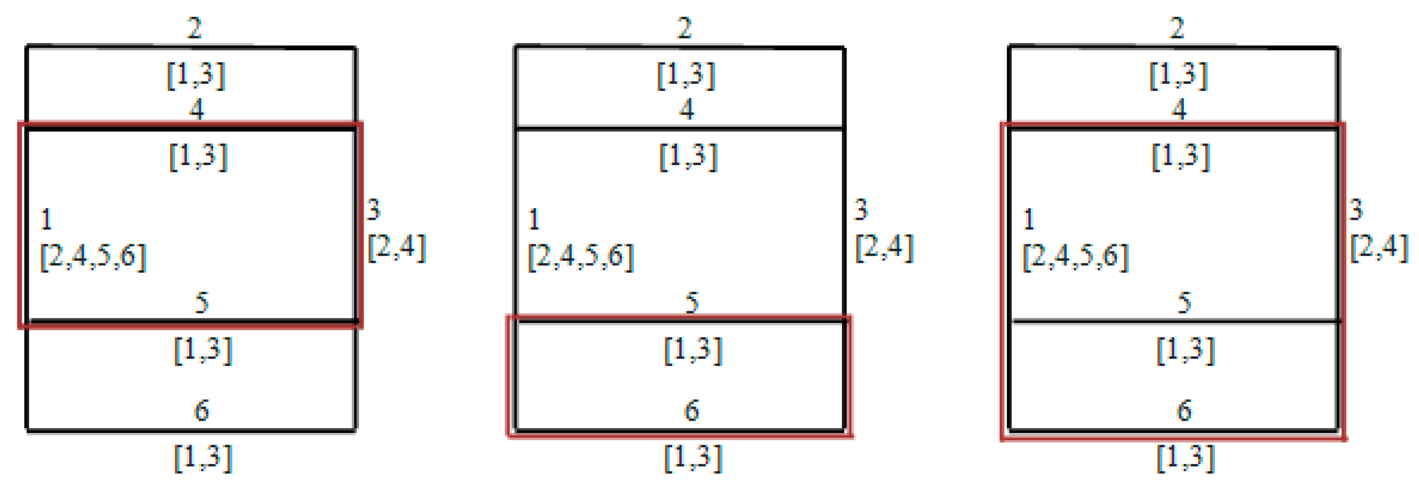
This process is efficient thanks to the way segments are assigned their IDs. A typical UML class symbol contains three compartments (see Figure 5); however, the combination of segments can produce up to five different contained rectangles. The rule, used to assign segment IDs, automatically discards three of them without the need of checking containment (see Figure 6), so that the distinction between primary and secondary rectangles is more efficient.

Figure 6 shows three contained rectangles that are automatically discarded by the automaton, since their third edge belongs to a segment whose ID (No. 3) is lower than its preceding upper segment (respectively No. 4, 5 and 4). This simplification in the number of cases of included rectangles to be examined improves the efficiency in the identification of primary rectangles. This also solves the problem of spurious or duplicate rectangles that can result of the “inner borders” problem (examined in Section 4.1) in a reduced computational time.

Summing up, the feature extraction stage described in this section assumes the following heuristic values for the parameters:

• Gray difference between line pixels and surrounding pixels: 80 gray levels. Adjacent pixels with a difference less than 80 belong to the same area, otherwise the darker pixel is identified as a line pixel. In other words, a pixel belongs to a line if it has a horizontally or vertically adjacent pixel with a gray intensity at least 80 levels above, in a scale from 0 (black) to 255 (white).
• Gaps in dashed lines: five pixels. Gaps up to five pixels are allowed in order to identify dashed lines and small defects in continuous lines. Equally, when two segment ends are less than five pixels apart, then these two segments are considered as connected, in order to avoid false negatives in images with defects and other special cases.
• Density of line pixels in continuous segments: at least 80%. A density of pixels lower than 80% tells the segment is discontinuous. Rectangles identified by the automaton must have all segments continuous.
• Minimum length for rectangle segments: 10 pixels. In addition to being continuous, it is required by the automaton that the segments belonging to a rectangle have a minimum length of 10 pixels.
• Minimum length for vertical/horizontal segments: 30 pixels. This parameter is not used in the feature extraction stage, but in the learning algorithm (see Section 6), which distinguishes short and long segments present in the image.

These values are grounded in previous research about image processing in traffic signals [31]. We considered that they are sufficiently well established and that is why we did not include them within the learning approach. On the other hand, allowing the algorithm to learn these values together with the classification rules would make the learning process computationally inefficient. We do not think that the robustness of the system is compromised, as our experimental results show.

5. Classification Functions in the Hyperspace of Graphical Characteristics

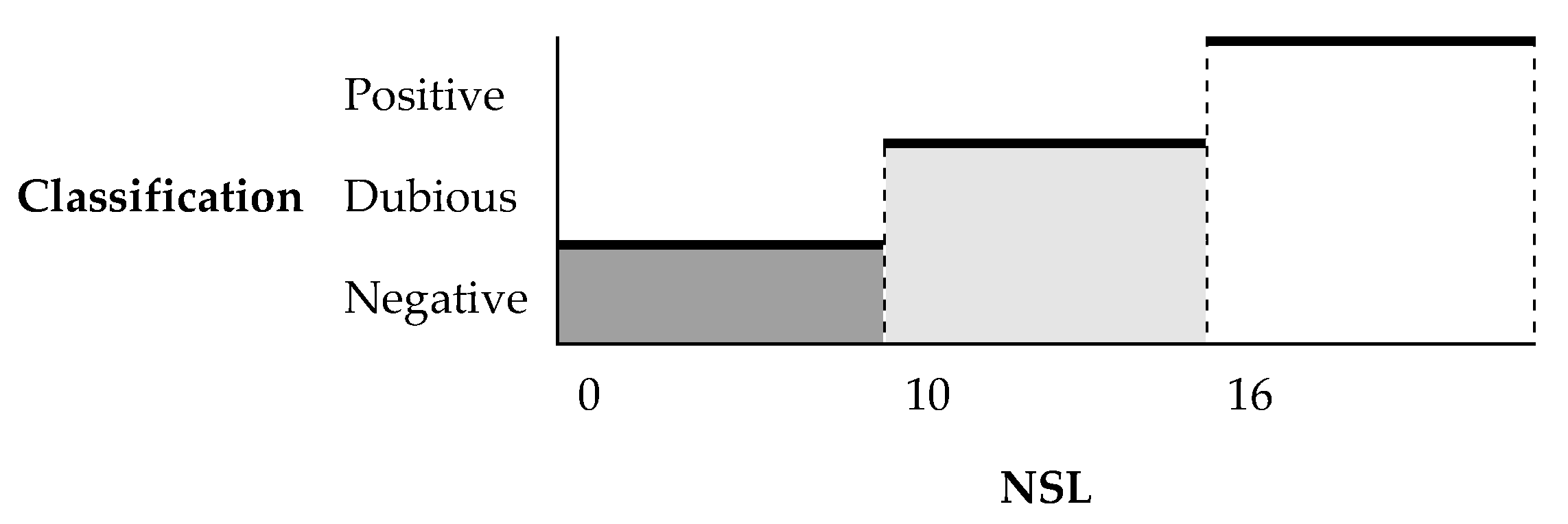
Suppose we classify images by their graphical characteristics based on a single variable or metric, for example the number straight lines (NSL) present in the image. We can then formulate a simple rule to transform the metric into a classification, such as “if NSL ≤ 10 then Negative, else Positive”. The rule can be easily refined to account for more classifications, using more intervals in the value of the metric, such as “if NSL ≤ 10 then Negative, else if NSL ≤ 16 then Dubious, else Positive” (see Figure 7). For simplicity, since the argument is easily generalizable to any number of classifications, we will assume in the rest of the paper that the number of levels is only two: Negative or Positive.

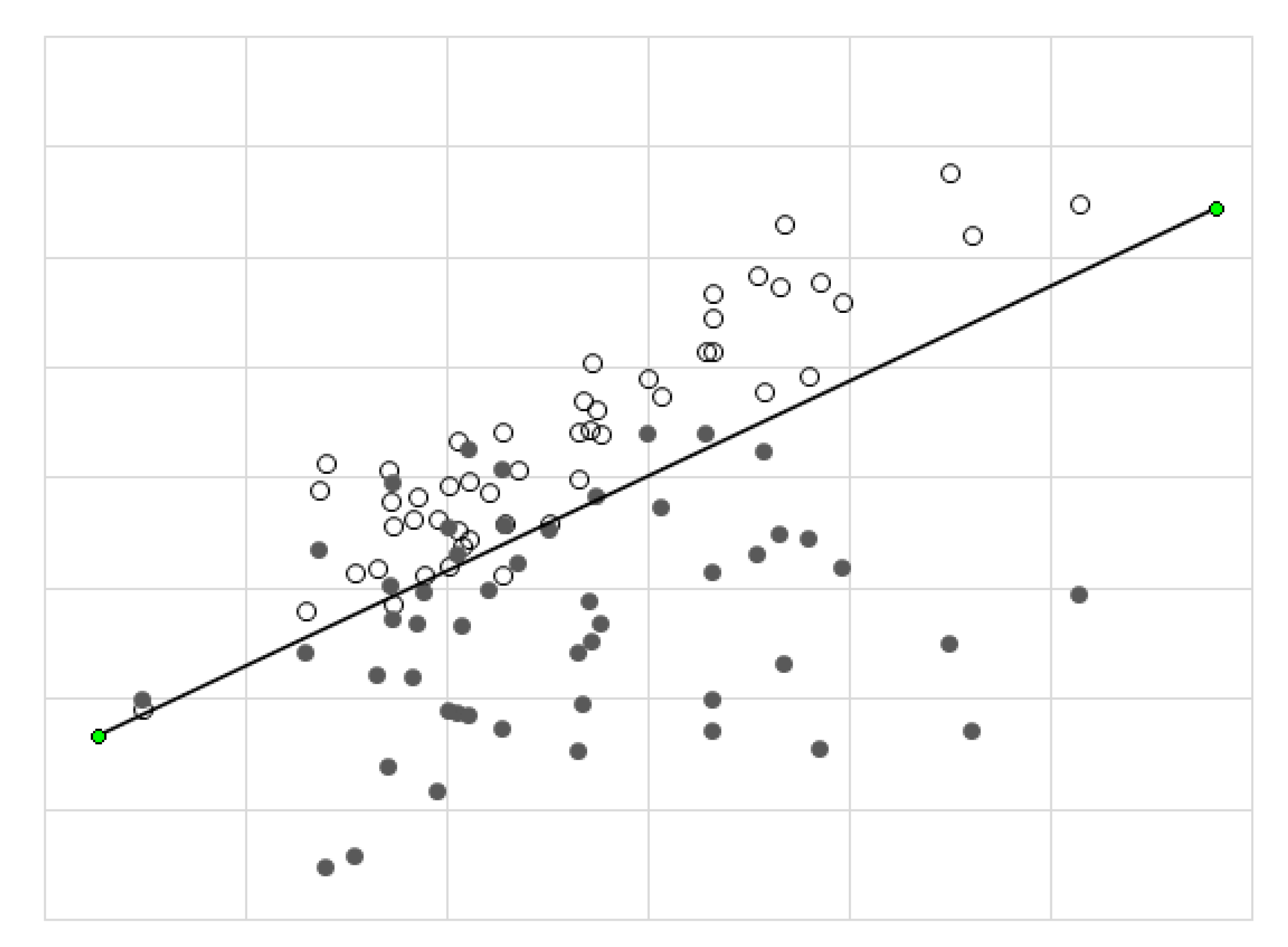
Now, suppose we want to combine two different metrics to assign a classification, such as number of rectangles (NR) and number of gray tones (NG). We can represent both variables on the X–Y plane, where each point is an image and the point color is the classification. The simplest way to classify the cloud of points is by a linear combination of the variables, i.e., the traditional method of weighted average of metrics: “if (a*NR + b*NG) ≤ L, then Negative, else Positive”, where a, b and L are convenient values. When the cloud of points is naturally split into two regions separated by a straight line, the values of a, b and L can be easily obtained with simple mathematical methods (see Figure 8). The method generalizes to any number of dimensions (metrics) that define a hyperspace of graphical characteristics split in two regions by a hyperplane.

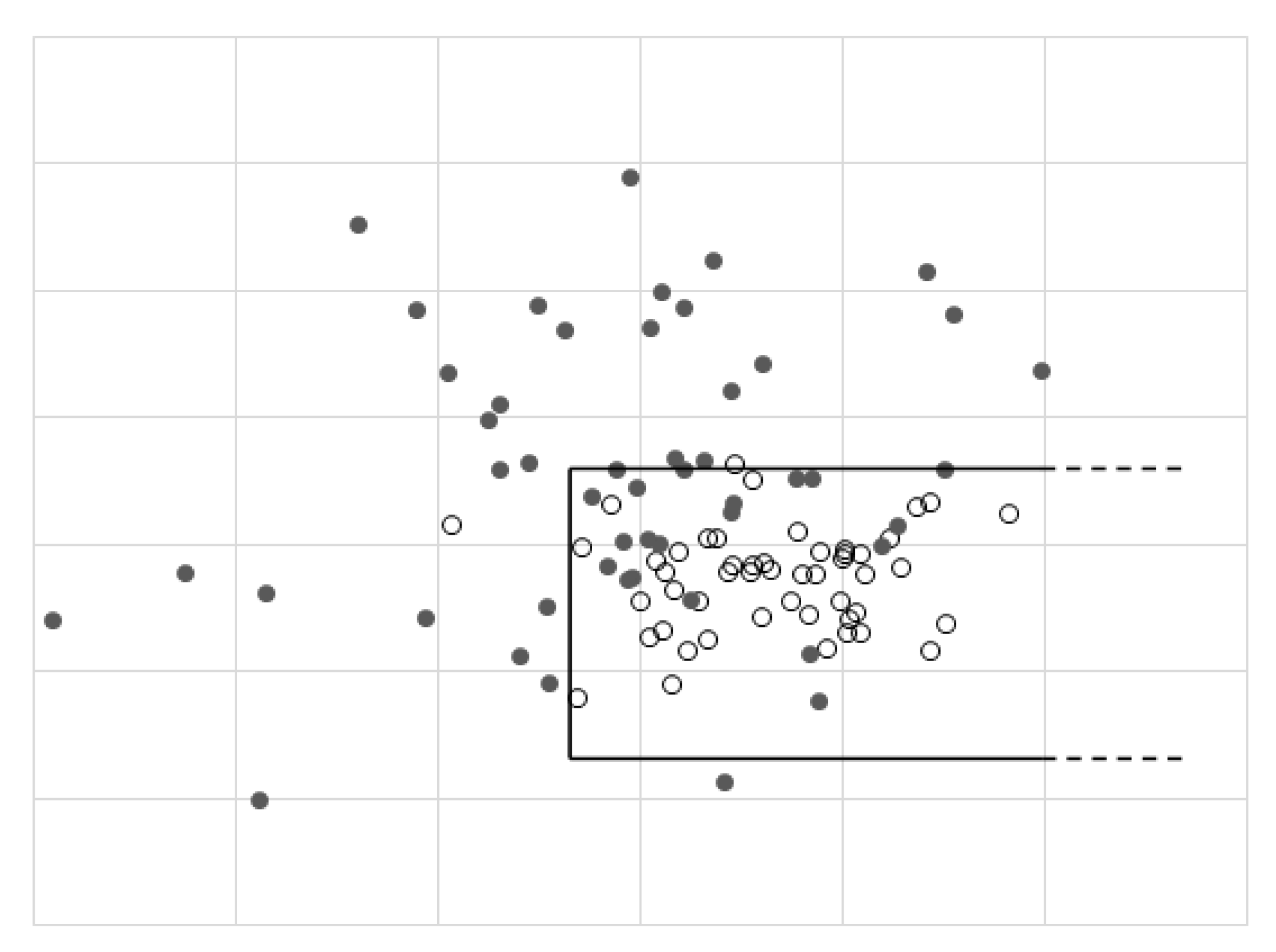
However, this simplicity is not usually found when the variables present a more complex relationship with the classification, which can be very difficult to estimate a priori (see Figure 9). In these situations, a more convenient yet simple way to combine the metrics is by means of a rectangular region: the classification is Positive inside the region, otherwise it is Negative (or vice versa). Note that the region could be open in one or more sides: “if NR between [10, –] and NG between [2, 40] then Positive, else Negative”. The method is also rather simple and generalizes to hyper-rectangular regions in the hyperspace of graphical characteristics.

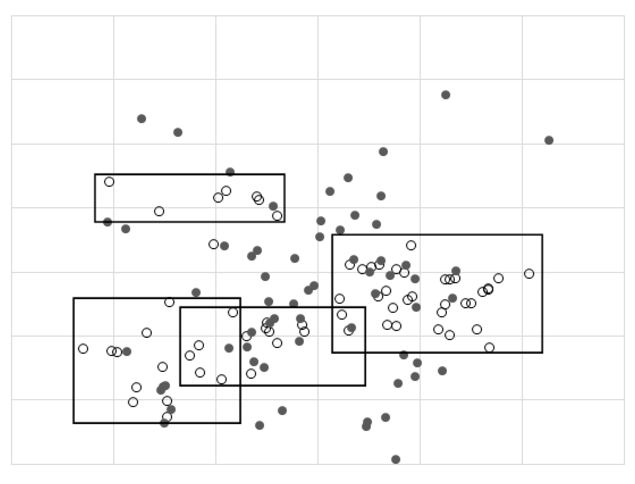
The most common case in the combination of metrics, however, is not so simple, and the cloud of points is not easily discriminated by a single (hyper-) rectangle. In these situations, we can still generalize the procedure to a combination of regions that can be better adjusted to the cloud of points (see Figure 10), such as: “if NR between [10, 20] and NG between [2, 40] then Positive, else if NR between [20, –] and NG between [2, 15] then Positive, else Negative”. Note, the regions could be overlapping (requiring that they do not overlap could produce a worse adjustment of the rule, or a more complex rule with more rectangles).

Summing up, the discrimination of regions by means of hyperplanes (Figure 8) is generally very inadequate, and the use of simple rectangular regions (Figure 9) is still insufficient. Instead, a combination of rectangular regions (Figure 10) is a versatile method when the different metrics employed present complex relationships manifested in the clustering of points. The higher the number of regions, the better the adjustment of the discriminating rule to the dataset (avoiding of course an excessive number of regions, which would compromise generality). However, computing the concrete intervals for each metric becomes a difficult problem. This is where machine learning techniques prove particularly useful to generate the rules.

6. Selection of Graphical Characteristics and Rule Induction by Machine Learning Techniques

The discrimination of images representing UML static diagrams is achieved in this project by an automatic classifier that uses data mining techniques of supervised learning. Machine learning techniques are mechanisms used to obtain patterns through the analysis of data. This is a well-known subfield of computer science that evolved from the study of pattern recognition and computational learning theory in artificial intelligence, therefore we provide only a brief explanation. Machine learning explores the construction and study of algorithms that can learn from data, by building a model from example inputs in order to make data-driven predictions or decisions, rather than following strictly static program instructions [34]. On the other hand, Search-Based Software Engineering is an approach in which search-based optimization is applied to software engineering [35]. Machine learning, then, is one of the techniques that can be used to perform search-based software engineering.

Machine learning techniques can be supervised or unsupervised [36,37]:

• Supervised learning: the algorithm is presented with example inputs and their desired outputs, and the goal is to learn a general function that maps inputs to outputs.
• Unsupervised learning: the inputs to the learning algorithm are given no output labels, leaving the algorithm on its own to find structure in the inputs.

More specifically, supervised learning is the task of inferring a function from labeled training data, where each input is described by a vector of common attributes (see Figure 11).

The training data consist of a set of training examples, each example consisting of an input object (in our case, the vector of graphical characteristics obtained from an image downloaded from the web) and a desired output value (in our case, the manual classification as a UML static diagram, or not, judged by the expert). The input attributes we have used in this project are:

(1)

Number of gray tones.

(2)

Number of color hues.

(3)

Number of vertical/horizontal segments.

(4)

Number of vertical/horizontal segments at least 30 pixels long.

(5)

Number of horizontal segments at least 30 pixels long.

(6)

Number of vertical segments at least 30 pixels long.

(7)

Number of rectangles.

(8)

Number of main rectangles (not included in other rectangles).

Note, we use the number of vertical/horizontal segments in four different ways, in order to increase their discriminatory power.

A supervised learning algorithm analyzes the training data and infers a generalized function, which can be used for classifying new inputs. The effectiveness of the automatic classifier obtained is then measured against the testing set, which was previously segregated from the initial data, so that training and testing are performed with different datasets.

In terms of search-based software engineering, the optimization problem consists in finding a function of the graphical characteristics (a piecewise function defined by a set of rules), such that it minimizes the distance with the experts’ classification over the set of all images. This can receive the following mathematical formulation:

• Let P be a set of images, or pictures,$\mathrm{P}=\left\{{\mathrm{p}}_1,\dots ,{\mathrm{p}}_{\mathrm{n}}\right\}$.
• Let C be the classifications over the set of pictures, $\mathrm{C}=\left\{{\mathrm{c}}_1,\dots ,{\mathrm{c}}_{\mathrm{n}}\right\}$ such that ${\mathrm{c}}_{\mathrm{i}}\in \left\{0,1\right\}$ is the class provided by the experts to picture ${\mathrm{p}}_{\mathrm{i}}$, where 0 represents “not a static diagram” and 1 represents “a static diagram”.
• Let G be a set of graphical characteristics obtained from pictures,$\mathrm{G}=\left\{{\mathrm{g}}_1,\dots ,{\mathrm{g}}_{\mathrm{k}}\right\}$, such that ${\mathrm{g}}_{\mathrm{j}}:\mathrm{P}\to ℝ\left(1\le \mathrm{j}\le \mathrm{k}\right)$.

Goal:

Find a function $f:{ℝ}^k\to \left\{0,1\right\}$ such that it minimizes

$${\displaystyle \sum }_{i=1}^n|f\left(g_1\left(p_i\right),\dots ,g_k\left(p_i\right)\right)-c_i|$$

There are several kinds of machine learning techniques. Among them, neural networks are the most widely used today as a de facto standard tool in computer vision. However, as is well known, one of the main drawbacks of neural networks is that they provide black boxes whose only justification for the functions obtained is the effectiveness they reach. Therefore, we selected a different machine learning technique, namely rule induction, because it provides a human-readable decision algorithm that improves the explainability and modifiability of the classification model obtained by a good amount. Even if the neural networks approach could reach better effectiveness, it would be at the price of losing all expressiveness and interpretability of the classification model. In any case, we provide a comparison of experimental results obtained with both approaches in the next section.

Rule induction (or rule inference) techniques are a kind of supervised learning that process input training data and produce a set of IF-THEN rules used to classify the new examples [38,39]. Two main strategies are commonly used:

• Produce a decision tree and then extract its rules.
• Generate the rules covering all the examples in a given class, exclude the covered examples and proceed with the next given class, until all classes are covered.

The first strategy is implemented in the C4.5 system [40], which extends the previous ID3 [41]. Other algorithms such as PRISM [42] are based only on covering, whilst PART [43] combines both strategies. These strategies present the following advantages to minimize the impact of unintentional errors in the expert’s classification of the images used as training examples:

• Robustness against noise due to errors, omissions or insufficient data.
• Identification of irrelevant attributes.
• Detection of absent attributes or knowledge gaps.
• Extraction of expressive and easy to understand rules.
• Possibility to interpret or modify the produced rules with aid of expert knowledge, or even to incorporate new rules inferred by the experts themselves [44].

In order to improve the effectiveness of the individual classifiers obtained by means of rule induction, ensemble methods construct a set of classifiers and then classify new instances by taking a vote of their decisions (it can be a weighted vote, the mode of the votes, etc.) [45]. The technique has two main variants:

• Homogeneous classifiers are generated with the same learning algorithm [46]. The main methods are Bagging [47] and Boosting [48].
• Heterogeneous classifiers, instead, are generated with different learning algorithms. The most used method is Stacking (Stacked Generalization) [49].

We finally chose the Bagging method of homogeneous classifiers on the basis of the rule induction PART algorithm [43] to perform the experiments and obtain the classifiers. We explain the experiments in detail in the next section.

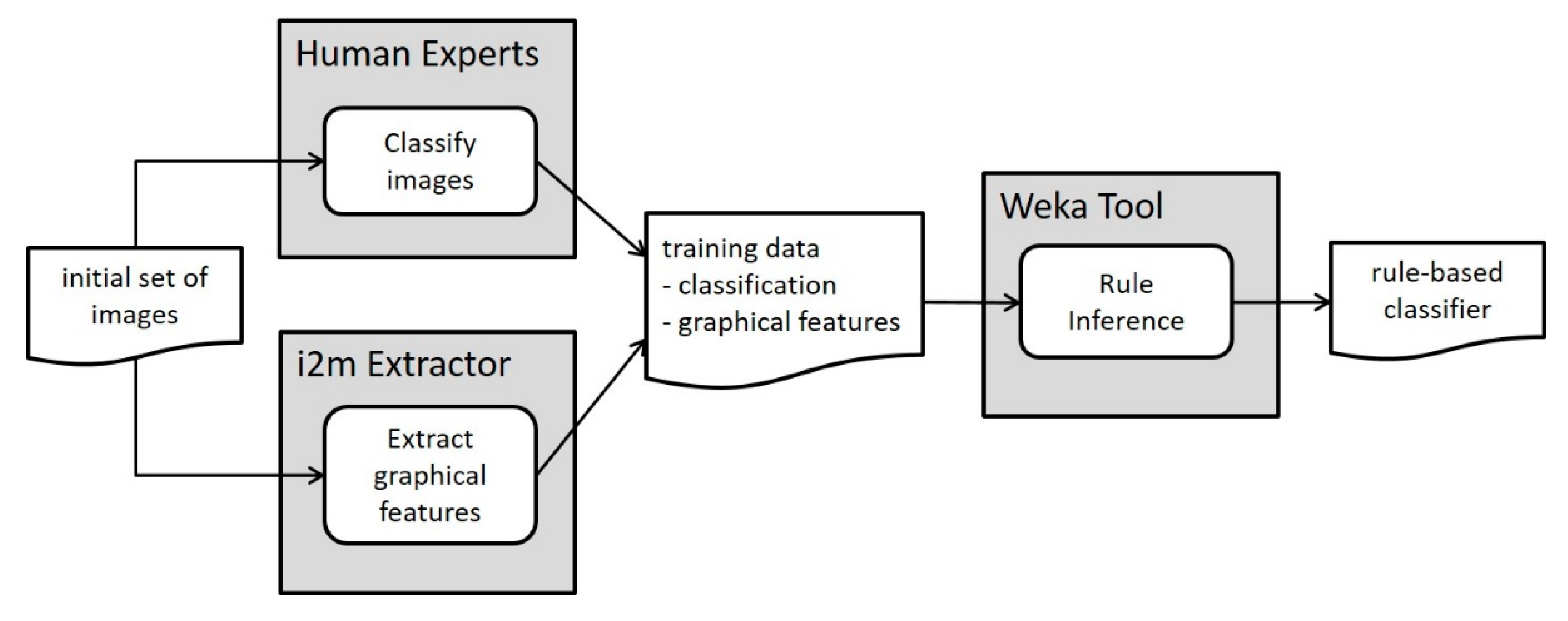
The whole process consists of two main stages: rule inference and rule application. The inference stage can be summarized in the following steps (see Figure 12):

• Obtain the initial set of images downloaded from the web.
• Classify the images according to the criteria explained in our previous conference paper [9] (done by human experts).
• Extract the graphical features described in Section 4 (number of gray and color tones, and number of straight lines and rectangles) (done by the i2m tool extractor).
• Build the training and testing data for the supervised machine learning algorithm, combining the two previous outputs: each image is represented as a vector of graphical features and human-assigned classification.
• Launch the rule inference learning algorithm (in our case, run in the Weka tool) to obtain as output the automatic classifier, i.e., the function made of rules that classifies images as UML static diagrams or otherwise, thus emulating the human experts.

Once we have built a validated rule-based classifier, we implement the rules in our tool (see Section 8) and use it in the application stage to automatically classify new images as the emulated human experts would do (see Figure 13):

7. Experiments and Results Obtained

As explained, we applied the rule induction PART algorithm combined with the Bagging approach of homogeneous classifiers. The experiments were implemented in the popular Weka suite [50], keeping its standard default parameter configuration. We used the set of 18,899 images downloaded from the web as training examples, manually classified by the experts as explained in our previous conference paper [9]. From this initial dataset, a combination of rules was extracted with the PART algorithm that can be extrapolated to classify new images.

Some examples of the individual rules automatically obtained are:

IF (number-of-primary-rectangles ≤ 0) AND (number-of-segments ≤ 11)

THEN Negative (it is not a diagram)

This rule classified 9,445 of our 18,899 examples as non-diagrams,

with 55 false negatives (0.6%).

IF (number-of-primary-rectangles > 2) AND (number-of-hues ≤ 6)

THEN Positive (it is a diagram)

This rule classified 176 examples out of 18,899 as diagrams,

with 7 false positives (4%).

As explained, the algorithm provides not only individual rules, but also a function that combines the rules and maximizes the overall results. We performed 10 experiments with the available dataset. In each experiment we used the 794 positive instances (manually classified as UML static diagrams, see our previous conference paper [9]) together with other 794 negative instances (other non-UML static diagrams and non-diagrammatic pictures), randomly chosen, without replacement, from the total set of negative instances. We performed the usual 10-fold cross validation [51], obtaining the classifiers shown in

Table 3. Summary of the results of the classifiers obtained with the 10 experiments: precision, recall and percentage of agreement in classifying images as UML static diagrams.

Experiment	Precision for Positives	Recall for Positives	Precision for Negatives	Recall for Negatives	Percentage of Agreement
1	0.956	0.928	0.930	0.957	94.3%
2	0.950	0.933	0.934	0.951	94.2%
3	0.945	0.943	0.943	0.945	94.4%
4	0.965	0.936	0.938	0.966	95.1%
5	0.963	0.942	0.943	0.963	95.3%
6	0.956	0.931	0.933	0.957	94.4%
7	0.936	0.923	0.924	0.937	93.0%
8	0.955	0.940	0.941	0.956	94.8%
9	0.952	0.923	0.925	0.953	93.8%
10	0.953	0.929	0.931	0.955	94.2%
Average	0.953	0.933	0.934	0.954	94.4%

.

For the purpose of comparison, we repeated the experiments with the neural networks approach, i.e., using the same Bagging method of homogeneous classifiers, this time on a multilayer perceptron (the Weka tool has default options to automatically build the network). The results are shown in

Table 4. Results of the classifiers obtained with a multilayer perceptron.

Experiment	Precision for Positives	Recall for Positives	Precision for Negatives	Recall for Negatives	Percentage of Agreement
1	0.953	0.927	0.929	0.955	94.1%
2	0.956	0.927	0.929	0.957	94.2%
3	0.960	0.941	0.942	0.961	95.1%
4	0.961	0.923	0.926	0.962	94.3%
5	0.967	0.931	0.933	0.969	95.0%
6	0.965	0.928	0.931	0.966	94.7%
7	0.937	0.924	0.925	0.938	93.1%
8	0.962	0.935	0.936	0.963	94.9%
9	0.951	0.928	0.930	0.952	94.0%
10	0.960	0.932	0.934	0.961	94.6%
Average	0.957	0.930	0.932	0.958	94.4%

. As can be observed, there is no statistically significant difference between both approaches, that is, both methods are completely equivalent regarding the effectiveness of the classification.

8. The i2m Classification Tool

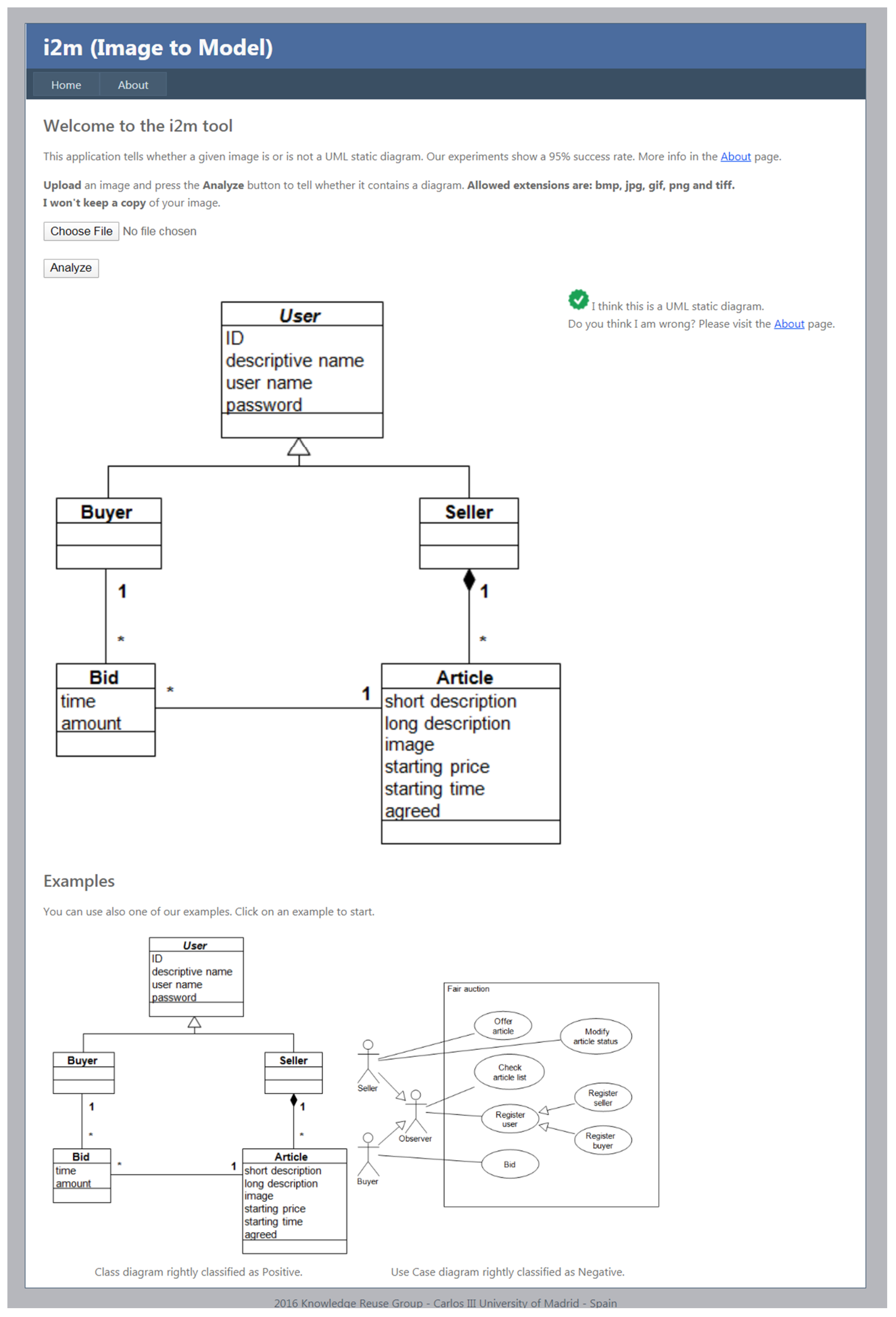
We developed the experimental i2m (image-to-model) tool according to the principles exposed in this research (see Figure 14). The current version of the tool (i2m v1.0, image-to-model tool: http://i2m.kr.inf.uc3m.es) accepts a bitmap file (in different formats) as the input and deduces whether the image corresponds to a UML static diagram in less than 1 s. More precisely, according to the data of four years working, the average time to extract the graphical features is 715 milliseconds, whilst the time to automatically classify the image is only a few milliseconds, which is negligible by comparison. The tool is freely accessible on the web.

9. Conclusions and Future Work

Even though the usage of machine learning techniques for the emulation of human judgment have been numerous in widely differing contexts, there are scarce references in literature, to our knowledge, that describe their application for image classification as diagrams in the field of software engineering, which is why we consider our research to be a manifestation of a high degree of novelty.

We developed a method and a tool (i2m, image-to-model v1.0, http://i2m.kr.inf.uc3m.es) to classify web images in different formats (BMP, GIF, JPEG, PNG and TIFF) as UML static diagrams, without requiring the images to be explicitly or implicitly tagged as UML diagrams. The tool uses a combination of rules acquired through machine learning techniques on a dataset of nearly 19,000 instances; the rules consider graphical characteristics of images, such as grayscale histogram, color histogram, number of straight lines and rectangles and so on.

Table 5. Comparison of the results of our method with those of related work.

Research	Number of Attributes	Number of Images	Processing Time/Img.	Accuracy
Karasneh and Chaudron [22] (not a machine learning approach)	N/A	200	N/A	89.0%
Hjaltason and Samúelsson [24]	23	1,300	10 s	91.2%
Ho-Quang et al. [25]	19	1,300	5.84 s	90.7%–93.2%
Hebig et al., 2016 [26] (same classifier as [25])	19	19,506	4.89 s	N/A
This research	8	18,899	0.68 s	94.4%

repeats the information in Table 1 and compares it with our own results. We can observe that our method produces better results in all the items considered:

• It uses less than half of the graphical attributes to classify diagrams.
• The training dataset is nearly 15 times bigger (remember, [26] does not use a new dataset to train their classifier, but only to validate the one they borrow from [25]).
• Accuracy (the percentage of agreement with the manual classification) is higher.
• Very notably, the time required to process each image and extract its graphical features is seven times lower, due to the fact that we use ad-hoc instead of standard computer vision techniques and libraries.

In

Table 6. Comparison of the results of our method with those of Ho-Quang et al. [25].

Algorithm	Precision for Positives	Recall for Positives (Sensitivity)	Precision for Negatives	Recall for Negatives (Specificity)	Accuracy
Support Vector Machine	0.894	0.924	0.921	0.890	90.7%
Random Forest	0.909	0.959	0.957	0.904	93.2%
J48 Decision Tree	0.903	0.925	0.923	0.901	91.3%
Logistic Regression	0.913	0.902	0.903	0.914	90.8%
REP-Tree	0.903	0.920	0.918	0.901	91.1%
Decision Table	0.897	0.919	0.917	0.895	90.7%
This research	0.953	0.933	0.934	0.954	94.4%

we compare our average performance with the results of the six algorithms of Ho-Quang et al. already shown in Table 2. We can observe again that our results are generally better in the five metrics exposed. If we compare our results with their best algorithm from the points of view of accuracy or sensitivity, Random Forest, we are still around 5% better in two items (precision for positives, recall for negatives), even if they are 2% better in other two items (recall for positives, precision for negatives). Considered as a single measure, our accuracy is 1% better than theirs, which is not too significant, but nevertheless better. Compared with their favorite algorithm, Logistic Regression (because its highest specificity), we are better in the five metrics, including specificity.

Moreover, we compared the effectiveness achieved by our machine learning approach (rule induction) with a neural network approach (multilayer perceptron) used as a baseline, finding that there is no statistically significant difference (see Table 4 in Section 7). In other words, our approach improves explainability and processing time without losing effectiveness.

With nearly 95% accuracy (percentage of agreement with manually classified instances), this tool is useful for the improvement of the effectiveness of common web image search engines like Google Images. The tool is useful also for searching private repositories in an organization, when metadata are not available.

This research project is focused on the development of a UML-oriented information retrieval tool. However, once the technology has been fully developed, it could easily be expanded to be applied in different and promising domains, such as building plans, electrical circuitry and so on.

We plan to develop future versions of the tool that will implement the following features:

• Classify a set of images, instead of one-by-one images.
• Classify other kinds of diagrams (use case diagrams, state transition diagrams and so on).
• Desktop version with the capability to explore private repositories.
• Use the output of a generic search engine (such as Google) as an input to the tool, so that the tool is used to further filter the output of the generic search engine and improve its precision.
• Integrate the image classification tool in a specific UML-oriented search engine, including a web crawler that indexes UML diagrams, with the potential to improve not only precision, but also recall.
• Extract textual information from the diagram with the aid of OCR technologies. Combine with the previous feature to search the web for specific diagrams containing a given text.
• Interpret the diagram according to the UML metamodel, producing its output as a model in XMI format.
• Generate a graphical UML representation of the extracted model.

All these ongoing developments, each one with different degree of completion, form part of a larger UML-oriented information retrieval project.