The Influence of Main Design Parameters on the Overall Cost of a Gearbox

 ,
,  ,
,
Abstract
1. Introduction
2. Optimization Problem
2.1. Cost Analysis of Three-Stage Helical Gearbox
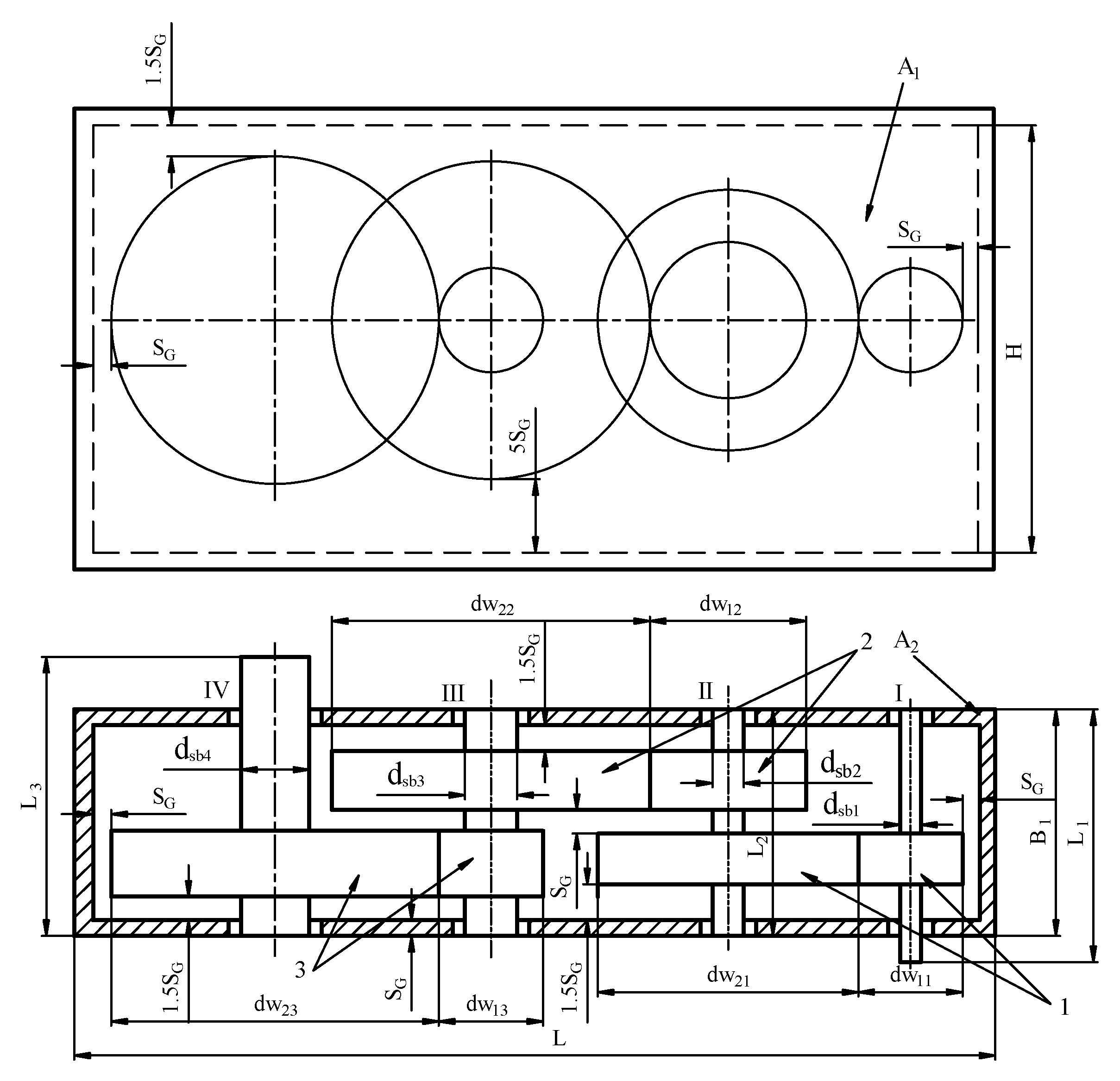
2.2. The Determination of Gearbox Housing Mass
2.3. Gear Mass Calculations
2.4. Shaft Mass Calculation
2.5. Determination of the Centre Distances of the Gear Stages
- –
- is the contacting load ratio for pitting resistance selected by 1.1 [12];
- –
- is the allowable contact stress of the i stage (MPa);
- –
- is the material coefficient; As the gear material is steel, = 43;
- –
- is the coefficient of wheel face width of the i stage;
- –
- is the torque on the drive shaft of the i stage (Nmm) determined by:
2.6. Optimization Problem
3. Experimental Work
4. Results and Discussions
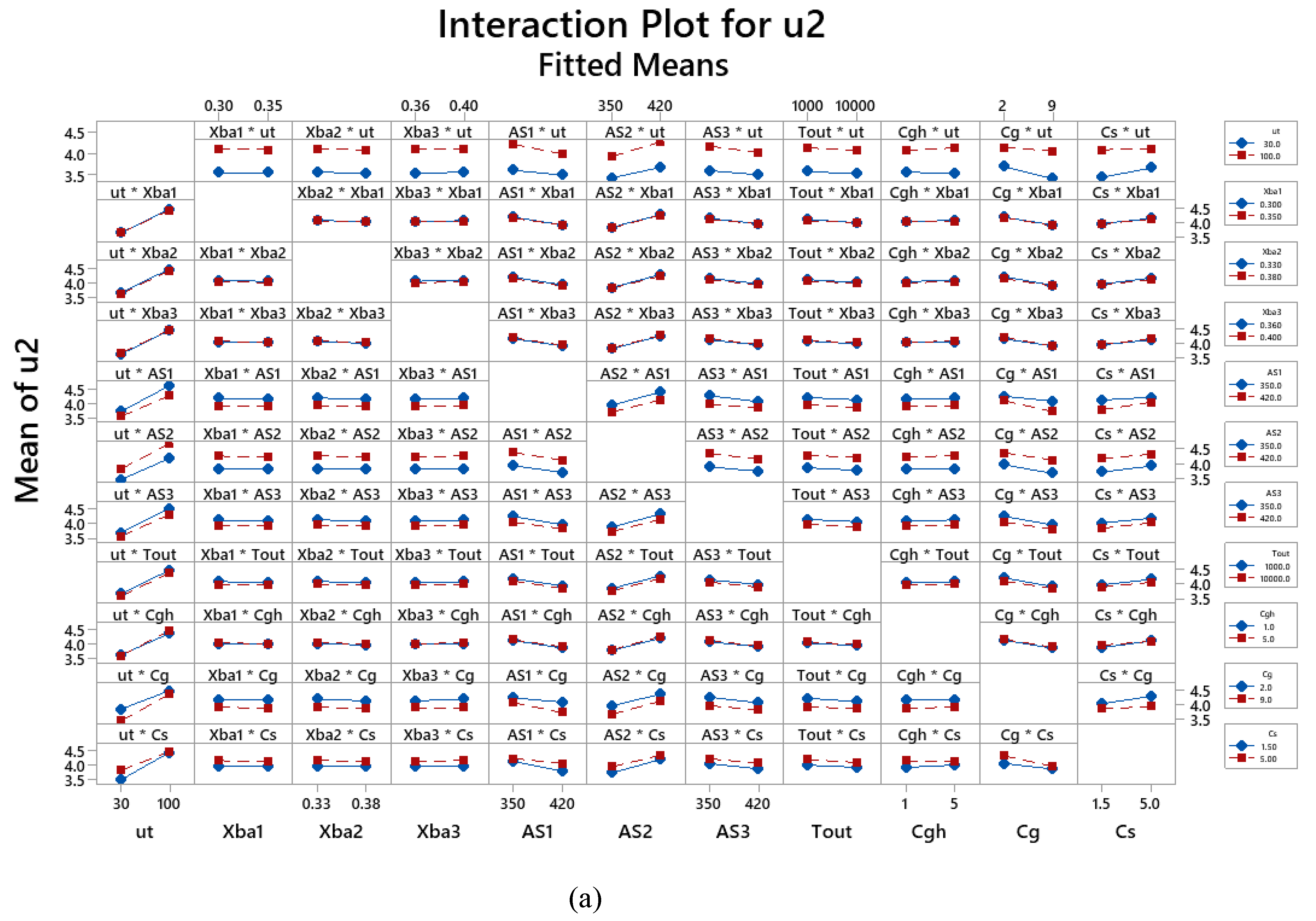
4.1. The Influence of Input Parameters and Their Interactions
4.2. Proposed Regression Model of the Response
− 0.00686 AS3 − 0.000058 Tout + 0.00397 Cgh + 0.1013 Cg + 0.1261 Cs − 0.000036 ut*AS1
+ 0.000030 ut*AS2 − 0.000014 ut*AS3 + 0.000405 ut*Cgh + 0.000587 ut*Cg − 0.001144 ut*Cs
+ 0.000131 Xba1*Tout − 0.327 Xba2*Cs − 0.2243 Xba3*Cg + 0.000012 AS1*AS3
− 0.000404 AS1*Cg + 0.000670 AS1*Cs + 0.000101 AS2*Cg − 0.000218 AS2*Cs
+ 0.000105 AS3*Cg + 0.000001 Tout*Cg − 0.00676 Cgh*Cs − 0.007003 Cg*Cs
+ 0.000197 Tout − 0.1537 Cgh − 0.079 Cg + 0.072 Cs − 0.000575 Xba1*Tout
+ 1.404 Xba1*Cs − 0.0737 Xba3*AS3 − 0.000053 AS1*AS3 + 0.000524 AS1*Cg
− 0.000528 AS3*Cg + 0.01440 Cgh*Cg − 0.03934 Cg*Cs
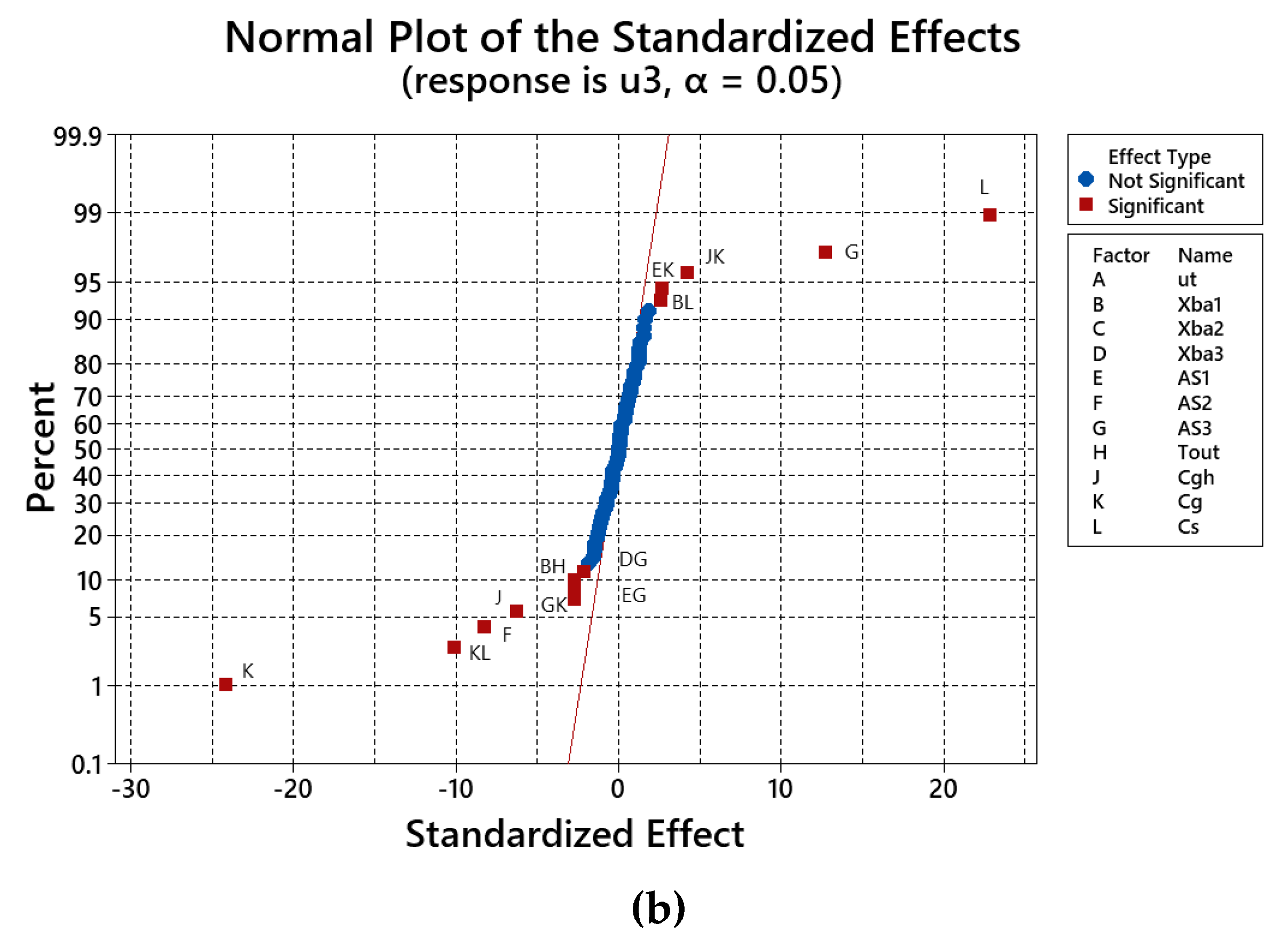
4.3. Analysis of Variance—ANOVA
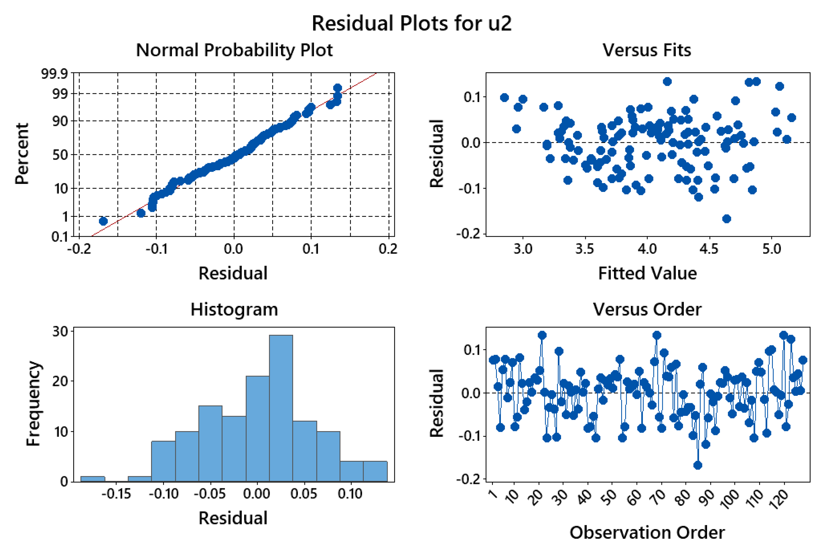
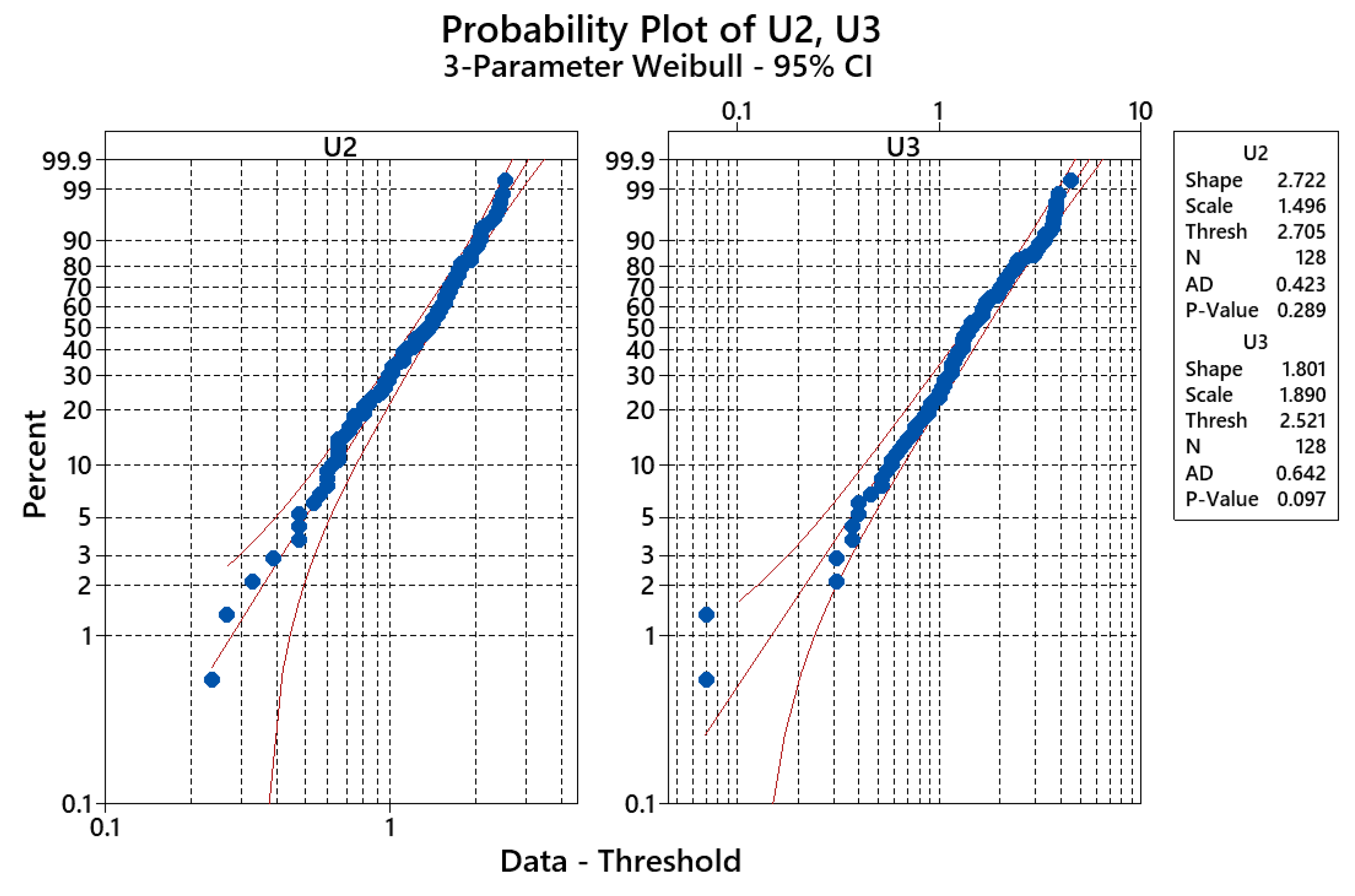
4.4. Validation of Proposed Model
5. Conclusions
- ✓
- The influence of input parameters and their interactions on response is different from those of response. The ANOVA results showed that the parameters of A, F, K, E, L, G, AK, AL, EK, AE, KL, H, EL, AF, AJ, and JL have significant influence on response (R-square value approaching 98%), while the corresponding to be the parameters of K, L, G, KL, F, and J in case of (R-square of 92%).
- ✓
- The parameters having insignificant influence were eliminated, inversely, the others that had strong influence would be considered for deeper experiments.
- ✓
- The proposed models of both and responses are highly consistent to experimental data. The reliability of the models is validated. It can be said that the proposed models can be applied to optimize the costs of gearbox.
Author Contributions
Funding
Acknowledgments
Conflicts of Interest
Appendix A
| Run Order | CenterPt | Blocks | ut | Xba1 | Xba2 | Xba3 | AS1 | AS2 | AS3 | Tout | Cgh | Cg | Cs | u2 | u3 |
| 1 | 1 | 1 | 30 | 0.35 | 0.38 | 0.4 | 350 | 420 | 350 | 1000 | 1 | 2 | 1.5 | 4.02 | 3.64 |
| 2 | 1 | 1 | 100 | 0.35 | 0.33 | 0.36 | 420 | 350 | 420 | 1000 | 5 | 2 | 1.5 | 4.08 | 4.24 |
| 3 | 1 | 1 | 100 | 0.3 | 0.33 | 0.4 | 420 | 350 | 350 | 1000 | 5 | 9 | 5 | 4.11 | 3.73 |
| 4 | 1 | 1 | 30 | 0.35 | 0.33 | 0.4 | 350 | 350 | 350 | 1000 | 5 | 2 | 1.5 | 3.63 | 3.58 |
| 5 | 1 | 1 | 100 | 0.3 | 0.33 | 0.36 | 350 | 420 | 350 | 1000 | 5 | 9 | 1.5 | 5.22 | 2.59 |
| 6 | 1 | 1 | 30 | 0.35 | 0.38 | 0.4 | 420 | 350 | 350 | 10000 | 5 | 9 | 1.5 | 3.03 | 3.28 |
| 7 | 1 | 1 | 100 | 0.3 | 0.33 | 0.4 | 420 | 420 | 420 | 10000 | 5 | 2 | 5 | 4.62 | 5.14 |
| 8 | 1 | 1 | 100 | 0.35 | 0.38 | 0.36 | 350 | 420 | 350 | 1000 | 5 | 2 | 1.5 | 5.07 | 3.25 |
| 9 | 1 | 1 | 30 | 0.3 | 0.33 | 0.36 | 350 | 420 | 350 | 10000 | 5 | 2 | 5 | 4.26 | 4.63 |
| 10 | 1 | 1 | 100 | 0.3 | 0.38 | 0.4 | 420 | 350 | 350 | 10000 | 1 | 2 | 1.5 | 3.93 | 4.75 |
| 11 | 1 | 1 | 30 | 0.3 | 0.38 | 0.36 | 420 | 350 | 350 | 1000 | 5 | 2 | 1.5 | 3.45 | 3.58 |
| 12 | 1 | 1 | 30 | 0.3 | 0.38 | 0.4 | 350 | 350 | 420 | 10000 | 5 | 9 | 5 | 3.36 | 4.3 |
| 13 | 1 | 1 | 30 | 0.3 | 0.38 | 0.36 | 420 | 420 | 420 | 10000 | 5 | 9 | 1.5 | 3.3 | 3.37 |
| 14 | 1 | 1 | 30 | 0.3 | 0.38 | 0.4 | 350 | 350 | 350 | 1000 | 5 | 9 | 1.5 | 3.36 | 3.07 |
| 15 | 1 | 1 | 100 | 0.35 | 0.38 | 0.4 | 350 | 350 | 350 | 1000 | 1 | 2 | 1.5 | 4.44 | 3.67 |
| 16 | 1 | 1 | 100 | 0.35 | 0.33 | 0.36 | 420 | 350 | 350 | 10000 | 5 | 2 | 5 | 4.35 | 4.69 |
| 17 | 1 | 1 | 30 | 0.35 | 0.38 | 0.36 | 350 | 350 | 420 | 1000 | 5 | 2 | 5 | 3.72 | 6.16 |
| 18 | 1 | 1 | 100 | 0.3 | 0.33 | 0.36 | 420 | 350 | 420 | 10000 | 1 | 2 | 5 | 4.11 | 6.28 |
| 19 | 1 | 1 | 30 | 0.3 | 0.33 | 0.36 | 420 | 350 | 420 | 1000 | 1 | 9 | 1.5 | 2.97 | 3.79 |
| 20 | 1 | 1 | 100 | 0.3 | 0.38 | 0.4 | 420 | 350 | 420 | 1000 | 1 | 2 | 5 | 4.26 | 6.04 |
| 21 | 1 | 1 | 100 | 0.3 | 0.33 | 0.4 | 420 | 420 | 350 | 1000 | 5 | 2 | 1.5 | 4.95 | 2.89 |
| 22 | 1 | 1 | 100 | 0.35 | 0.33 | 0.36 | 420 | 420 | 420 | 1000 | 5 | 9 | 5 | 4.41 | 3.91 |
| 23 | 1 | 1 | 100 | 0.3 | 0.33 | 0.4 | 420 | 350 | 420 | 10000 | 5 | 9 | 1.5 | 3.72 | 4.15 |
| 24 | 1 | 1 | 30 | 0.3 | 0.33 | 0.4 | 350 | 350 | 420 | 1000 | 1 | 2 | 1.5 | 3.51 | 4.63 |
| 25 | 1 | 1 | 30 | 0.35 | 0.33 | 0.36 | 350 | 350 | 420 | 10000 | 1 | 9 | 1.5 | 3.18 | 3.67 |
| 26 | 1 | 1 | 30 | 0.3 | 0.38 | 0.36 | 420 | 350 | 420 | 10000 | 5 | 2 | 5 | 3.63 | 6.43 |
| 27 | 1 | 1 | 100 | 0.35 | 0.33 | 0.36 | 420 | 420 | 350 | 10000 | 5 | 9 | 1.5 | 4.44 | 3.13 |
| 28 | 1 | 1 | 30 | 0.35 | 0.33 | 0.36 | 420 | 350 | 350 | 1000 | 5 | 9 | 1.5 | 3.09 | 3.16 |
| 29 | 1 | 1 | 100 | 0.35 | 0.38 | 0.4 | 420 | 350 | 350 | 1000 | 5 | 2 | 5 | 4.38 | 5.65 |
| 30 | 1 | 1 | 100 | 0.3 | 0.38 | 0.4 | 350 | 350 | 420 | 1000 | 5 | 2 | 1.5 | 4.41 | 4.15 |
| 31 | 1 | 1 | 30 | 0.3 | 0.33 | 0.4 | 350 | 420 | 420 | 1000 | 1 | 9 | 5 | 3.81 | 4.06 |
| 32 | 1 | 1 | 100 | 0.35 | 0.38 | 0.36 | 420 | 420 | 350 | 1000 | 1 | 2 | 5 | 4.77 | 4.99 |
| 33 | 1 | 1 | 30 | 0.3 | 0.33 | 0.4 | 350 | 420 | 350 | 10000 | 1 | 9 | 1.5 | 3.72 | 2.83 |
| 34 | 1 | 1 | 100 | 0.35 | 0.38 | 0.4 | 350 | 420 | 350 | 1000 | 1 | 9 | 5 | 4.77 | 3.97 |
| 35 | 1 | 1 | 100 | 0.35 | 0.33 | 0.4 | 420 | 420 | 420 | 1000 | 1 | 2 | 1.5 | 4.44 | 4.3 |
| 36 | 1 | 1 | 30 | 0.35 | 0.38 | 0.36 | 350 | 350 | 350 | 10000 | 5 | 2 | 1.5 | 3.51 | 3.82 |
| 37 | 1 | 1 | 30 | 0.35 | 0.33 | 0.4 | 350 | 350 | 420 | 10000 | 5 | 2 | 5 | 3.81 | 6.22 |
| 38 | 1 | 1 | 100 | 0.35 | 0.33 | 0.4 | 350 | 420 | 420 | 1000 | 5 | 2 | 5 | 4.86 | 5.53 |
| 39 | 1 | 1 | 30 | 0.35 | 0.38 | 0.36 | 420 | 350 | 350 | 10000 | 1 | 2 | 5 | 3.9 | 5.5 |
| 40 | 1 | 1 | 100 | 0.3 | 0.38 | 0.4 | 420 | 420 | 420 | 1000 | 1 | 9 | 1.5 | 4.23 | 3.76 |
| 41 | 1 | 1 | 100 | 0.3 | 0.38 | 0.36 | 350 | 420 | 420 | 1000 | 1 | 2 | 1.5 | 4.62 | 4.51 |
| 42 | 1 | 1 | 100 | 0.35 | 0.38 | 0.36 | 350 | 350 | 420 | 10000 | 5 | 9 | 1.5 | 4.26 | 3.52 |
| 43 | 1 | 1 | 30 | 0.3 | 0.33 | 0.4 | 420 | 350 | 420 | 1000 | 5 | 2 | 5 | 3.84 | 5.65 |
| 44 | 1 | 1 | 100 | 0.3 | 0.33 | 0.36 | 350 | 420 | 420 | 10000 | 5 | 9 | 5 | 4.71 | 3.82 |
| 45 | 1 | 1 | 100 | 0.3 | 0.38 | 0.36 | 420 | 350 | 420 | 1000 | 5 | 9 | 1.5 | 3.93 | 3.46 |
| 46 | 1 | 1 | 30 | 0.3 | 0.33 | 0.36 | 350 | 350 | 420 | 1000 | 5 | 9 | 5 | 3.42 | 4.12 |
| 47 | 1 | 1 | 100 | 0.3 | 0.33 | 0.36 | 350 | 350 | 350 | 1000 | 5 | 2 | 5 | 4.68 | 4.51 |
| 48 | 1 | 1 | 100 | 0.35 | 0.33 | 0.36 | 350 | 350 | 420 | 1000 | 1 | 2 | 5 | 4.32 | 7.03 |
| 49 | 1 | 1 | 100 | 0.3 | 0.33 | 0.4 | 350 | 350 | 350 | 1000 | 1 | 9 | 1.5 | 4.5 | 2.92 |
| 50 | 1 | 1 | 30 | 0.3 | 0.38 | 0.36 | 420 | 420 | 350 | 1000 | 5 | 9 | 5 | 3.66 | 3.76 |
| 51 | 1 | 1 | 30 | 0.35 | 0.33 | 0.4 | 420 | 350 | 350 | 1000 | 1 | 2 | 5 | 4.14 | 5.86 |
| 52 | 1 | 1 | 30 | 0.3 | 0.33 | 0.4 | 350 | 350 | 350 | 10000 | 1 | 2 | 5 | 4.05 | 6.16 |
| 53 | 1 | 1 | 30 | 0.35 | 0.38 | 0.4 | 420 | 350 | 420 | 1000 | 5 | 9 | 5 | 3.24 | 4.63 |
| 54 | 1 | 1 | 100 | 0.35 | 0.38 | 0.36 | 350 | 350 | 350 | 1000 | 5 | 9 | 5 | 4.26 | 4.15 |
| 55 | 1 | 1 | 30 | 0.3 | 0.38 | 0.4 | 350 | 420 | 420 | 10000 | 5 | 2 | 1.5 | 3.69 | 4.45 |
| 56 | 1 | 1 | 30 | 0.35 | 0.38 | 0.4 | 420 | 420 | 350 | 10000 | 5 | 2 | 5 | 4.2 | 4.81 |
| 57 | 1 | 1 | 30 | 0.35 | 0.33 | 0.4 | 420 | 350 | 420 | 10000 | 1 | 2 | 1.5 | 3.3 | 4.87 |
| 58 | 1 | 1 | 30 | 0.3 | 0.33 | 0.4 | 420 | 350 | 350 | 10000 | 5 | 2 | 1.5 | 3.45 | 3.58 |
| 59 | 1 | 1 | 30 | 0.35 | 0.38 | 0.36 | 350 | 420 | 350 | 10000 | 5 | 9 | 5 | 3.81 | 3.52 |
| 60 | 1 | 1 | 30 | 0.3 | 0.38 | 0.4 | 350 | 420 | 350 | 1000 | 5 | 2 | 5 | 4.32 | 4.54 |
| 61 | 1 | 1 | 30 | 0.35 | 0.33 | 0.4 | 350 | 420 | 350 | 1000 | 5 | 9 | 5 | 3.93 | 3.43 |
| 62 | 1 | 1 | 100 | 0.3 | 0.38 | 0.4 | 420 | 420 | 350 | 10000 | 1 | 9 | 5 | 4.32 | 4.15 |
| 63 | 1 | 1 | 100 | 0.3 | 0.38 | 0.36 | 420 | 420 | 350 | 10000 | 5 | 2 | 1.5 | 4.62 | 3.28 |
| 64 | 1 | 1 | 100 | 0.35 | 0.38 | 0.36 | 420 | 350 | 420 | 10000 | 1 | 9 | 5 | 3.78 | 4.48 |
| 65 | 1 | 1 | 100 | 0.35 | 0.38 | 0.4 | 350 | 350 | 420 | 10000 | 1 | 2 | 5 | 4.2 | 6.34 |
| 66 | 1 | 1 | 30 | 0.35 | 0.33 | 0.36 | 350 | 420 | 350 | 1000 | 1 | 2 | 1.5 | 3.96 | 3.85 |
| 67 | 1 | 1 | 100 | 0.35 | 0.33 | 0.4 | 420 | 350 | 420 | 1000 | 1 | 9 | 5 | 3.93 | 4.18 |
| 68 | 1 | 1 | 30 | 0.35 | 0.38 | 0.4 | 350 | 420 | 420 | 1000 | 1 | 2 | 5 | 4.29 | 5.86 |
| 69 | 1 | 1 | 100 | 0.35 | 0.33 | 0.4 | 420 | 420 | 350 | 10000 | 1 | 2 | 5 | 4.74 | 5.59 |
| 70 | 1 | 1 | 30 | 0.3 | 0.33 | 0.36 | 420 | 350 | 350 | 10000 | 1 | 9 | 5 | 3.27 | 3.91 |
| 71 | 1 | 1 | 100 | 0.3 | 0.38 | 0.4 | 350 | 420 | 420 | 1000 | 5 | 9 | 5 | 4.8 | 3.82 |
| 72 | 1 | 1 | 100 | 0.35 | 0.38 | 0.4 | 350 | 420 | 420 | 10000 | 1 | 9 | 1.5 | 4.77 | 3.4 |
| 73 | 1 | 1 | 100 | 0.3 | 0.38 | 0.36 | 350 | 350 | 420 | 1000 | 1 | 9 | 5 | 4.2 | 4.15 |
| 74 | 1 | 1 | 30 | 0.3 | 0.33 | 0.36 | 350 | 420 | 420 | 1000 | 5 | 2 | 1.5 | 3.93 | 3.34 |
| 75 | 1 | 1 | 30 | 0.35 | 0.38 | 0.4 | 420 | 420 | 420 | 1000 | 5 | 2 | 1.5 | 3.69 | 3.61 |
| 76 | 1 | 1 | 100 | 0.35 | 0.33 | 0.4 | 350 | 420 | 350 | 10000 | 5 | 2 | 1.5 | 5.1 | 3.1 |
| 77 | 1 | 1 | 100 | 0.35 | 0.38 | 0.4 | 420 | 420 | 350 | 1000 | 5 | 9 | 1.5 | 4.47 | 3.19 |
| 78 | 1 | 1 | 30 | 0.35 | 0.33 | 0.36 | 420 | 420 | 350 | 1000 | 5 | 2 | 5 | 4.23 | 4.87 |
| 79 | 1 | 1 | 30 | 0.3 | 0.33 | 0.36 | 420 | 420 | 420 | 1000 | 1 | 2 | 5 | 4.26 | 5.86 |
| 80 | 1 | 1 | 30 | 0.35 | 0.33 | 0.4 | 350 | 420 | 420 | 10000 | 5 | 9 | 1.5 | 3.57 | 3.4 |
| 81 | 1 | 1 | 100 | 0.35 | 0.33 | 0.4 | 420 | 350 | 350 | 10000 | 1 | 9 | 1.5 | 3.81 | 3.7 |
| 82 | 1 | 1 | 30 | 0.35 | 0.33 | 0.36 | 420 | 350 | 420 | 10000 | 5 | 9 | 5 | 3.18 | 4.57 |
| 83 | 1 | 1 | 30 | 0.35 | 0.33 | 0.4 | 420 | 420 | 420 | 10000 | 1 | 9 | 5 | 3.54 | 4.03 |
| 84 | 1 | 1 | 30 | 0.35 | 0.38 | 0.36 | 420 | 420 | 420 | 1000 | 1 | 9 | 5 | 3.54 | 4.36 |
| 85 | 1 | 1 | 100 | 0.35 | 0.38 | 0.36 | 350 | 420 | 420 | 10000 | 5 | 2 | 5 | 4.47 | 6.31 |
| 86 | 1 | 1 | 100 | 0.3 | 0.33 | 0.4 | 350 | 350 | 420 | 10000 | 1 | 9 | 5 | 4.17 | 4.24 |
| 87 | 1 | 1 | 100 | 0.3 | 0.33 | 0.36 | 420 | 420 | 350 | 1000 | 1 | 9 | 5 | 4.62 | 3.22 |
| 88 | 1 | 1 | 100 | 0.35 | 0.33 | 0.4 | 350 | 350 | 350 | 10000 | 5 | 9 | 5 | 4.29 | 3.97 |
| 89 | 1 | 1 | 100 | 0.35 | 0.33 | 0.4 | 350 | 350 | 420 | 1000 | 5 | 9 | 1.5 | 4.29 | 3.55 |
| 90 | 1 | 1 | 100 | 0.35 | 0.33 | 0.36 | 350 | 420 | 420 | 1000 | 1 | 9 | 1.5 | 4.77 | 3.43 |
| 91 | 1 | 1 | 30 | 0.3 | 0.38 | 0.36 | 350 | 420 | 420 | 10000 | 1 | 9 | 5 | 3.69 | 3.97 |
| 92 | 1 | 1 | 30 | 0.35 | 0.33 | 0.36 | 350 | 350 | 350 | 1000 | 1 | 9 | 5 | 3.51 | 3.73 |
| 93 | 1 | 1 | 30 | 0.35 | 0.38 | 0.4 | 350 | 350 | 420 | 1000 | 1 | 9 | 1.5 | 3.18 | 3.82 |
| 94 | 1 | 1 | 30 | 0.3 | 0.33 | 0.4 | 420 | 420 | 350 | 10000 | 5 | 9 | 5 | 3.66 | 3.52 |
| 95 | 1 | 1 | 30 | 0.3 | 0.38 | 0.36 | 350 | 350 | 350 | 1000 | 1 | 2 | 5 | 4.05 | 5.47 |
| 96 | 1 | 1 | 100 | 0.35 | 0.33 | 0.36 | 350 | 350 | 350 | 10000 | 1 | 2 | 1.5 | 4.38 | 3.67 |
| 97 | 1 | 1 | 30 | 0.3 | 0.33 | 0.36 | 420 | 420 | 350 | 10000 | 1 | 2 | 1.5 | 3.75 | 3.7 |
| 98 | 1 | 1 | 30 | 0.3 | 0.33 | 0.4 | 420 | 420 | 420 | 1000 | 5 | 9 | 1.5 | 3.36 | 3.31 |
| 99 | 1 | 1 | 30 | 0.35 | 0.38 | 0.4 | 350 | 350 | 350 | 10000 | 1 | 9 | 5 | 3.45 | 3.85 |
| 100 | 1 | 1 | 30 | 0.35 | 0.33 | 0.36 | 350 | 420 | 420 | 10000 | 1 | 2 | 5 | 4.11 | 6.22 |
| 101 | 1 | 1 | 100 | 0.35 | 0.38 | 0.4 | 420 | 350 | 420 | 10000 | 5 | 2 | 1.5 | 3.99 | 4.24 |
| 1000 | 1 | 1 | 100 | 0.3 | 0.33 | 0.36 | 420 | 350 | 350 | 1000 | 1 | 2 | 1.5 | 4.08 | 4.09 |
| 103 | 1 | 1 | 30 | 0.3 | 0.38 | 0.36 | 350 | 350 | 420 | 10000 | 1 | 2 | 1.5 | 3.36 | 4.93 |
| 10000 | 1 | 1 | 30 | 0.3 | 0.33 | 0.36 | 350 | 350 | 350 | 10000 | 5 | 9 | 1.5 | 3.3 | 3.1 |
| 105 | 1 | 1 | 30 | 0.35 | 0.38 | 0.36 | 420 | 350 | 420 | 1000 | 1 | 2 | 1.5 | 3.33 | 4.69 |
| 106 | 1 | 1 | 30 | 0.3 | 0.38 | 0.36 | 350 | 420 | 350 | 1000 | 1 | 9 | 1.5 | 3.72 | 2.83 |
| 107 | 1 | 1 | 30 | 0.35 | 0.33 | 0.36 | 420 | 420 | 420 | 10000 | 5 | 2 | 1.5 | 3.6 | 3.91 |
| 108 | 1 | 1 | 100 | 0.3 | 0.38 | 0.36 | 350 | 420 | 350 | 10000 | 1 | 2 | 5 | 4.74 | 4.96 |
| 109 | 1 | 1 | 100 | 0.35 | 0.38 | 0.36 | 420 | 420 | 420 | 10000 | 1 | 2 | 1.5 | 4.32 | 3.97 |
| 110 | 1 | 1 | 100 | 0.35 | 0.38 | 0.4 | 420 | 420 | 420 | 10000 | 5 | 9 | 5 | 4.38 | 3.67 |
| 111 | 1 | 1 | 30 | 0.35 | 0.38 | 0.36 | 420 | 420 | 350 | 10000 | 1 | 9 | 1.5 | 3.39 | 2.89 |
| 112 | 1 | 1 | 100 | 0.35 | 0.38 | 0.36 | 420 | 350 | 350 | 1000 | 1 | 9 | 1.5 | 3.84 | 3.67 |
| 113 | 1 | 1 | 30 | 0.3 | 0.38 | 0.4 | 420 | 420 | 350 | 1000 | 1 | 2 | 1.5 | 3.81 | 4.21 |
| 114 | 1 | 1 | 100 | 0.3 | 0.38 | 0.36 | 350 | 350 | 350 | 10000 | 1 | 9 | 1.5 | 4.47 | 2.92 |
| 115 | 1 | 1 | 30 | 0.3 | 0.38 | 0.4 | 420 | 350 | 420 | 10000 | 1 | 9 | 1.5 | 2.94 | 3.82 |
| 116 | 1 | 1 | 100 | 0.3 | 0.33 | 0.4 | 350 | 420 | 350 | 1000 | 1 | 2 | 5 | 5.13 | 4.93 |
| 117 | 1 | 1 | 30 | 0.3 | 0.38 | 0.4 | 420 | 350 | 350 | 1000 | 1 | 9 | 5 | 3.36 | 3.88 |
| 118 | 1 | 1 | 100 | 0.3 | 0.38 | 0.4 | 350 | 350 | 350 | 10000 | 5 | 2 | 5 | 4.44 | 5.23 |
| 119 | 1 | 1 | 100 | 0.3 | 0.33 | 0.4 | 350 | 420 | 420 | 10000 | 1 | 2 | 1.5 | 4.62 | 4.48 |
| 120 | 1 | 1 | 100 | 0.35 | 0.33 | 0.36 | 350 | 420 | 350 | 10000 | 1 | 9 | 5 | 5.01 | 3.04 |
| 121 | 1 | 1 | 100 | 0.3 | 0.33 | 0.36 | 420 | 420 | 420 | 10000 | 1 | 9 | 1.5 | 4.17 | 3.82 |
| 122 | 1 | 1 | 100 | 0.3 | 0.33 | 0.36 | 350 | 350 | 420 | 10000 | 5 | 2 | 1.5 | 4.17 | 4.72 |
| 123 | 1 | 1 | 100 | 0.3 | 0.38 | 0.4 | 350 | 420 | 350 | 10000 | 5 | 9 | 1.5 | 5.19 | 2.59 |
| 124 | 1 | 1 | 30 | 0.35 | 0.38 | 0.36 | 350 | 420 | 420 | 1000 | 5 | 9 | 1.5 | 3.66 | 3.04 |
| 125 | 1 | 1 | 100 | 0.3 | 0.38 | 0.36 | 420 | 420 | 420 | 1000 | 5 | 2 | 5 | 4.65 | 4.78 |
| 126 | 1 | 1 | 30 | 0.35 | 0.33 | 0.4 | 420 | 420 | 350 | 1000 | 1 | 9 | 1.5 | 3.42 | 2.98 |
| 127 | 1 | 1 | 30 | 0.3 | 0.38 | 0.4 | 420 | 420 | 420 | 10000 | 1 | 2 | 5 | 4.11 | 5.83 |
| 128 | 1 | 1 | 100 | 0.3 | 0.38 | 0.36 | 420 | 350 | 350 | 10000 | 5 | 9 | 5 | 4.02 | 3.55 |
References
- Hong, T.T.; Cuong, N.V.; Ky, L.H.; Tuan, N.K.; Pi, V.N. Calculating optimum gear ratios of two step bevel helical reducer. Int. J. Appl. Eng. Res. 2019, 14, 3494–3499. [Google Scholar]
- Kudreavtev, V.N.; Gierzaves, I.A.; Glukharev, E.G. Design and Calculus of Gearboxes; Mashinostroenie Publishing: Moscow, Russia, 1971. (In Russian) [Google Scholar]
- Pi, V.N. A new study on optimal calculation of partial transmission ratios of two-step helical gearboxes. In Proceedings of the 2nd WSEAS International Conference on Computer Engineering and Applications, CEA’08, Acapulco, Mexico, 25–27 January 2008; pp. 162–165. [Google Scholar]
- Pi, V.N. A new study on the optimal prediction of partial transmission ratios of three-step helical gearboxes with second-step double gear-sets. WSEAS Trans. Appl. Theor. Mech 2007, 2, 156–163. [Google Scholar]
- Cam, N.T.H.; Pi, V.N.; Tuan, N.K.; Hung, L.X.; Thao, T.T.P. A study on determination of optimum partial transmission ratios of mechanical driven systems using a chain drive and a three-step helical reducer. In Advances in Engineering Research and Application; Fujita, H., Nguyen, D., Vu, N., Banh, T., Puta, H., Eds.; ICERA 2018. Lecture Notes in Networks and Systems; Springer: Cham, Switzerland, 2018; Volume 63, pp. 91–99. [Google Scholar] [CrossRef]
- Cuong, N.V.; Ky, L.H.; Hong, T.T.; Tu, N.T.; Pi, V.N. Splitting Total Gear Ratio of Two-Stage Helical Reducer with First-Stage Double Gearsets for Minimal Reducer Length. Int. J. Mech. Prod. Eng. Res. Dev. 2019, 9, 595–608. [Google Scholar]
- Pi, V.N.; Tuan, N.K. Determining optimum partial transmission ratios of mechanical driven systems using a chain drive and a two-step bevel helical gearbox. Int. J. Mech. Eng. Rob. Res. 2019, 8, 708–712. [Google Scholar]
- Hung, L.X.; Hong, T.T.; Cuong, N.V.; Ky, L.H.; Tu, N.T.; Cam, N.T.H.; Tuan, N.K.; Pi, V.N. Calculation of optimum gear ratios of mechanical driven systems using two-stage helical gearbox with first stage double gear sets and chain drive. In Advances in Engineering Research and Application; Sattler, K.U., Nguyen, D., Vu, N., Tien Long, B., Puta, H., Eds.; ICERA 2019. Lecture Notes in Networks and Systems; Springer: Cham, Switzerland, 2019; Volume 104, pp. 170–178. [Google Scholar] [CrossRef]
- Thao, T.T.P.; Hong, T.T.; Cuong, N.V.; Ky, L.H.; Tu, N.T.; Hung, L.X.; Pi, V.N. Determining optimum gear ratios of mechanical driven systems using three stage bevel helical gearbox and chain drive. In Advances in Engineering Research and Application; Sattler, K.U., Nguyen, D., Vu, N., Tien Long, B., Puta, H., Eds.; ICERA 2019. Lecture Notes in Networks and Systems; Springer: Cham, Switzerland, 2019; Volume 104, pp. 249–261. [Google Scholar] [CrossRef]
- Tuan, N.K.; Hong, T.T.; Cuong, N.V.; Ky, L.H.; Tu, N.T.; Tung, L.A.; Hung, L.X.; Pi, V.N. A study on determining optimum gear ratios of mechanical driven systems using two-step helical gearbox with first step double gear sets and chain drive. In Advances in Engineering Research and Application; Sattler, K.U., Nguyen, D., Vu, N., Tien Long, B., Puta, H., Eds.; ICERA 2019. Lecture Notes in Networks and Systems; Springer: Cham, Switzerland, 2019; Volume 104, pp. 85–93. [Google Scholar] [CrossRef]
- Tung, L.A.; Hong, T.T.; Cuong, N.V.; Ky, L.H.; Tu, N.T.; Thanh Tu, N.; Hung, L.X.; Pi, V.N. A study on determination of optimum gear ratios of a two-stage worm gearbox. In Advances in Engineering Research and Application; Sattler, K.U., Nguyen, D., Vu, N., Tien Long, B., Puta, H., Eds.; ICERA 2019. Lecture Notes in Networks and Systems; Springer: Cham, Switzerland, 2019; Volume 104, pp. 76–84. [Google Scholar] [CrossRef]
- Trinh Chat, L.V.U. Calculation of Mechanical Driven Systems; Education Publisher: Hanoi, Vietnam, 2008. (In Vietnamse) [Google Scholar]
- Milou, G.; Dobre, G.; Visa, F.; Vitila, H. Optimal Design of two Step Gear Units, Regarding the Main Parameters; No 1230; VDI Berichte: Düsseldorf, Germany, 1996; pp. 227–235. [Google Scholar]
- Pi, V.N.; Tuan, N.K. Optimum determination of partial transmission ratios of three-step helical gearboxes for getting minimum cross section dimension. J. Environ. Sci. Eng. A. 2016, 5, 570–573. [Google Scholar]
- Cam, N.T.H.; Pi, V.N.; Hong, T.T.; Ky, L.H.; Tung, L.A. A Study On Calculation Of Optimum Gear Ratios Of A Two-Stage Helical Gearbox With Second Stage Double Gear Sets. Int. J. Mech. Prod. Eng. Res. Dev. 2019, 9, 599–606. [Google Scholar]
- Pi, V.N.; Hong, T.T.; Thao, T.T.P.T.; Tuan, N.K.; Hung, L.X.; Tung, L.A. Calculating optimum gear ratios of a two-stage helical reducer with first stage double gear sets. In Proceedings of the 2018 the 6th International Conference on Mechanical Engineering, Materials Science and Civil Engineering, Xiamen, China, 21–22 December 2018; Volume 542. [Google Scholar]
- Pi, V.N. A Study on Optimal Determination of Partial Transmission Ratios of Helical Gearboxes with Second Step Double Gear. World Acad. Sci. Eng. Technol. Int. J. Mech. Mechatron. Eng. 2008, 2, 26–29. [Google Scholar]
- Tuan, N.K.; Pi, V.N.; Cam, N.T.H.; Thao, T.T.P.; Thanh, H.K.; Hung, L.X.; Tham, H.T. Determining optimal gear ratios of a two-stage helical reducer for getting minimal acreage of cross section. In Proceedings of the 2018 6th Asia Conference on Mechanical and Materials Engineering (ACMME 2018), MATEC Web of Conferences, Seoul, Korea, 15–18 June 2018; Volume 213. [Google Scholar] [CrossRef]
- Pi, V.N. Optimal determination of partial transmission ratios for four-step helical gearboxes with first and third step double gear-sets for minimal mass of gears. In Proceedings of the Applied Computing Conference (ACC ’08), Istanbul, Turkey, 27–30 May 2008; pp. 53–57. [Google Scholar]
- Pi, V.N.; Thao, T.T.P.; Hong, T.T.; Tuan, N.K.; Hung, L.X.; Tung, L.A. Determination of optimum gear ratios of a three stage bevel helical gearbox. In Proceedings of the 2018 the 6th International Conference on Mechanical Engineering, Materials Science and Civil Engineering, Xiamen, China, 21–22 December 2018; Volume 542. [Google Scholar]
- Pi, V.N. A new and effective method for optimal calculation of total transmission ratio of two step bevel-helical gearboxes. In Proceedings of the International Colloquium on Mechannics of Solids, Fluids, Structures & Interaction, Nha Trang, Vietnam, 14–18 August 2000; pp. 716–771. [Google Scholar]
- Pi, V.N.; Cam, N.T.H.; Tuan, N.K. Optimum calculation of partial transmission ratios of mechanical driven systems using a V-belt and two-step bevel helical gearbox. J. Environ. Sci. Eng. 2016, A5, 566–569. [Google Scholar]
- Pi, V.N.; Thao, T.T.P.; Tuan, D.A. Optimum determination of partial transmission ratios of mechanical driven systems using a chain drive and two-step helical gearbox. J. Environ. Sci. Eng. 2017, B6, 80–83. [Google Scholar]
- Cam, N.T.H.; Pi, V.N.; Tuan, N.K.; Hung, L.X.; Thao, T.T.P. Determining optimal partial transmission ratios of mechanical driven systems using a V-belt drive and a helical reducer with second-step double gear-sets. In Advances in Engineering Research and Application; Fujita, H., Nguyen, D., Vu, N., Banh, T., Puta, H., Eds.; ICERA 2018. Lecture Notes in Networks and Systems; Springer: Singapore, 2018; Volume 63, pp. 261–269. [Google Scholar]
- Pi, V.N.; Tuan, N.K.; Hung, L.X.; Cam, N.T.H.; Thao, T.T.P. Determining optimum partial transmission ratios of mechanical driven systems using a V-Belt drive and a three-stage helical reducer. In Advances in Material Sciences and Engineering; Awang, M., Emamian, S., Yusof, F., Eds.; Lecture Notes in Mechanical Engineering; Springer: Singapore, 2020; pp. 81–88. [Google Scholar]
- Romhil, I.; Linke, H. Gezielte auslegung von zahnradgetriben mit minimaler masse auf der basis neuer Berechnungsverfahren. Konstruktion 1992, 44, 229–236. [Google Scholar]


| (kg/m3) | (kg/m3) | (kg/m3) |
|---|---|---|
| 7.2 | 7.82 | 7.85 |
| Real Factor | Minitab®19 | Name | Unit | Low | High |
|---|---|---|---|---|---|
| Total gearbox ratio | A | ut | - | 10 | 100 |
| Coefficient of wheel face width of stage 1 | B | Xba1 | - | 0.3 | 0.35 |
| Coefficient of wheel face width of stage 2 | C | Xba2 | - | 0.33 | 0.38 |
| Coefficient of wheel face width of stage 3 | D | Xba3 | - | 0.35 | 0.4 |
| Allowable contact stress of stage 1 | E | MPa | 350 | 420 | |
| Allowable contact stress of stage 2 | F | MPa | 350 | 420 | |
| Allowable contact stress of stage 3 | G | MPa | 350 | 420 | |
| Output torque | H | Nm | 1000 | 10000 | |
| Cost of gearbox housing | I | USD/kg | 1 | 5 | |
| Cost of gears | J | USD/kg | 2 | 9 | |
| Cost of shafts | K | USD/kg | 1.5 | 5 |
| Run Order | Center Pt | Blocks | ut | Xba1 | Xba2 | Xba3 | AS1 | AS2 | AS3 | Tout | Cgh | Cg | Cs | u2 | u3 |
|---|---|---|---|---|---|---|---|---|---|---|---|---|---|---|---|
| 1 | 1 | 1 | 30 | 0.35 | 0.38 | 0.4 | 350 | 420 | 350 | 1000 | 1 | 2 | 1.5 | 4.02 | 3.64 |
| 2 | 1 | 1 | 100 | 0.35 | 0.33 | 0.36 | 420 | 350 | 420 | 1000 | 5 | 2 | 1.5 | 4.08 | 4.24 |
| 3 | 1 | 1 | 100 | 0.3 | 0.33 | 0.4 | 420 | 350 | 350 | 1000 | 5 | 9 | 5 | 4.11 | 3.73 |
| 4 | 1 | 1 | 30 | 0.35 | 0.33 | 0.4 | 350 | 350 | 350 | 1000 | 5 | 2 | 1.5 | 3.63 | 3.58 |
| 5 | 1 | 1 | 100 | 0.3 | 0.33 | 0.36 | 350 | 420 | 350 | 1000 | 5 | 9 | 1.5 | 5.22 | 2.59 |
| 6 | 1 | 1 | 30 | 0.35 | 0.38 | 0.4 | 420 | 350 | 350 | 10000 | 5 | 9 | 1.5 | 3.03 | 3.28 |
| … (Appendix A) | |||||||||||||||
| 127 | 1 | 1 | 30 | 0.3 | 0.38 | 0.4 | 420 | 420 | 420 | 10000 | 1 | 2 | 5 | 4.11 | 5.83 |
| 128 | 1 | 1 | 100 | 0.3 | 0.38 | 0.36 | 420 | 350 | 350 | 10000 | 5 | 9 | 5 | 4.02 | 3.55 |
| Term | Effect | Coef | SE Coef | T-Value | p-Value | VIF |
|---|---|---|---|---|---|---|
| Constant | 4.03383 | 0.00598 | 674.32 | 0.000 | ||
| ut | 0.80109 | 0.40055 | 0.00598 | 66.96 | 0.000 | 1.00 |
| Xba1 | −0.01922 | −0.00961 | 0.00598 | −1.61 | 0.111 | 1.00 |
| Xba2 | −0.04359 | −0.02180 | 0.00598 | −3.64 | 0.000 | 1.00 |
| Xba3 | 0.02766 | 0.01383 | 0.00598 | 2.31 | 0.023 | 1.00 |
| AS1 | −0.25172 | −0.12586 | 0.00598 | −21.04 | 0.000 | 1.00 |
| AS2 | 0.43266 | 0.21633 | 0.00598 | 36.16 | 0.000 | 1.00 |
| AS3 | −0.16828 | −0.08414 | 0.00598 | −14.07 | 0.000 | 1.00 |
| Tout | −0.08484 | −0.04242 | 0.00598 | −7.09 | 0.000 | 1.00 |
| Cgh | 0.03328 | 0.01664 | 0.00598 | 2.78 | 0.006 | 1.00 |
| Cg | −0.27141 | −0.13570 | 0.00598 | −22.68 | 0.000 | 1.00 |
| Cs | 0.17766 | 0.08883 | 0.00598 | 14.85 | 0.000 | 1.00 |
| ut*AS1 | −0.08766 | −0.04383 | 0.00598 | −7.33 | 0.000 | 1.00 |
| ut*AS2 | 0.07359 | 0.03680 | 0.00598 | 6.15 | 0.000 | 1.00 |
| ut*AS3 | −0.03422 | −0.01711 | 0.00598 | −2.86 | 0.005 | 1.00 |
| ut*Cgh | 0.05672 | 0.02836 | 0.00598 | 4.74 | 0.000 | 1.00 |
| ut*Cg | 0.14391 | 0.07195 | 0.00598 | 12.03 | 0.000 | 1.00 |
| ut*Cs | −0.14016 | −0.07008 | 0.00598 | −11.71 | 0.000 | 1.00 |
| Xba1*Tout | 0.02953 | 0.01477 | 0.00598 | 2.47 | 0.015 | 1.00 |
| Xba2*Cs | −0.02859 | −0.01430 | 0.00598 | −2.39 | 0.019 | 1.00 |
| Xba3*Cg | −0.03141 | −0.01570 | 0.00598 | −2.63 | 0.010 | 1.00 |
| AS1*AS3 | 0.03047 | 0.01523 | 0.00598 | 2.55 | 0.012 | 1.00 |
| AS1*Cg | −0.09891 | −0.04945 | 0.00598 | −8.27 | 0.000 | 1.00 |
| AS1*Cs | 0.08203 | 0.04102 | 0.00598 | 6.86 | 0.000 | 1.00 |
| AS2*Cg | 0.02484 | 0.01242 | 0.00598 | 2.08 | 0.040 | 1.00 |
| AS2*Cs | −0.02672 | −0.01336 | 0.00598 | −2.23 | 0.028 | 1.00 |
| AS3*Cg | 0.02578 | 0.01289 | 0.00598 | 2.15 | 0.034 | 1.00 |
| Tout*Cg | 0.03234 | 0.01617 | 0.00598 | 2.70 | 0.008 | 1.00 |
| Cgh*Cs | −0.04734 | −0.02367 | 0.00598 | −3.96 | 0.000 | 1.00 |
| Cg*Cs | −0.08578 | −0.04289 | 0.00598 | −7.17 | 0.000 | 1.00 |
| S | R-sq | R-sq(adj) | R-sq(pred) |
|---|---|---|---|
| 0.0676794 | 98.77% | 98.41% | 97.90% |
| Term | Effect | Coef | SE Coef | T-Value | p-Value | VIF |
|---|---|---|---|---|---|---|
| Constant | 4.2002 | 0.0224 | 187.27 | 0.000 | ||
| Xba1 | 0.0797 | 0.0398 | 0.0224 | 1.78 | 0.078 | 1.00 |
| Xba3 | 0.0600 | 0.0300 | 0.0224 | 1.34 | 0.184 | 1.00 |
| AS1 | 0.0656 | 0.0328 | 0.0224 | 1.46 | 0.146 | 1.00 |
| AS2 | −0.3956 | −0.1978 | 0.0224 | −8.82 | 0.000 | 1.00 |
| AS3 | 0.6103 | 0.3052 | 0.0224 | 13.61 | 0.000 | 1.00 |
| Tout | 0.0881 | 0.0441 | 0.0224 | 1.96 | 0.052 | 1.00 |
| Cgh | −0.2981 | −0.1491 | 0.0224 | −6.65 | 0.000 | 1.00 |
| Cg | −1.1550 | −0.5775 | 0.0224 | −25.75 | 0.000 | 1.00 |
| Cs | 1.0922 | 0.5461 | 0.0224 | 24.35 | 0.000 | 1.00 |
| Xba1*Tout | −0.1294 | −0.0647 | 0.0224 | −2.88 | 0.005 | 1.00 |
| Xba1*Cs | 0.1228 | 0.0614 | 0.0224 | 2.74 | 0.007 | 1.00 |
| Xba3*AS3 | −0.1031 | −0.0516 | 0.0224 | −2.30 | 0.023 | 1.00 |
| AS1*AS3 | −0.1294 | −0.0647 | 0.0224 | −2.88 | 0.005 | 1.00 |
| AS1*Cg | 0.1284 | 0.0642 | 0.0224 | 2.86 | 0.005 | 1.00 |
| AS3*Cg | −0.1294 | −0.0647 | 0.0224 | −2.88 | 0.005 | 1.00 |
| Cgh*Cg | 0.2016 | 0.1008 | 0.0224 | 4.49 | 0.000 | 1.00 |
| Cg*Cs | −0.4819 | −0.2409 | 0.0224 | −10.74 | 0.000 | 1.00 |
| S | R-sq | R-sq(adj) | R-sq(pred) |
|---|---|---|---|
| 0.253752 | 94.10% | 93.19% | 92.02% |
© 2020 by the authors. Licensee MDPI, Basel, Switzerland. This article is an open access article distributed under the terms and conditions of the Creative Commons Attribution (CC BY) license (http://creativecommons.org/licenses/by/4.0/).
Share and Cite
Vu, N.-P.; Nguyen, D.-N.; Luu, A.-T.; Tran, N.-G.; Tran, T.-H.; Nguyen, V.-C.; Bui, T.-D.; Nguyen, H.-L. The Influence of Main Design Parameters on the Overall Cost of a Gearbox. Appl. Sci. 2020, 10, 2365. https://doi.org/10.3390/app10072365
Vu N-P, Nguyen D-N, Luu A-T, Tran N-G, Tran T-H, Nguyen V-C, Bui T-D, Nguyen H-L. The Influence of Main Design Parameters on the Overall Cost of a Gearbox. Applied Sciences. 2020; 10(7):2365. https://doi.org/10.3390/app10072365
Chicago/Turabian StyleVu, Ngoc-Pi, Dinh-Ngoc Nguyen, Anh-Tung Luu, Ngoc-Giang Tran, Thi-Hong Tran, Van-Cuong Nguyen, Thanh-Danh Bui, and Hong-Linh Nguyen. 2020. "The Influence of Main Design Parameters on the Overall Cost of a Gearbox" Applied Sciences 10, no. 7: 2365. https://doi.org/10.3390/app10072365
APA StyleVu, N.-P., Nguyen, D.-N., Luu, A.-T., Tran, N.-G., Tran, T.-H., Nguyen, V.-C., Bui, T.-D., & Nguyen, H.-L. (2020). The Influence of Main Design Parameters on the Overall Cost of a Gearbox. Applied Sciences, 10(7), 2365. https://doi.org/10.3390/app10072365