An Optical Method to Characterize Streamer Variability and Streamer-to-Flame Transition for Radio-Frequency Corona Discharges

Featured Application

igniter end-of-line testing.

Abstract

In recent years, radio-frequency corona ignition gained increasing interest from the engine research community because of its capability to extend the engine stable operating range in terms of lean and EGR dilution. The corona discharge generates streamers coming from a star-shaped electrode, generally consisting of four or five tips. The temporal and spatial variability of such streamers in length, orientation, and branching can be factors that affect the combustion onset and, therefore, engine cycle-to-cycle variability. Generally, the latter is reduced with respect to a conventional spark igniter at the same air–fuel ratio, but still present. In this work, analysis on the corona discharge and on the subsequent combustion onset was carried out in an optically accessible engine by means of the detection, via high-speed camera, of the natural luminosity of streamers and flames. A method to characterize spatial and temporal variability in motored conditions is firstly presented. A statistical analysis of the streamer behavior was performed, by separately analyzing the streamers generated by each tip of the star-shaped electrode. Finally, an original method aimed at determining the moment of the first flame appearance, caused by the combustion onset, is presented. The outcome of this work can be used to improve the knowledge on corona discharge, in particular on the stochastic behavior that characterizes the streamers. The presented optical analysis can also be adapted to other volumetric, single- or multi-point ignition systems.

1. Introduction

Currently, internal combustion engines need to comply with severe regulations concerning fuel economy and pollutant emission. Focusing on spark ignition (SI) engines, actual trends to obtain a cleaner and more efficient combustion are turbocharging, water injection, high exhaust gas recirculation (EGR) dilution, and lean combustion [1,2,3,4,5]. Because of all these features, it is critical to ensure an effective ignition able to start a robust combustion; conventional spark plugs show their limits [6,7] and an excessive cycle-to-cycle variability (CCV) is linked to the use of conventional igniters in these conditions. Actually, CCV depends on different factors and processes: manifold phenomena, fuel injection, in-cylinder motion, ignition, and gas exchange. They can be independent of each other or partly interact to generate the global engine CCV. To reduce variability, an increase in the discharged energy of the spark igniter is a possible solution; despite slightly improving combustion robustness, it dramatically affects the spark plug lifetime [8]. Similar issues can be found with other spark-based solutions, like multiple sparks, high-energy discharge, and distributed discharge [9]. Another way is based on low-temperature plasma (LTP) igniters, such as nanosecond-pulsed discharge [6,10], radio-frequency (RF) corona discharge [11,12], or dielectric-barrier discharge [12,13]. Such kinds of plasma are featured with a strong temperature gap between electrons and heavy species [6]. LTP igniters were found to be capable of ensuring a higher lean/diluted combustion robustness. At the same time, electrode erosion or fouling—typical of spark igniters—was found to be minimized [6,12,14,15,16]. These advantages are related to the three combustion enhancement pathways: thermal, kinetic, and transport [17]. Among all the LTP systems, RF corona was intensively studied in recent years [18,19,20,21], especially in optical engines [11,14,22], to characterize its ability to speed up the early flame kernel generation [15].

Independently of the engine application, optical techniques are increasingly used and improved to understand in-cylinder phenomena: trapped mass at intake valve closing [23], Sauter mean diameter for gasoline direct injection (GDI) [24], interaction between turbulent field and flames [25], and flame front characteristics (e.g., maximum propagation speed, circularity factor) [26]. In most of the cases, a very good match between optical and thermodynamic data was found, especially in terms of mass fraction burned and/or volume fraction burned [15,27]. Optical techniques are also used in simplified configurations, such as constant-volume chambers, e.g., to determine the amount of energy released in air by a spark discharge [28].

Focusing on flame front analysis, the most critical step is the segmentation, i.e., the automatic partitioning of an image into significant regions [29]. For combustion applications, there are only two regions of interest, i.e., the burned and the unburned area. The process of binarization is extremely dependent on the threshold level, which can be defined in several ways. Otsu’s method [30], for example, minimizes intra-class intensity variance. Shawal et al. [31] proposed a semiautomatic method in which the initial binarization is implemented using the threshold of the previous image; the new threshold is calculated again as a linear function of the average intensity in this pre-estimated burned area. Unlike Otsu’s method, this was found to be effective for a large span of in-cylinder conditions, from stoichiometric to lean mixtures, and from the dark first frames of combustion onset to the brightest ones [11,15,32,33].

Nevertheless, none of the previous works and methods were specifically dedicated to corona streamer detection and analysis. As the typical discharge duration is tens (or few hundreds, at most) of microseconds [32], an original methodology, consisting of a high-speed image processing workflow, was developed in this work. The first method here presented is the evaluation of streamer repeatability. Corona discharge is featured with a strong randomness, which can contribute to the overall CCV. Depending on discharge parameters (mainly the electrode voltage [21,32,34]), pressure and turbulence in the combustion chamber, and mixture composition, streaming behavior is different. Phenomena like branching, transition to arc, and lack of streamers might occur. Moreover, in nominally identical conditions, the discharge can also be different, as happens with every discharge system [35].

Among all the streamer features, the parameter chosen to investigate the repeatability of the discharge was the max penetration inside the combustion chamber. A higher penetration denotes a higher amount of air–fuel mixture involved in early flame generation (volumetric effect), which is crucial to ensure a robust combustion especially with lean mixtures [11]; there is evidence that links the streamer penetration to the thermal energy released inside the combustion chamber [21] and to the production of radicals and excited species [36]. Thus, a methodology to assess corona discharge variability, in terms of streamer max penetration, is reported. A further step is the determination of the very first frames in which flame, generated by the streamer, is present, at least in the visible range; a method to capture the transition from pure discharge to flame onset, based on the binarized area evolution, is here presented. This method can contribute to a better understanding of how corona ignition is capable of triggering combustion, thereby providing valuable information not obtainable via a more common indicating system because of the limited pressure rise at the very beginning of the combustion onset.

Note that streamer discharge, which is also stochastic by nature in quiescent conditions [37], is affected by a further degree of variability depending on in-cylinder phenomena like charge motion and mixture composition. The characterization here presented is dependent not only on the igniter as it is, but also on these factors. The transition into flame is the following process, just after the discharge onset. Thus, it can be affected by the streamer variability defined before, but it can contribute even by itself to overall engine CCV. The further combustion evolution was out the scope of this work, which was focused on the very first ignition and combustion frames.

The outcomes of this work can be used as methodology for extensive experimental campaigns aimed at determining how discharge conditions, together with in cylinder flows and mixtures, affect the overall combustion process, including the overall CCV. Finally, the obtained data can be used as validation data for ignition models, as up-to-date 3D-CFD codes are missing robust and predictive LTP models [38].

2. Materials and Methods

2.1. Optical Engine

Measurements were carried out on a four-stroke single-cylinder optically accessible research engine (Figure 1a). Its main features are reported in

Table 1. Engine specifications. CAD—crank angle degree.

Feature	Unit	Value
Displaced volume	cm3	500
Stroke	mm	88
Bore	mm	85
Connecting rod length	mm	139
Compression ratio	-	8.8:1
Number of valves	-	4
Exhaust valve open	CAD bBDC	13
Exhaust valve close	CAD aTDC	25
Intake valve open	CAD bTDC	20
Intake valve close	CAD aBDC	24
In-cylinder residual gas mass fraction at the end of gas exchange process at λ = 1, 4.5 bar IMEP 1	%	9

¹ Estimated by 3D-CFD simulation.

. The pentroof head had four valves and a centrally located igniter (Figure 1b). The compression ratio (8.8:1) was 1–2 points lower than commercial SI engines. However, such a value belongs to a well-studied range in which a trade-off between power output and thermal efficiency occurs [39]. In Figure 2a, a schematic of the optical access can be found. It was realized by means of a Bowditch piston and a 45-degree mirror. The top of the piston was featured with a quartz crown of 60 mm radius, while the entire bore was 85 mm. Both quartz and mirror were designed to allow light transmission in the visible range (Figure 2a). This configuration required a dry contact between cylinder liner and piston rings [40], which were, therefore, realized in a self-lubricant material, i.e., a Teflon–graphite mix. Conventional mineral oil was used to lubricate all the other moving parts; its temperature, together with the coolant one, was set at 343.0 ± 0.2 K. This value was chosen to guarantee longer engine durability and reduced blow-by, with piston thermal expansion and crown temperature in the expected range of SI applications, despite the coolant being about 20 K colder than commercial power units [41]. The engine was coupled with a dynamic brake, namely, an AVL 5700 synchronous motor, which ensured speed control in both motoring and firing conditions. Airflow rate was regulated through an intake throttle valve. The injection, PFI type, was performed by means of a Weber IWP092 injector supplied with standard market gasoline (E5, RON 95, MON 85), pressurized at 5 bar (absolute). An Athena GET HPUH4 engine control unit (ECU) allowed controlling the energizing time (ET) of the injector with the air–fuel ratio (AFR) at the fixed intake throttle position. The same ECU was used also to set the ignition timing by sending a trigger signal to the dedicated control unit of the corona igniter.

Indicating data were acquired and analyzed through a Kistler KiBox (Figure 3). The latter receives the in-cylinder signal from a Kistler 6061B, the flush installed in the combustion chamber, and the intake pressure signal from a Kistler 4075A5, used for in-cylinder pegging. Both these sensors were featured with an accuracy of ±1%. The charge signal from the 6061B sensor was converted into voltage by a Kistler 5011 charge amplifier before Kibox acquisition. The crankshaft angular position was given by an AVL 365 C optical encoder with a temporal resolution of 0.1 crank angle degrees (CADs). In total, 101 consecutive combustion events were recorded and analyzed for each test point. The relative air–fuel ratio λ was measured via a fast probe (Horiba MEXA 720) at the exhaust pipe with an accuracy of ±2.5%. Measurements of the amount of injected fuel were performed after engine tests. The total injected mass was weighted through a Micron AD scale (±10 mg accuracy) after 20,000 consecutive injection events at the same gasoline pressure and injector ET; the mass per cycle (i.e., the dynamic flow rate Q according to SAE J1832 [42]) was then computed. Further details about the measurement apparatus can be found in

Table 2. Measurement apparatus details. AFR—air–fuel ratio.

Device	Description	Specifications
Kistler Kibox	Compact indicating system for signal acquisition and combustion analysis	Channels: 10 analog input + 2 encoder input
Kistler 6061B	In-cylinder piezoelectric pressure sensor	Sensitivity: 25.9 pC/bar. Range: 0–250 bar
Kistler 5011B	Charge amplifier	Scale: 10 bar/V
Kistler 4075A5	Piezoresistive pressure sensor, used for the intake line, downstream of throttle; reference for in-cylinder pressure pegging	Sensitivity: 25 mV/bar/mA Range: 0–5 bar
AVL 365C	Optical encoder for crankshaft angular position and engine speed measurement	Resolution up to 0.1 CAD
Horiba Mexa 720	Fast lambda probe	Output: AFR, λ, and [O2]; can be used with different fuels via O/C and H/C ratio setting
Vision Research Phantom V710	High-speed CMOS camera	See Section 2.2 and Table 3
Bosch 0232103052	Automotive camshaft sensor used as trigger for high-speed camera	—

and in previous works of our research group [11,15,32,33].

2.2. Imaging System

A Vision Research Phantom V710 high-speed CMOS camera coupled with a Nikon 55-mm f/2.8 lens was used to record the natural luminosity [43] of streamers and early flames. The framerate was increased to 79 kHz (i.e., 79,000 fps), unlike previous works [11,15,32,33], because the focus was on the streamer motion and on the characterization of the first instants in which combustion takes place. Therefore, the frame was magnified around the igniter main electrode, without detecting the entire quartz crown area (frame size resulted to be 32.1 × 32.1 mm). Further details of the imaging apparatus are shown in

Table 3. High-speed camera settings.

Feature	Unit	Value
Image resolution	pixel	256 × 256
Sampling rate	kHz	79.0
Exposure time	μs	12.3
Bit depth	bit	8
Spatial resolution	μm2/pixel	125 × 125
Temporal resolution @ 1000 rpm	CAD/frame	0.0759
Number of consecutive events recorded	-	63

. For each test point, 63 consecutive combustions were recorded. The synchronization with indicating data by means of a common trigger (Figure 3) allowed matching the flame evolution and in-cylinder pressure trace of the same cycle. The first was necessary to characterize the early flame generation, whereas the latter was necessary to understand the entire combustion behavior [44]. The trigger signal was derived from an automotive camshaft position sensor, a Bosch 0232103052, which generated a square wave featured with a 10% duty cycle once per camshaft revolution (i.e., every two engine revolutions). The high-speed camera started recording when the rising edge of the trigger signal was detected. A tunable pre-trigger length allowed setting a number of frames to be acquired even before the rising edge. The same trigger signal was acquired by the Kistler Kibox, in order to accurately correlate the recorded frames with the crankshaft position.

Once acquired by the high-speed camera, images were analyzed by means of in-house MATLAB scripts to extract quantitative information. In the next sections, a detailed description of the algorithms used in this work can be found.

2.3. Igniter

The igniter (Figure 2b) belongs to the Advanced Corona Ignition System (ACIS) family and was a preproduction specimen supplied by Federal-Mogul Powertrain Italy, a Tenneco Group Company (FM from now on). It is operated by means of a dedicated control unit, which provides energy to the igniter assembly. The latter is composed of a coil and a firing end, linked through an extension (Figure 2b). In a lumped-element model, these three parts are idealized as a pure inductor, a pure capacitance (with respect to engine ground), and a pure resistance, respectively [20]. The natural frequency of such a circuit is about 1.04 MHz, and the assembly is fed with alternating current (AC) power at the same frequency, in order to exploit the resonant conditions to obtain streamer discharge [35] between the four-tip electrode igniter and the combustion chamber, which acts as grounded counter-electrode [20]. The ACIS control unit, upon receiving the ignition signal from the conventional ECU, sends RF power to the igniter assembly to start the corona discharge. There are two main electrical parameters which can affect the corona behavior: driving voltage V_d and discharge duration T_d [32]. Such parameters, stored in the ACIS control unit, can be adjusted by means of a dedicated user interface. The driving voltage is proportional to the max voltage at the electrode [21]; the latter can vary up to 70 kV peak-to-peak. The corona discharge is extremely sensitive to V_d. Depending on the chamber pressure at ignition timing, too low V_d values can reduce the number of the streamers generated by the ACIS tip or even completely inhibit the discharge [32]. Too high V_d values, instead, can result in streamer-to-arc transition [36,45]; breakdown occurs, as in a conventional spark igniter, and the LTP benefits are lost. T_d is the time the corona discharge is active; it was found that an increase in such duration can reduce the cycle-to-cycle variability [32]. After a certain threshold, a further increase is no longer beneficial; an optimal duration can be found to contemporarily have a stable combustion and limit the ACIS energy consumption [32].

2.4. Operation

In motoring conditions, the engine was operated as follows:

• Starting from rest, the dynamic brake motored the optical engine up to the desired rotational speed (test point speed, e.g., 1000 rpm) with no combustion, since the fuel line was not powered. Conversely, the ignition system was active, and the corona igniter was able to generate streamers inside the combustion chamber.
• Optical and indicating acquisitions were carried out.
• When the acquisition was over, the dynamic brake was operated to stop the engine.

In firing conditions, the engine was operated as follows:

• Starting from rest, the dynamic brake motored the optical engine up to the desired rotational speed (test point speed, e.g., 1000 rpm) with no combustion, since the fuel line was not yet powered. Conversely, the ignition system was active, and the corona igniter was able to generate streamers inside the combustion chamber.
• The fuel line was then powered. Streamers ignited the air–fuel mixture in the combustion chamber of the optical engine. The latter started generating a positive torque, and, as usual, the dynamic brake adjusted its resistance to maintain the desired speed.
• Optical and indicating acquisitions were carried out.
• When the acquisition was over, the fuel supply was cut off, and the dynamic brake was operated to stop the engine.

3. Case Study

To perform the characterization of streamer variability, tests were carried out in motored conditions, while the evaluation of combustion onset was performed at three different λ values, i.e., 1.0, 1.2, and 1.4, still far from the lean stable limit [15]. At the same time, further leaner values would imply difficulties in maintaining a stable combustion with ignition timing (IT) and electrical parameters far from a narrow optimal range, which is strongly dependent on lambda [11]. Throttle position and ignition timing, as well as the corona electrical parameters, were fixed for all the test points, in order to guarantee the highest repeatability in terms of in-cylinder pressure and turbulence levels at the moment of discharge to isolate the streaming phenomenon, highly stochastic by itself [46]. A proper choice of such parameters was not simple, since they had to ensure an effective combustion in conditions far from the maximum brake torque (MBT) case [32].

In

Table 4. Test points. Upper rows: settings; lower rows: main indicating results.

Feature	Unit	Motored	Fired λ = 1.0	Fired λ = 1.2	Fired λ = 1.4
Engine speed	rpm	1000
Air throttle position	—	fixed
Ignition timing	CAD bTDC	20
Fueling	mg/stroke	—	20.5	17.6	15.7
Driving voltage Vd	V	28
Discharge duration Td	μs	300
IMEP	bar	—	2.0	1.8	1.4
Max in-cylinder pressure	bar	8.8	23.5	18.5	13.0
θ50	CAD aTDC	—	−2.3	4.1	14.1

, the main parameters to set the operating conditions can be found, together with the main indicating results. Note that, with a different choice of parameters, tuned case by case, the stoichiometric point would have shown an indicated mean effective pressure (IMEP) up to 4.5 bar [15]; in such a wide span of lambda, the need for a common IT required an excessive advance for the λ = 1.0 case. This evidence is supported by the evaluation of θ₅₀, i.e., the crank angle of mass fraction burned (MFB) 50; a properly phased combustion (e.g., IT ≈ 6 CAD bTDC at λ = 1.0 [15]) in that operating point would show a θ₅₀ in the range of 8–10 CAD aTDC. This justifies the low IMEP value, especially in the stoichiometric point.

The choice of V_d value is also critical. A higher V_d denotes that more thermal energy is released in the combustion chamber [21]. At the same time, a more advanced ignition timing results in lower in-cylinder pressure at the beginning of the discharge; this requires a reduction in the driving voltage to prevent the streamer-to-arc transition [21,32,36]. For all test cases, the chosen V_d value was 28 V. This value was the maximum required not to incur spark events at the moment of ignition, when the in-cylinder pressure was about 7.4 bar (absolute), as can be noted from the pressure traces of the four test cases in Figure 4. Finally, the 300 μs T_d value was a good compromise to ensure an effective ignition without requiring too much energy from the supply circuit, as explored in previous works [11,15,32]. Moreover, a prolonged discharge is slightly more likely to generate a streamer-to-arc transition [32,36]. Note that a duration of 300 μs corresponds to 1.8 CAD at 1000 rpm of engine speed. This means that the corona discharge lasted about 24 frames at 79,000 fps.

To summarize, the choice of a common set of V_d and T_d parameters was crucial to ensure stable combustion for all the three different firing conditions at the same IT. A reduction of V_d and T_d would imply poor combustion conditions or even misfires, while an increase would result in arc transition.

4. Optical Methods

Image processing was carried out by means of in-house MATLAB scripts, together with the use of MATLAB built-in functions. Two optical procedures are here presented: one to evaluate the streamer variability, and one to distinguish between streamer and combustion luminosity. Both require a series of preliminary operations, as shown in Figure 5 and described below.

4.1. Preliminary Operations

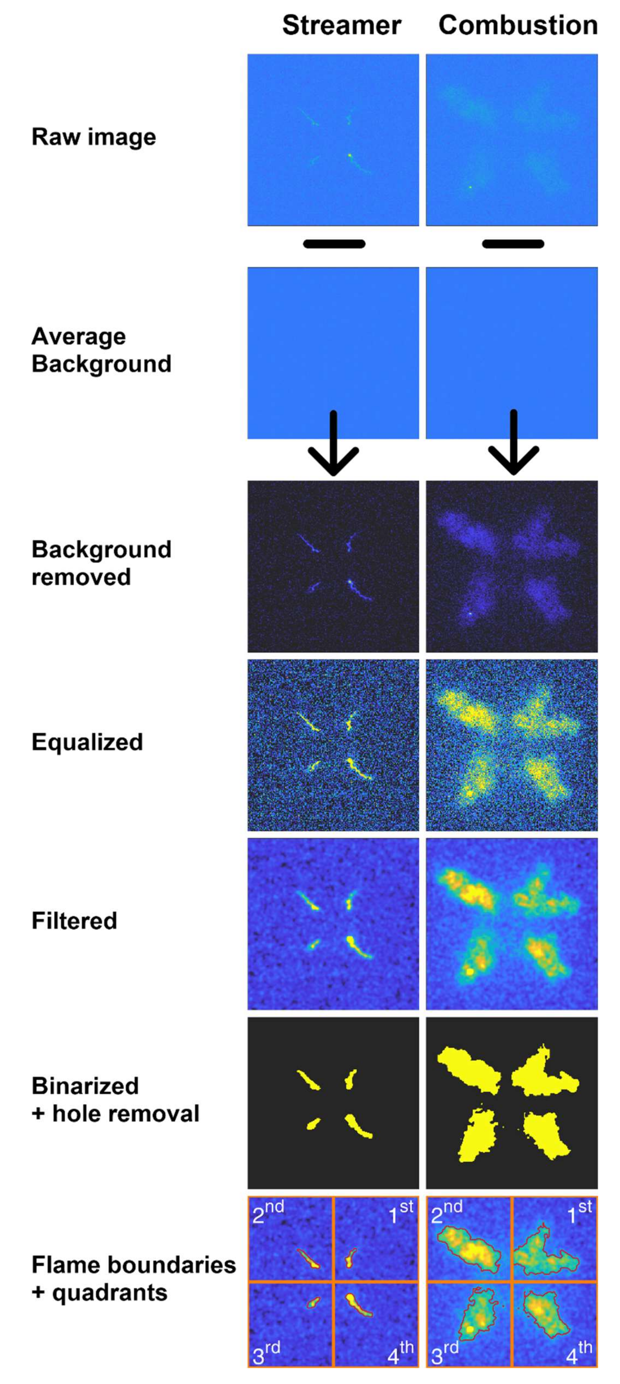
4.1.1. Average Background Computation and Removal, Equalization

Firstly, the background noise was characterized. Such noise was variable with time (Figure 6a), such that an average was necessary. The “average background” frame (BCK_avg) was generated by taking into account the gray level of the corresponding pixels of 20 frames before the discharge. Then, BCK_avg was subtracted from each discharge/combustion frame. As we can see from Figure 6b, the distribution of gray levels in the raw image belonged to the range 60–80 (black curve), while, after the background removal, such a distribution was much closer to zero (blue curve).

In order to improve the frame comprehensibility, an equalization was also performed. Gray levels were no longer displayed from 0–255 (maximum gray level with 8-bit resolution), but only up to 20. This choice was found to be effective at showing both dark and bright frames (e.g., the first discharge frames and a stoichiometric flame, respectively).

4.1.2. Filtering

A smoothing procedure was applied to each frame in order to reduce noise. For this purpose, a two-dimensional (2D) Gaussian filter (i.e., the MATLAB imgaussfilt built-in function) with a standard deviation of σ = 1.5 was used. This value, which belongs to a typical range that ensures effective Gaussian filtering [47], was found to be a good compromise between noise reduction and boundary conservation.

4.1.3. Thresholding and Binarization

With the described optical set-up, with such a high framerate and for the short period that was recorded, each filtered frame was characterized by a luminosity difference between discharge/combustion points and the other dark areas (Figure 5, “Filtered” row). The thresholding is the definition of a level above which a pixel is involved in streamer/flame and below which it is background. For all the test cases, the level choice was manual, in order to obtain results independently from a particular thresholding method. Note that, for the streamer analysis and for the first combustion frames, the selected threshold was pretty constant, in a level that ranged from 5–8 out of 255. This was found to be true for all the recorded series.

Upon defining the threshold level for each frame, the image was binarized, i.e., it was converted from grayscale to black and white (black means unburned or with no streamer, while white is the opposite).

From now on, the “binarized area” defines the group of white pixels.

4.1.4. Hole Filling

The MATLAB imfill built-in function allowed detecting holes in connected regions and removing them. Holes are non-binarized clusters of pixels completely surrounded by binarized ones. They do not represent a lack of streamer or flame; instead, they are the result of a missed binarization. Holes must be filled to correctly compute the binarized area.

4.1.5. Binarized Area Computation and Boundary Recognition

The binarized area was then computed by counting the number of white pixels for each black-and-white frame. Finally, the MATLAB bwboundaries built-in function was used to recognize the edges that separated under- and over-threshold pixels.

4.1.6. Quadrant Selection

In order to distinguish the different behavior of the streamers generated by the four-tip electrode, each frame was finally divided into four quadrants. Each quadrant was analyzed separately. The nomenclature used in this paper is the same as the Cartesian plane: the first quadrant is the top-right one, with the following quadrants in counter-clockwise order (Figure 5, last row).

4.2. Streamer Variability Calculation

For each quadrant, the calculation of the binarized area (i.e., the group of pixels related to the discharge) over time was performed. This was repeated over the different discharge events. For each frame, the algorithm evaluated the streamer penetration P, i.e., the maximum distance between the streamer and the corresponding tip from which it was generated. In Figure 7a, referred to as the first quadrant, as an example, the pixel which identifies the streamer penetration is marked with a white cross. This series of operations was repeated for each frame of the discharge sequence, and then for all the 63 consecutive events. In Figure 7b, for example, the trends of four discharges (among the 63) are shown. All the discharges started and ended at the same time, but the trend was found to be potentially different over the 63 events, particularly for the maximum streamer penetration P_max over a single discharge (colored circular marker). Note that the uncertainty in identifying the streamer penetration for each frame corresponded to ±1 pixel, i.e., 0.125 mm (according to Table 3), which is negligible if compared to the P_max values. In Figure 7c, the P_max for each discharge is shown. From this series, statistic parameters as the average (red dashed line) and standard deviation from the average (red dotted lines) were computed. Finally, the coefficient of variation (CoV) of the P_max, i.e., the ratio between standard deviation and average, was found.

Note that this method did not take into account the branching that potentially occurred; in every frame, only the farthest point in the entire quadrant was considered. Future work will be focused on shape detection, to improve this algorithm and make it robust for branching cases.

4.3. Streamer-to-Flame Transition Detection

The discharge in an air–fuel medium eventually results in flames. Intuitively, if we consider the streamer evolution in terms of overall luminosity (binarized area), we would expect a change in slope after the combustion initiation. When luminosity is generated only by the discharge, the initial rise in binarized area is limited, as the streamer is a sort of filament that involves a small number of pixels. Conversely, when the combustion starts, the pixels close to the filament are also involved, and the propagation is substantially perpendicular to the main streamer direction, obtaining a sort of lanceolate luminous area, which involves a large number of pixels.

Thus, theoretically, a discrimination of the combustion initiation could be possible by simply observing the binarized area evolution. Actually, this is not simple, since such area evolution is wobbly, showing a number of peaks and valleys. For example, in Figure 8a (second combustion event at λ = 1.0, first quadrant), many occurrences of slope change can be found. The corresponding smoothed series (red curve, temporal moving average with span = 5) shows the first increase in slope somewhere between 10 and 15 frames after the start of discharge, but exact detection is not easy. For all these reasons, this method requires a comparison with the corresponding data in motored conditions. As the discharge is a stochastic phenomenon, a statistical analysis was necessary; the average of all the discharge events in motored conditions was used to obtain the discharge trace for each tip (Figure 8b). Moreover, in many combustion cases, it was found that the streamer binarized area, before the flame kernel became visible, showed a sort of plateau, denoting that the maximum penetration was already reached (Figure 8a, frames in the range 11–13).

Thus, the detection of the streamer-to-flame transition was developed as follows:

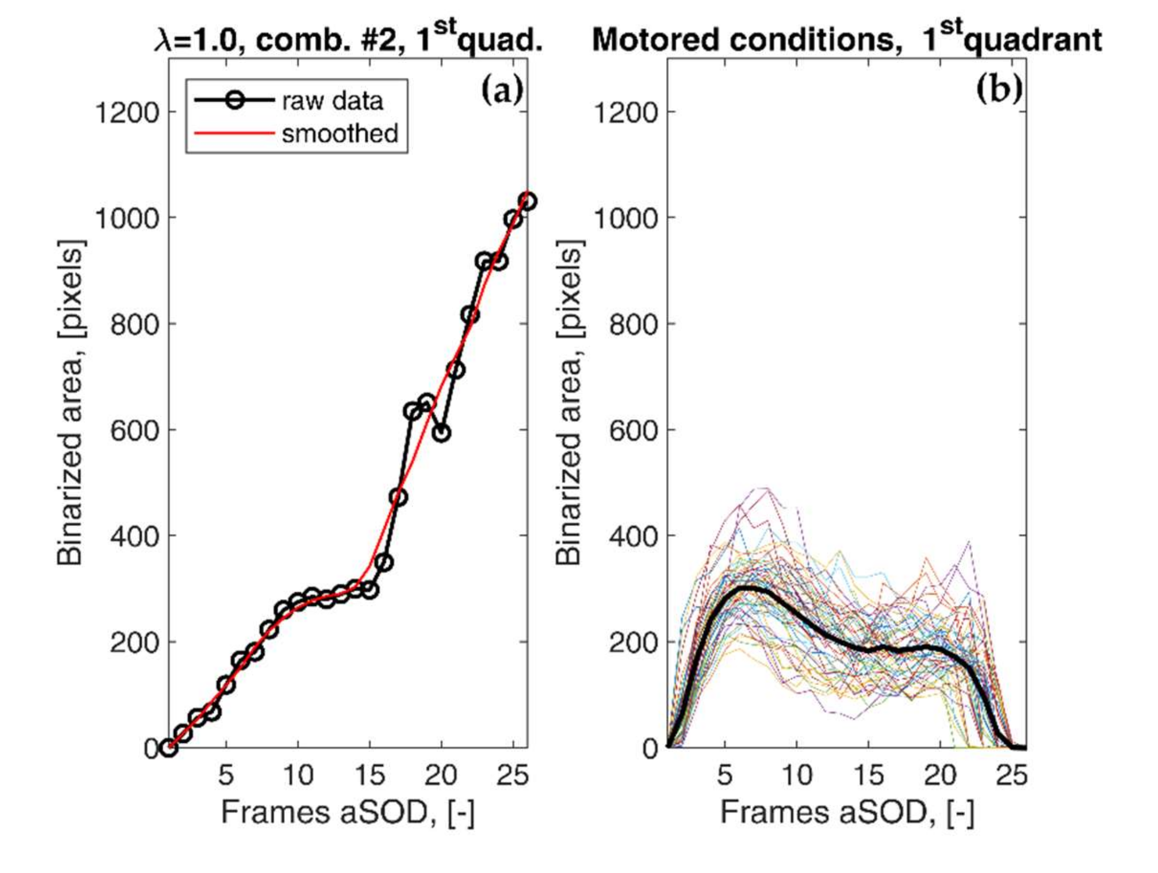
• For each combustion and for each quadrant, the binarized area trend was smoothed by using a five-point moving average. The five-point choice was found to be a good trade-off between the wobbly raw data and an even stronger smooth curve, which loses responsiveness.
• Once smoothed, the series was compared with the average trend in motored conditions (i.e., where no combustion occurs).
• The point of transition was determined by looking for a non-negligible increase in binarized area slope, which should occur in close proximity to the intersection between the combustion curve and the motored average one. After such a point, a region of strong increase in binarized area, not necessarily monotonic, should occur.

This procedure was applied and then visually tested on all the recorded series, for all the combustion events and all the quadrants. The visual test consisted of the observation of the streamer evolution frames, reported, as an example, in Figure 9 (second combustion, first quadrant, λ = 1.0). By simply observing this series, it can be stated that the very first frames had no combustion, while, in the last two rows, flames were certainly present. The red curve in Figure 10 represents the corresponding area evolution of Figure 9, and it allows a visual understanding of the described method. For such a red curve, this method indicated the 14th frame to be the transition one. As a further example, the blue curve (sixth combustion, first quadrant, λ = 1.4) shows the same trend, and the transition occurred in the 16th frame. Moreover, this picture allowed noting a different behavior between red and blue cases; after flame onset, the binarized area for the red case continued to grow, while that in the blue one reached a sort of plateau after the 20th frame. This behavior was found to be recurrent for the lean cases and related more to flame propagation than to the flame onset. The subsequent flame kernel evolution was investigated in other works [15,32].

It is worth mentioning that this method, even if maintaining a degree of uncertainty, strongly restricted, to a few frames, the range in which the streamer-to-flame transition occurred; an uncertainty of three frames denotes less than 0.25 CAD.

5. Results and Discussion

5.1. Streamer Variability

Figure 11 Shows, at a glance, the cycle-by-cycle streamer dispersion in motored conditions. It contains the points of maximum penetration for all the recorded engine cycles, all in the same picture for the sake of comprehensibility. The corresponding quantitative results can be found in

Table 5. P_max statistic results: series average, series standard deviation, and series coefficient of variation for the four quadrants.

Feature	Unit	1st quadrant	2nd quadrant	3rd quadrant	4th quadrant
Series average	mm	5.87	4.15	4.11	7.27
Series standard deviation	mm	1.02	0.947	0.911	0.994
Series CoV	%	17.4	22.8	22.1	13.7

. In Figure 12, the sequence of all P_max values can be found, together with a visualization of average and standard deviation for each quadrant. From this figure, it can be stated that there is not a time-dependent trend; thus, the previous cycle seems not to affect the max penetration of the following one. In the tested operating condition, streamers coming from the fourth quadrant tip were, on average, the longest (about 7 mm), while those from the second and third quadrants were the shortest (about 4 mm). It is worth noting that the corresponding penetration standard deviation was not so different among the tips, ranging from 0.9 to 1.0 mm. This resulted in a coefficient of variation of such penetration that, for the fourth tip, was the lowest, while that for the second and third ones was the highest.

In future work, further analysis will be carried out to determine if such a distribution was due to the features of the igniter or to the conditions in the combustion chamber, i.e., if a change in the igniter orientation would affect such variability. For example, it can be noted that the first and the fourth tips, which featured the highest P_max on average, were the closest to the engine intake valves, while the second and third tips were the closest to the exhaust side. This observation will be evaluated in future experimental campaigns, in order to investigate whether in-cylinder flow motion is responsible for this asymmetry. Sensitivity to V_d and T_d will be analyzed as well, with the methodology here presented.

Finally, this method did not take into account the angular position of the maximum penetration; two streamers which penetrated up to the same distance from the same tip, but with a different orientation, were equivalent in this code. In future developments, we will also evaluate such parameters. Nevertheless, it can be considered of second order; generally speaking, a higher penetration resulted in a higher radical insemination and greater released thermal energy [34,48], along with a more effective combustion [17], independently of the orientation.

5.2. Streamer-to-Flame Transition

With the method described in the previous sections, the distribution with lambda of the time to obtain visible flames after the start of discharge was found, as can be seen in Figure 13. Firstly, in each of the tested cases, a visible flame was generated before the end of the discharge. On average, at λ = 1.0, flames appeared between the 12th and 13th frames after the discharge start; at λ = 1.2, they appeared between the 13th and the 15th frames, while, in the λ = 1.4 case, they appeared between the 14th and the 15th frames. Note that such values refer to the average, while the standard deviation, not reported in the graph, was found to be pretty constant, i.e., between 1.7 and 2.3 for all cases. Focusing on each quadrant, a monotonic non-decreasing relationship between lambda and the transition average frame was found.

It is worth remarking that the difference of max three frames denotes about 0.23 CAD; whatever the tested lambda, the corona igniter was able to ignite the mixture proficiently, before the end of the discharge. These results assess the corona effectiveness in terms of quickness in flame kernel generation, as well as with moderate and medium/lean mixtures [15]. Note that no further information regarding combustion evolution was provided from the optical point of view, since this analysis was focused on the flame onset detection. Such results can be found in other works [11,14,15,32].

Finally, at constant lambda, no relationships were found between streamer variability in motored conditions and the transition frame. This means that, despite a certain variability in the streamers generated from each tip, the discharge mechanism was effective, thanks to the combined thermal and chemical effects [17,34]. The streamer variability, instead, was one of the factors responsible for the engine CCV, with a strong effect, particularly in the first 5% of MFB [32], which can be investigated with other optical techniques such as the flame probability presence [49].

6. Conclusions

In this work, an optical method was presented to characterize the radio-frequency corona streamer penetration variability and the transition from streamer to flame in an optical engine. For this purpose, a high-speed camera able to record the natural luminosity of discharge and combustion in the visible range was used. Framerate and frame area were set to ensure high temporal resolution (79 kHz) and high magnification, respectively, to properly analyze such phenomena. Engine speed and throttle position, together with corona electrical parameters, were fixed to ensure high repeatability in terms of in-cylinder conditions and power supply at the igniter electrode. Streamer penetration was calculated in motored conditions, while streamer-to-flame transition was recorded with three different fueling levels, to ensure a relative air–fuel ratio λ of 1.0, 1.2, and 1.4.

The main findings are as follows:

• A stable preprocessing method was determined, based on in-house MATLAB scripts together with built-in functions. It consisted of average background removal, equalization, Gaussian filtering, and thresholding. The threshold level was defined manually, frame by frame, but the threshold level to discriminate dark and light pixels belonged to an easily detectable narrow range. The procedure continued with binarization, hole filling, and boundary recognition. Finally, the frame area was divided into four quadrants, in order to analyze the discharge events from the corona tips independently from each other.
• A method to evaluate streamer repeatability in motored conditions was reported. For each discharge event, the maximum penetration (i.e., the maximum distance between streamer and tip) over time was detected. The maxima values, one for each consecutive discharge, were compared, and a statistical analysis was carried out, where the average value, standard deviation, and coefficient of variation were computed. This procedure was carried out separately for each igniter tip.
• A method to discriminate frames with pure streamer from combustion frames was reported. It was based on the evolution of the binarized area, evaluated separately for each electrode tip. The first significant increase in slope that generated a deviation between the binarized area trend and the corresponding motored one was defined as the detection condition for the flame presence.
• For the motored test case, as an example, the streamer penetration parameters were calculated. According to the nomenclature used in this work, the highest streamer penetration, on average, was found for the fourth tip (more than 7 mm), while the second and third tips featured with the lowest penetration (about 4 mm). Standard deviation, on the contrary, was not so different among the four tips (0.9–1.0 mm).
• By applying the method to detect the transition between streamer and flames, it was found that all visible flames were always present at the end of the discharge. On average, at fixed lambda, it was not possible to find a tip-dependent trend. Focusing on the tip, instead, a lower lambda resulted in more advanced early flame detection. Nevertheless, the average gap in the first frame with combustion between the three lambda values was small (at most three frames, i.e., about 0.2 crank angle degrees).

References

1. Thangaraja, J.; Kannan, C. Effect of Exhaust Gas Recirculation on Advanced Diesel Combustion and Alternate Fuels—A Review. Appl. Energy 2016, 180, 169–184. [Google Scholar] [CrossRef]
2. Battistoni, M.; Grimaldi, C.N.; Cruccolini, V.; Discepoli, G.; De Cesare, M. Assessment of Port Water Injection Strategies to Control Knock in a GDI Engine through Multi-Cycle CFD Simulations. SAE Tech. Pap. 2017, 14. [Google Scholar] [CrossRef]
3. Nakata, K.; Nogawa, S.; Takahashi, D.; Yoshihara, Y.; Kumagai, A.; Suzuki, T. Engine Technologies for Achieving 45% Thermal Efficiency of S.I. Engine. SAE Int. J. Engines 2015, 9. [Google Scholar] [CrossRef]
4. Huang, S.; Zhang, Z.; Song, H.; Wu, Y.; Li, Y. A Novel Way to Enhance the Spark Plasma-Assisted Ignition for an Aero-Engine Under Low Pressure. Appl. Sci. 2018, 8, 1533. [Google Scholar] [CrossRef] [Green Version]
5. Zembi, J.; Mariani, F.; Battistoni, M. Large Eddy Simulation of Ignition and Combustion Stability in a Lean SI Optical Access Engine. SAE Tech. Pap. 2019, 13. [Google Scholar] [CrossRef]
6. Scarcelli, R.; Zhang, A.; Wallner, T.; Breden, D.; Karpatne, A.; Raja, L.; Ekoto, I.; Wolk, B. Multi-dimensional Modeling of Non-equilibrium Plasma for Automotive Applications. SAE Tech. Pap. 2018, 1–10. [Google Scholar] [CrossRef]
7. Nishiyama, A.; Le, M.K.; Furui, T.; Ikeda, Y. The Relationship between In-Cylinder Flow-Field near Spark Plug Areas, the Spark Behavior, and the Combustion Performance inside an Optical S.I. Engine. Appl. Sci. 2019, 9, 1545. [Google Scholar] [CrossRef] [Green Version]
8. Breden, D.; Karpatne, A.; Suzuki, K.; Raja, L. High-Fidelity Numerical Modeling of Spark Plug Erosion. SAE Tech. Pap. Ser. 2019, 1, 1–12. [Google Scholar] [CrossRef]
9. Yang, Z.; Yu, X.; Yu, S.; Han, X.; Tan, Q.; Chen, G.; Chen, X.; Zheng, M. Effects of Spark Discharge Energy Scheduling on Flame Kernel Formation under Quiescent and Flow Conditions. SAE Tech. Pap. 2019, 1–11. [Google Scholar] [CrossRef]
10. Shiraishi, T.; Urushihara, T.; Gundersen, M. A trial of ignition innovation of gasoline engine by nanosecond pulsed low temperature plasma ignition. J. Phys. D Appl. Phys. 2009, 42, 135208. [Google Scholar] [CrossRef]
11. Cruccolini, V.; Discepoli, G.; Cimarello, A.; Battistoni, M.; Mariani, F.; Grimaldi, C.N.; Dal Re, M.A. Lean combustion analysis using a corona discharge igniter in an optical engine fueled with methane and a hydrogen-methane blend. Fuel 2020, 259, 116290. [Google Scholar] [CrossRef]
12. Idicheria, C.A.; Yun, H.; Najt, P.M. An Advanced Ignition System for High Efficiency Engines. In Ignition Systems for Gasoline Engines, Proceedings of the 4th International Conference, Berlin, Germany, 6–7 December 2018; Expert Verlag: Tübingen, Germany, 2018; pp. 40–54. [Google Scholar] [CrossRef]
13. Kuramochi, A.; Takahashi, E.; Asakawa, D.; Saito, N.; Nishioka, M. Flame Propagation Enhancement by Dielectric Barrier Discharge-Generated Intermediate Species. Combust. Sci. Technol. 2019, 191, 1972–1989. [Google Scholar] [CrossRef]
14. Marko, F.; König, G.; Schöffler, T.; Bohne, S.; Dinkelacker, F. Comparative Optical and Thermodynamic Investigations of High Frequency Corona- and Spark-Ignition on a CV Natural Gas Research Engine Operated with Charge Dilution by Exhaust Gas Recirculation. In Ignition Systems for Gasoline Engines; Springer International Publishing: Cham, Switzerland, 2017; pp. 293–314. ISBN 978-3-319-45503-7. [Google Scholar] [CrossRef]
15. Cimarello, A.; Grimaldi, C.N.; Mariani, F.; Battistoni, M.; Dal Re, M. Analysis of RF Corona Ignition in Lean Operating Conditions Using an Optical Access Engine. SAE Tech. Pap. 2017, 16. [Google Scholar] [CrossRef]
16. Merola, S.S.; Marchitto, L.; Tornatore, C.; Valentino, G.; Irimescu, A. Optical Characterization of Combustion Processes in a DISI Engine Equipped with Plasma-Assisted Ignition System. Appl. Therm. Eng. 2014, 69, 177–187. [Google Scholar] [CrossRef]
17. Ju, Y.; Sun, W. Plasma assisted combustion: Dynamics and chemistry. Prog. Energy Combust. Sci. 2015, 48, 21–83. [Google Scholar] [CrossRef]
18. Pineda, D.I.; Wolk, B.; Chen, J.-Y.; Dibble, R.W. Application of Corona Discharge Ignition in a Boosted Direct-Injection Single Cylinder Gasoline Engine: Effects on Combustion Phasing, Fuel Consumption, and Emissions. SAE Int. J. Engines 2016, 9. [Google Scholar] [CrossRef]
19. Burrows, J.; Mixell, K.; Reinicke, P.B.; Riess, M.; Sens, M. Corona Ignition—Assessment of Physical Effects by Pressure Chamber, Rapid Compression Machine, and Single Cylinder Engine Testing. In Ignition Systems for Gasoline Engines, Proceedings of the 2nd International Conference; Berlin, Germany, 24–25 November 2014, pp. 87–107. ISBN 9783944976228.
20. Burrows, J.; Mixell, K. Analytical and Experimental Optimization of the Advanced Corona Ignition System. In Ignition Systems for Gasoline Engines; Springer International Publishing: Cham, Switzerland, 2016; pp. 267–292. [Google Scholar] [CrossRef]
21. Discepoli, G.; Cruccolini, V.; Ricci, F.; Di Giuseppe, A.; Papi, S.; Grimaldi, C.N. Experimental characterisation of the thermal energy released by a Radio-Frequency Corona Igniter in nitrogen and air. Appl. Energy 2020, 263, 114617. [Google Scholar] [CrossRef] [Green Version]
22. Suess, M.; Guenthner, M.; Schenk, M.; Rottengruber, H. Investigation of the Potential of Corona Ignition to Control Gasoline Homogeneous Charge Compression Ignition Combustion. Proc. Inst. Mech. Eng. Part D J. Automob. Eng. 2012, 226, 275–286. [Google Scholar] [CrossRef]
23. Pastor, J.; Olmeda, P.; Martín, J.; Lewiski, F. Methodology for Optical Engine Characterization by Means of the Combination of Experimental and Modeling Techniques. Appl. Sci. 2018, 8, 2571. [Google Scholar] [CrossRef] [Green Version]
24. Koegl, M.; Baderschneider, K.; Bauer, F.J.; Hofbeck, B.; Berrocal, E.; Will, S.; Zigan, L. Analysis of the LIF/Mie Ratio from Individual Droplets for Planar Droplet Sizing: Application to Gasoline Fuels and Their Mixtures with Ethanol. Appl. Sci. 2019, 9, 4900. [Google Scholar] [CrossRef] [Green Version]
25. Nishiyama, A.; Le, M.K.; Furui, T.; Ikeda, Y. Simultaneous In-Cylinder Flow Measurement and Flame Imaging in a Realistic Operating Engine Environment Using High-Speed PIV. Appl. Sci. 2019, 9, 2678. [Google Scholar] [CrossRef] [Green Version]
26. Martinez, S.; Merola, S.; Irimescu, A. Flame Front and Burned Gas Characteristics for Different Split Injection Ratios and Phasing in an Optical GDI Engine. Appl. Sci. 2019, 9, 449. [Google Scholar] [CrossRef] [Green Version]
27. Irimescu, A.; Marchitto, L.; Merola, S.S.; Tornatore, C.; Valentino, G. Evaluation of Different Methods for Combined Thermodynamic and Optical Analysis of Combustion in Spark Ignition Engines. Energy Convers. Manag. 2014, 87, 914–927. [Google Scholar] [CrossRef]
28. Michalski, Q.; Benito Parejo, C.J.; Claverie, A.; Sotton, J.S.; Bellenoue, M. An Application of Speckle-Based Background Oriented Schlieren for Optical Calorimetry. Exp. Therm. Fluid Sci. 2018, 91, 470–478. [Google Scholar] [CrossRef]
29. Sun, L.; Meng, X.; Xu, J.; Tian, Y. An Image Segmentation Method Using an Active Contour Model Based on Improved SPF and LIF. Appl. Sci. 2018, 8, 2576. [Google Scholar] [CrossRef] [Green Version]
30. Otsu, N. A Threshold Selection Method from Gray-Level Histograms. IEEE Trans. Syst. Man Cybern. 1979, 9, 62–66. [Google Scholar] [CrossRef] [Green Version]
31. Shawal, S.; Goschutz, M.; Schild, M.; Kaiser, S.A.; Neurohr, M.; Pfeil, J.; Koch, T. High-Speed Imaging of Early Flame Growth in Spark-Ignited Engines Using Different Imaging Systems via Endoscopic and Full Optical Access. SAE Int. J. Engines 2016, 9. [Google Scholar] [CrossRef]
32. Cimarello, A.; Cruccolini, V.; Discepoli, G.; Battistoni, M.; Mariani, F.; Grimaldi, C.N.; Dal Re, M. Combustion Behavior of an RF Corona Ignition System with Different Control Strategies. SAE Tech. Pap. 2018, 1–19. [Google Scholar] [CrossRef]
33. Cruccolini, V.; Discepoli, G.; Ricci, F.; Petrucci, L.; Grimaldi, C.N.; Papi, S.; Dal Re, M. Comparative Analysis between a Barrier Discharge Igniter and a Streamer-type Radio-Frequency Corona Igniter in an Optically Accessible Engine in Lean Operating Conditions. SAE Tech. Pap. 2020, 12. [Google Scholar] [CrossRef]
34. Discepoli, G.; Cruccolini, V.; Dal Re, M.; Zembi, J.; Battistoni, M.; Mariani, F.; Grimaldi, C.N. Experimental Assessment of Spark and Corona Igniters Energy Release. Energy Procedia 2018, 148, 1262–1269. [Google Scholar] [CrossRef]
35. Loeb, L.B. Electrical Coronas: Their Basic Physical Mechanisms; University of California Press: Berkeley, CA, USA, 1965; ISBN 9780520007659. [Google Scholar]
36. Scarcelli, R.; Wallner, T.; Som, S.; Biswas, S.; Ekoto, I.; Breden, D.; Karpatne, A.; Raja, L. Modeling Non-Equilibrium Discharge and Validating Transient Plasma Characteristics at Above-Atmospheric Pressure. Plasma Source Sci. Technol. 2018, 27, 124006. [Google Scholar] [CrossRef]
37. Qin, J.; Pasko, V.P. On the propagation of streamers in electrical discharges. J. Phys. D Appl. Phys. 2014, 47, 435202. [Google Scholar] [CrossRef]
38. Ricci, F.; Zembi, J.; Battistoni, M.; Grimaldi, C.N.; Discepoli, G.; Petrucci, L. Experimental and Numerical Investigations of the Early Flame Development Produced by a Corona Igniter. SAE Tech. Pap. Ser. 2019, 12. [Google Scholar] [CrossRef]
39. Bhatti, S.S.; Verma, S.; Tyagi, S.K. Energy and Exergy Based Performance Evaluation of Variable Compression Ratio Spark Ignition Engine Based on Experimental Work. Therm. Sci. Eng. Prog. 2019, 9, 332–339. [Google Scholar] [CrossRef]
40. Terry, O.; Rochussen, J.; Kirchen, P. Development of a Modular, Dry-Running Bowditch Piston with Efficient Window Cleaning. SAE Tech. Pap. 2018, 1–14. [Google Scholar] [CrossRef]
41. Irimescu, A.; Tornatore, C.; Marchitto, L.; Merola, S.S. Compression Ratio and Blow-By Rates Estimation Based on Motored Pressure Trace Analysis for an Optical Spark Ignition Engine. Appl. Therm. Eng. 2013, 61, 101–109. [Google Scholar] [CrossRef]
42. SAE J1832_200102, Low Pressure Gasoline Fuel Injector, SAE International Standard; SAE International: Warrendale, PA, USA, 2001. [CrossRef]
43. Phantom V71X—Color & Spectral Response Curve. Available online: https://www.phantomhighspeed.com/products/cameras/vseries/v711 (accessed on 15 January 2020).
44. Romani, L.; Bianchini, A.; Vichi, G.; Bellissima, A.; Ferrara, G. Experimental Assessment of a Methodology for the Indirect in-Cylinder Pressure Evaluation in Four-Stroke Internal Combustion Engines. Energies 2018, 11, 1982. [Google Scholar] [CrossRef] [Green Version]
45. Ganesh, S.; Rajabooshanam, A.; Dhali, S.K. Numerical Studies of Streamer to Arc Transition. J. Appl. Phys. 1922, 72, 3957–3965. [Google Scholar] [CrossRef]
46. Kuffel, E.; Kuffel, J. High Voltage Engineering Fundamentals, 2nd ed.; Elsevier: Oxford, UK, 2000; ISBN 9780750636346. [Google Scholar] [CrossRef]
47. Semmlow, J. Two-Dimensional Signals—Basic Image Analysis. In Circuits, Signals and Systems for Bioengineers; Academic Press: Cambridge, MA, USA, 2018; pp. 491–526. [Google Scholar] [CrossRef]
48. Wolk, B.M.; Ekoto, I. Calorimetry and Imaging of Plasma Produced by a Pulsed Nanosecond Discharge Igniter in EGR Gases at Engine-Relevant Densities. SAE Int. J. Engines 2017, 10. [Google Scholar] [CrossRef]
49. Aleiferis, P.G.; Serras-Pereira, J.; Richardson, D. Characterisation of Flame Development with Ethanol, Butanol, Iso-Octane, Gasoline and Methane in a Direct-Injection Spark-Ignition Engine. Fuel 2013, 109, 256–278. [Google Scholar] [CrossRef] [Green Version]
Figure 1. (a) Test engine; (b) details of engine head.
Applsci 10 02275 g001
Figure 2. (a) Details of Bowditch piston and optical access; (b) Advanced Corona Ignition System (ACIS) igniter, with an example of discharge in air.
Applsci 10 02275 g002
Figure 3. Schematic of measurement apparatus.
Applsci 10 02275 g003
Figure 4. Pressure traces averaged on 101 consecutive cycles. For all cases, the ignition timing (IT) was 20 CAD bTDC (gray line), with Vd = 28 V and Td = 300 μs.
Applsci 10 02275 g004
Figure 5. Preliminary preprocessing procedure, common for “pure streamer” frames (left column) and combustion frames (right column).
Applsci 10 02275 g005
Figure 6. (a) Gray level, evaluated over time, during the average background computation. The pink curve refers to a single pixel, e.g., that in the center of the frame. The green curve is the average gray value over the entire 256 × 256 pixel frame. (b) Histogram of gray levels for a raw frame (black) and the corresponding histogram after background removal (blue).
Applsci 10 02275 g006
Figure 7. Example to explain the coefficient of variation (CoV) streamer calculation methodology. All pictures refer to the first quadrant. (a) Streamer penetration P detection. The red asterisk represents the igniter tip position, while the white cross represents the streamer’s farthest point. (b) Temporal evolution of the penetration P for a certain number of streamers. Each streamer sequence is defined by a different line type; circular colored markers represent the point of maximum penetration Pmax for each sequence of frames. All the streamers start at the same time, but the Pmax and trend can be fairly different. (c) Maximum streamer penetration Pmax trend over the series of 63 consecutive discharges. The red dashed line represents the average value (avg). Red dotted lines represent the series standard deviation (±devstd) from the corresponding average value.
Applsci 10 02275 g007
Figure 8. (a) Example of binarized area evolution during combustion (λ = 1.0, combustion #2, first quadrant); (b) binarized area in motored conditions. Colored curves refer to each single discharge event; the black curve is the corresponding average.
Applsci 10 02275 g008
Figure 9. Streamer evolution for λ = 1.0, combustion #2, first quadrant. The igniter is in the bottom-left corner. The numbers above each picture refer to the corresponding frames from the start of discharge. Streamer-to-flame transition occurs at the 14th frame after the start of discharge, according to the method presented in this section.
Applsci 10 02275 g009
Figure 10. Binarized area during the discharge/combustion event, first quadrant. Black dotted lines refer to each discharge event in motored conditions (no combustion), and the black solid line is their average. Red and blue dashed curves with markers are, respectively, the curves corresponding to the λ = 1.0 second event and the λ = 1.4 sixth event, as examples. Finally, red and blue solid lines are the corresponding smoothed curves (five-point moving average). For both combustion cases, we would expect a visible flame kernel in the narrow range between the 13th and the 16th frame after the start of discharge (aSOD; green ellipse).
Applsci 10 02275 g010
Figure 11. Max penetration distribution of streamers in the four quadrants. The white cross in the middle is the igniter center. The discharge in the background is only for the sake of comprehensibility.
Applsci 10 02275 g011
Figure 12. Details of max penetration distribution for the four quadrants over the 63 consecutive discharges. White-filled circles represent the single events, while dashed lines represent the series average value (avg) for each quadrant. Dotted lines represent the series standard deviation (±devstd) from the corresponding average value.
Applsci 10 02275 g012
Figure 13. Distribution of the frame aSOD in which streamer-to-flame transition occurs. Bars refer to the average value (among the 63 events recorded for each test case).
Applsci 10 02275 g013