Assessment of the Algorithm for Single Frequency Precise Point Positioning at Different Latitudes and with Distinct Magnetic Storm Conditions

Abstract

This paper analyzes the convergence time and the root mean square (RMS) error of single frequency (SF) precise point positioning (PPP) in the ionospheric-constrained (TIC1) and troposphere- and ionospheric-constrained (TIC2) conditions, when the stations are at a low latitude, mid-latitude, and high latitude area during the period of a magnetic storm (MS) and a non-magnetic storm (NMS). In this paper, 375 IGS (international global navigation satellite system (GNSS) service) stations were selected from all over the world for 30 days in September 2017. The 24 hour daily observations were split for each station into 8 data sets of 3 hours each, so that a total of 90,000 tests were carried out. After statistical analysis, it was concluded that: during the MS period, the percentage of TIC2 shortened compared to the TIC1 convergence time, and it was by at least 3.9%, 3.0%, and 9.3% when the station was at global, low latitude, and high latitude areas, respectively. According to the statistical analysis, during the NMS period the convergence time was shortened about at least 12.8%, 11.0%, and 30.0% with respect to the stations in the MS period at global, low, and high latitude areas, respectively. If the station was located in the mid-latitude region, the convergence time was not shortened in some modes. The ionospheric activity in the mid-latitude region was less than that in the low-latitude region, while there were more stations in the mid-latitude region, and the precision of the global ionospheric maps (GIMs) and zenith tropospheric delay (ZTD) products were also slightly higher. Overall, TIC1 and TIC2 have a greater impact on convergence time, but have less impact on positioning accuracy, and only have a greater impact in different environments during the MS and NMS periods.

1. Introduction

With respect to signal propagation, the atmosphere is subdivided into two main layers of the troposphere (also referred to as neutral atmosphere) and the ionosphere. When satellite signals pass through the atmosphere and reach the receiver antenna, the satellite electromagnetic signal will be delayed. The delay can be divided into ionospheric delay and tropospheric delay. Ionospheric delay and tropospheric delay can result in distance errors for international global navigation satellite system (GNSS) satellite users who require high precision measurements [1]. In the case of severe ionospheric disturbances, the pseudorange measurement error increases to about 100 meters [2]. The tropospheric delay contains a hydrostatic component and a wet component. In the zenith direction, the hydrostatic component reaches around 2.3 m [3,4] and the wet component varies from centimeters (or less) in the arid regions to as large as 0.35 m in the humid regions [3,5]. Therefore, for precise point positioning (PPP), it is necessary to correct these two delays. Using the global ionospheric maps (GIMs) and tropospheric zenith path delays announced by the international global navigation satellite system (GNSS) service (IGS) can improve the GNSS positioning performance.

In 1998, the IGS organization established an ionospheric working group to continuously monitor ionospheric changes and provide daily GIMs products with a standard deviation of 2-8 TECU (total electron content units) [6]. For dual-frequency precise point positioning (PPP), the ionospheric-free (IF) combination can be used to eliminate the influence of the first order term of the ionospheric delay [7], but the noise is amplified, and the ionospheric delay is solved as a parameter by undifferentiated and uncombined analysis, then avoiding the noise amplification [8]. Of course, it is also possible to estimate the ionospheric delay by using a prior ionospheric model [9,10]. Reference [11] through experimental analysis shows that by using constraint through GIMs products the convergence time of dual-frequency PPP is reduced by 30%. Reference [12,13] applied ionospheric-constrained to inertial navigation system (INS) assisted PPP to overcome the adverse effects of PPP in kinematic mode. Compared with dual-frequency PPP, single-frequency (SF) PPP has received more attention due to its low cost, but ionospheric delay is still the main error. Similar to the dual-frequency (DF) IF, the single-frequency (SF) observation also has an IF combination. The SF IF is a combination between the code and carrier phase observations, which is called group and phase ionospheric correction (GRAPHIC) [14,15,16]. Based on GRAPHIC, the positioning accuracy of SF PPP can be improved, but the convergence time is extended. Several scholars use GIMs constraints in single-frequency PPP to reduce convergence time [10,17,18,19]. However, they did not mention the influence of tropospheric constraints on SF PPP convergence time.

Some scholars have studied tropospheric constraints. Reference [20] developed a new global positioning system (GPS)/Beidou navigation satellite system (BDS) real time kinematic (RTK) algorithm that is constrained by tropospheric delay parameters from a numerical weather prediction (NWP) model for medium/long-range baselines, which is better than 3 cm in the horizontal component and better than 5 cm in the vertical component. Reference [21] developed a numerical weather model (NWM)-constrained PPP processing system to improve the multi-GNSS PPP, and with the NWM-constrained, the convergence time was shortened by 20.0%, 32.0%, and 25.0% for the north, east, and vertical components, respectively. After the troposphere constraint was used for the fixed PPP/INS adaptive covariance model to converge for one hour, the positional accuracy of the north, east, and height components were increased by 19.51%, 61.11%, and 23.53%, respectively, compared with the conventional PPP solution [22]. Constraining the atmospheric, reference [23] had studied the positioning accuracy and convergence time in dual- and triple-frequency PPP. It was verified that the accuracy of triple-frequency positioning was improved by 60% more than dual-frequency under atmospheric-constrained conditions.

In this paper, the influence of SF PPP on positioning accuracy and convergence time under ionospheric-constrained (TIC1) and troposphere- and ionospheric-constrained (TIC2) conditions are studied. The difference between positioning accuracy and convergence time of the station in the period of magnetic storms (MS) and non-magnetic storms (NMS) and geography at different latitudes are analyzed. The organization of the paper is as follows: the introduction is in Section 1, mathematical models are in Section 2, data sets and processing strategy are in Section 3, results and discussion are in Section 4, and conclusions are in Section 5.

2. Methodology

The linearization of the pseudorange and carrier phase observation equations containing the parameters to be sought can be expressed as [24]:

$$p_{r,1}^s={\mathsf{\mu }}_r^s·\mathit{x}+d{t}_r-d{t}^s+V_{r,trop}^s+I_{r,1}^s+(d_{r,1}-d_1^s)$$

(1)

$$l_{r,1}^s={\mathsf{\mu }}_r^s·\mathit{x}+d{t}_r-d{t}^s+V_{r,trop}^s-I_{r,1}^s+{\lambda }_1^s·(N_{r,1}^s+b_{r,1}-b_1^s)$$

(2)

where $s$ indicates satellite; $r$ represents the receiver; $p_{r,1}^s$ and $l_{r,1}^s$ denote observed minus computed (OMC) values of the pseudorange and carrier phase observables on the first frequency, respectively; ${\mathsf{\mu }}_r^s$ represents the unit vector from the satellite to the receiver; $\mathit{x}$ is the vector of the receiver position increments relative to the a priori position; $d{t}_r$ and $d{t}^s$ are the clock bias of the receiver and satellite, respectively; $V_{r,trop}^s$ is the troposphere delay; $I_{r,1}^s$ is the slant ionospheric delay on the first frequency ${\mathrm{f}}_1$; $d_{r,1}$ is the frequency-dependent receiver uncalibrated code delay (UCD) with respect to satellite $s$; $d_1^s$ is the frequency-dependent satellite UCD; $N_{r,1}^s$ is the integer phase ambiguity; $b_{r,1}$ and $b_1^s$ are the uncalibrated phase delays (UPDs) for the receiver and satellite, frequency-dependent.

In order to speed up the convergence, the GIMs product provided by IGS can be used as a pseudo-observation to constrain the ionospheric delay. The mathematical model can be written as:

$$I_{r,GIM}^s=I_{r,1,GIM}^s+{\epsilon }_{GIM},\begin{array}{ccc}& {\epsilon }_{GIM}\in N(0,{\sigma }_{GIM}^2)& \end{array}$$

(3)

where $I_{r,1,GIM}^s$ is calculated from the GIMs product value and the ionosphere pierce point (IPP) angle [25]; ${\sigma }_{GIM}^2$ is a priori variance for the noise ${\epsilon }_{GIM}$ of the GIMs product.

Then the ionospheric delay correction ($v_I$) equation is:

$$v_I=I_{r,GIM}^s-I_r^s$$

(4)

IGS also provides tropospheric delay products (i.e., zenith tropospheric delay, ZTD), which can be used as a constraint, and expressed as:

$$V_{r,ZTD}^s=V_{r,1,ZTD}^s+{\epsilon }_{ZTD},\begin{array}{ccc}& {\epsilon }_{ZTD}\in N(0,{\sigma }_{ZTD}^2)& \end{array}$$

(5)

where $V_{r,1,ZTD}^s$ can be expressed as a ZTD value and mapping function [26], ${\sigma }_{ZTD}^2$ is a priori variance for its noise ${\epsilon }_{ZTD}$ of the ZTD product.

Then the tropospheric delay correction ($v_T$) equation is:

$$v_T=V_{r,ZTD}^s-V_{r,trop}^s$$

(6)

The Kalman filtering method [27] is a parameter estimation method proposed by Kalman around 1960. The method predicts the state of the next moment by the noise of the measurement and state vector at the priori moment. The true value of the current moment is estimated more accurately by observing the noise and the estimated noise. For the GNSS raw observations (pseudorange and carrier phase), the observation model can be expressed as:

$${\mathit{Z}}_{k+1}={\mathit{H}}_{k+1}{\mathit{X}}_{k+1}+{\upsilon }_{k+1},\begin{array}{ccc}& {\upsilon }_{k+1}\in N(0,{\mathit{R}}_{k+1})& \end{array}$$

(7)

where ${\mathit{Z}}_{k+1}$ is the vector of measurements at epoch $k+1$ of the GNSS raw observations; ${\mathit{H}}_{k+1}$ is the design matrix; vector ${\mathit{X}}_{k+1}$ represents the parameters; ${\upsilon }_{k+1}$ represents the observation noise with the priori covariance matrix ${\mathit{R}}_{k+1}$. For single-frequency observations, the ${\mathit{Z}}_{k+1}$ can be written as:

$${\mathit{Z}}_{k+1}=\left[\begin{array}{c}{p}_{r,1}^s\\ l_{r,1}^s\end{array}\right]+\left[\begin{array}{c}{\upsilon }_{p_1}\\ {\upsilon }_{l_1}\end{array}\right]$$

(8)

where ${\upsilon }_{p_1}$ represents the pseudorange observation noise; ${\upsilon }_{l_1}$ represents the carrier phase observation noise.

According to the mathematical functions above, the state parameter vector ${\mathit{X}}_{k+1}$ can be written as:

$${\mathit{X}}_{k+1}={\left[\begin{array}{lllll}\mathit{x}\hfill & d{t}_r\hfill & V_{r,trop}^s\hfill & {\mathit{I}}_r^s\hfill & {\mathit{N}}_r^s\hfill \end{array}\right]}^T$$

(9)

Next, the extended Kalman filter (EKF) is used to estimate the parameters, and the corresponding state factor as:

$${\mathit{X}}_{k+1}={\mathit{\phi }}_{k+1,k}{\mathit{X}}_k+{\omega }_{k+1},\begin{array}{ccc}& {\omega }_{k+1}\in N(0,{\mathit{Q}}_{k+1})& \end{array}$$

(10)

where ${\mathit{\phi }}_{k+1,k}$ is the transition matrix; ${\omega }_{k+1}$ denotes state parameters’ noise, and ${\mathit{Q}}_{k+1}$ is its covariance.

The steps for performing Kalman filter are as follows:

Step 1: Calculate the state vector ${\mathit{X}}_{k+1}$ and its covariance matrix ${\mathit{P}}_{k+1,k}$ according to Equation (10):

$${\mathit{X}}_{k+1}={\mathit{\phi }}_{k+1,k}{\mathit{X}}_k+{\omega }_{k+1}$$

(11)

$${\mathit{P}}_{k+1,k}={\mathit{\phi }}_{k+1,k}{\mathit{P}}_{k,k-1}{\mathit{\phi }}_{k+1,k}^T+{\mathit{Q}}_{k+1}$$

(12)

Step 2: the gain matrix ${\mathit{K}}_{k+1}$ given by:

$${\mathit{K}}_{k+1}={\mathit{P}}_{k+1,k}{\mathit{H}}_{k+1}^T{({\mathit{H}}_{k+1}{\mathit{P}}_{k+1,k}{\mathit{H}}_{k+1}^T+{\mathit{R}}_{k+1})}^{-1}$$

(13)

Step 3: Measurement update:

$${\mathit{X}}_{k+2}={\mathit{X}}_{k+1}+{\mathit{K}}_{k+1}({\mathit{Z}}_{k+1}-{\mathit{H}}_{k+1}{\mathit{X}}_{k+1})$$

(14)

$${\mathit{P}}_{k+2,k+1}=(\mathbf{I}-{\mathit{K}}_{k+1}{\mathit{H}}_{k+1}){\mathit{P}}_{k+1,k}$$

(15)

This paper uses a more robust formula to calculate ${\mathit{P}}_{k+2,k+1}$ than Equation (15) [19]:

$${\mathit{P}}_{k+2,k+1}=(\mathbf{I}-{\mathit{K}}_{k+1}{\mathit{H}}_{k+1}){\mathit{P}}_{k+1,k}{(\mathbf{I}-{\mathit{K}}_{k+1}{\mathit{H}}_{k+1})}^T+{\mathit{K}}_{k+1}{\mathit{R}}_{k+1}{\mathit{K}}_{k+1}^T$$

(16)

3. Data sets and Processing Strategies

3.1. Data Sets

In this paper, the GPS constellation on L1 single-frequency was used. The observation data sampling rate was 30 s. The satellite precise orbit and clock products were provided by IGS. The phase center offset (PCO) and variation (PCVs) values of the satellite and receiver antennas were taken from igs14.atx (ftp://ics.gnsslab.cn/). The satellite differential code bias (DCB) correction was collected from the DCB product released by the center for orbit determination in Europe (CODE). The selected time span covered a 30 days period of DOY (days of year) 244–273 in 2017, and the GPS daily 24 hours files were divided in eight parts of three hours each, obtaining in this way 90,000 data sets. Considering the different levels of ionospheric activities at different latitudes, the area from the latitude of 90° S to the latitude of 90° N was divided into three bands, including a high-latitude band (60–90° S and 60–90° N), middle-latitude band (30–60° S and 30–60° N), and low-latitude band (0–30° S and 0–30° N) [28]. A total of 375 IGS stations were selected, including 46 stations at the high-latitude band, 219 at the middle-latitude band, and 110 at the low-latitude band. The distribution of these stations in the world is shown in Figure 1. The coordinates from the IGS weekly solutions were used as the reference to check the performance of the positioning results, which was the coordinate value in the SNX files.

3.2. Processing Strategies

In our study, SF PPP was performed in simulated kinematic and static modes. The satellite cut-off elevation angle was set to 7°. The initial standard deviation (STD) values were 0.003 and 0.3 m for the raw phase and code [18]. The slant ionospheric delays were treated as white noise [29], and the GIMs product was used as a virtual value for ionospheric constraints, and the ionospheric delay noise was estimated by Random walk [15]. The hydrostatic tropospheric delay was corrected by the Saastamoinen model [30], and the tropospheric constraints were products released by IGS. Earth, pole, and ocean tides were corrected according to [31], and model corrections for the Sagnac [32] and the relativistic effect [33] have been used for model corrections. The Kalman filtering method was adopted to estimate the parameters, and finally the float solution was obtained. A flowchart of our study procedure is shown in Figure 2.

To evaluate the ionospheric disturbances, the 3-h Kp-index published from the official GFZ Potsdam products was used as it is shown in Figure 3 for the time period selected above. Kp-index is a global indicator of the earth’s geomagnetic field disturbances and can be used to characterize the ionospheric activity levels.

Table 1. The values of the Kp-index.

Kp	Kp in Decimals	G-Scale	Auroral Activity	Kp	Kp in Decimals	G-Scale	Auroral Activity
0	0.00	G0	Quiet	5−	4.67	G1	Minor storm
0+	0.33	G0	Quiet	5	5.00	G1	Minor storm
1−	0.67	G0	Quiet	5+	5.33	G1	Minor storm
1	1.00	G0	Quiet	6−	5.67	G2	Moderate storm
1+	1.33	G0	Quiet	6	6.00	G2	Moderate storm
2−	1.67	G0	Quiet	6+	6.33	G2	Moderate storm
2	2.00	G0	Quiet	7−	6.67	G3	Strong storm
2+	2.33	G0	Quiet	7	7.00	G3	Strong storm
3−	2.67	G0	Unsettled	7+	7.33	G3	Strong storm
3	3.00	G0	Unsettled	8-	7.67	G4	Severe storm
3+	3.33	G0	Unsettled	8	8.00	G4	Severe storm
4−	3.67	G0	Active	8+	8.33	G4	Severe storm
4	4.00	G0	Active	9−	8.67	G5	Extreme storm
4+	4.33	G0	Active	9	9.00	G5	Extreme storm

shows the relationship between the Kp-index, the G-scale, and the auroral activity. The Kp-index utilizes 28 values instead of the 10 values that the preliminary Kp-index utilizes (https://www.spaceweatherlive.com/en/help/the-kp-index). Based on the values above the threshold in Figure 3, 11,625 of the 90,000 test periods were deemed to be magnetic storm periods.

4. Results and Discussion

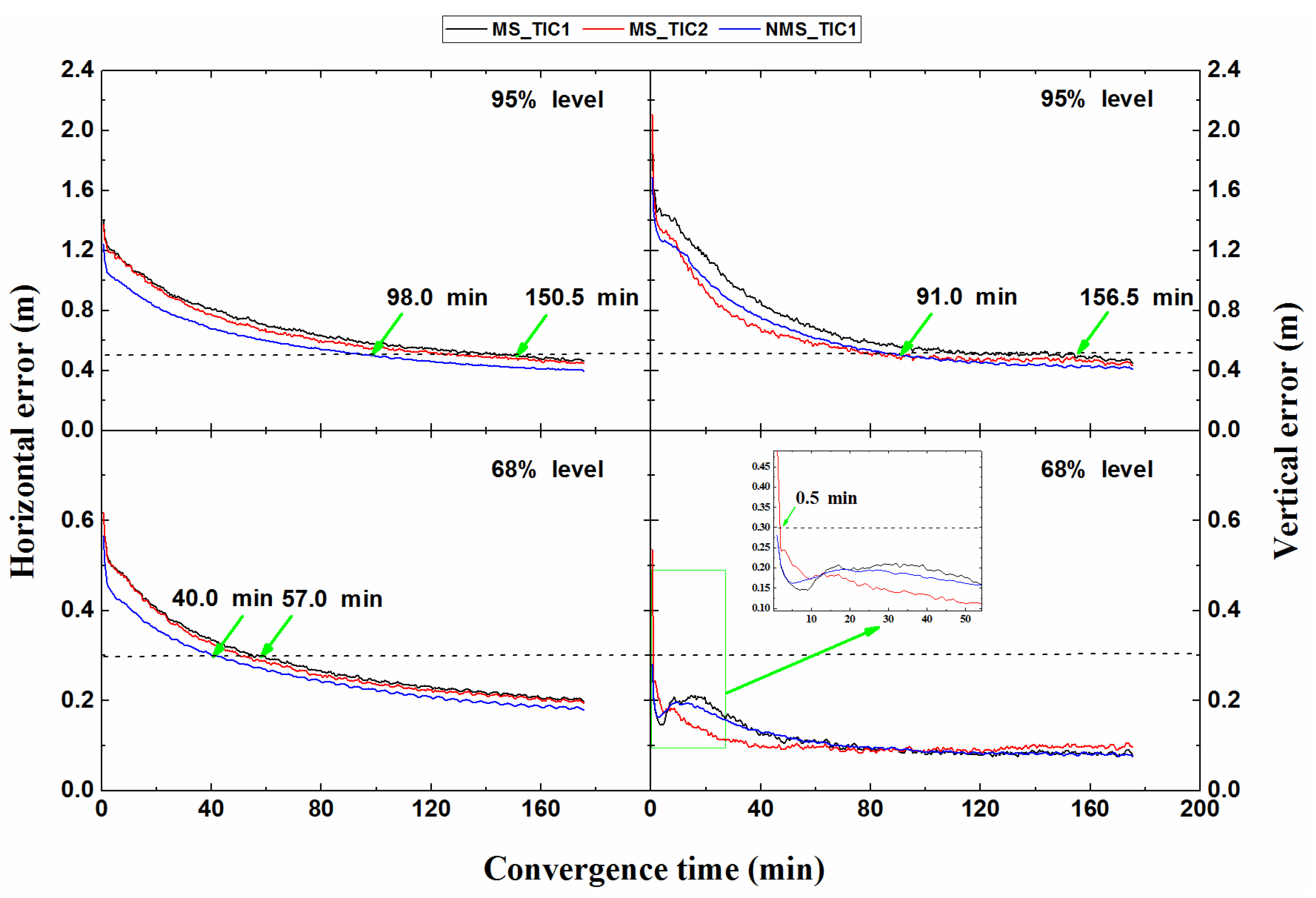
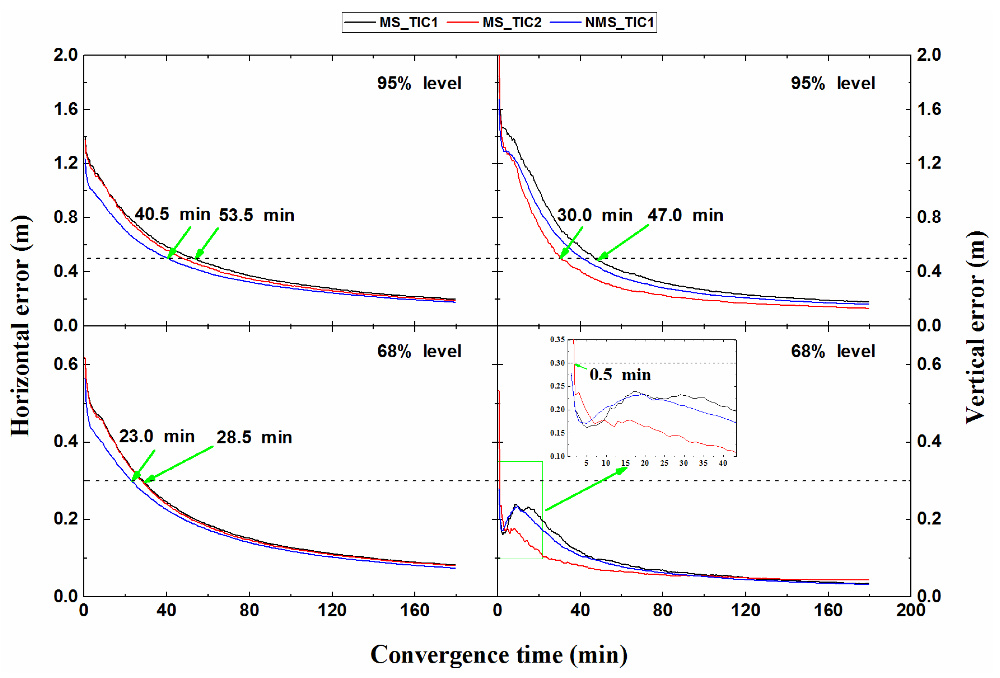
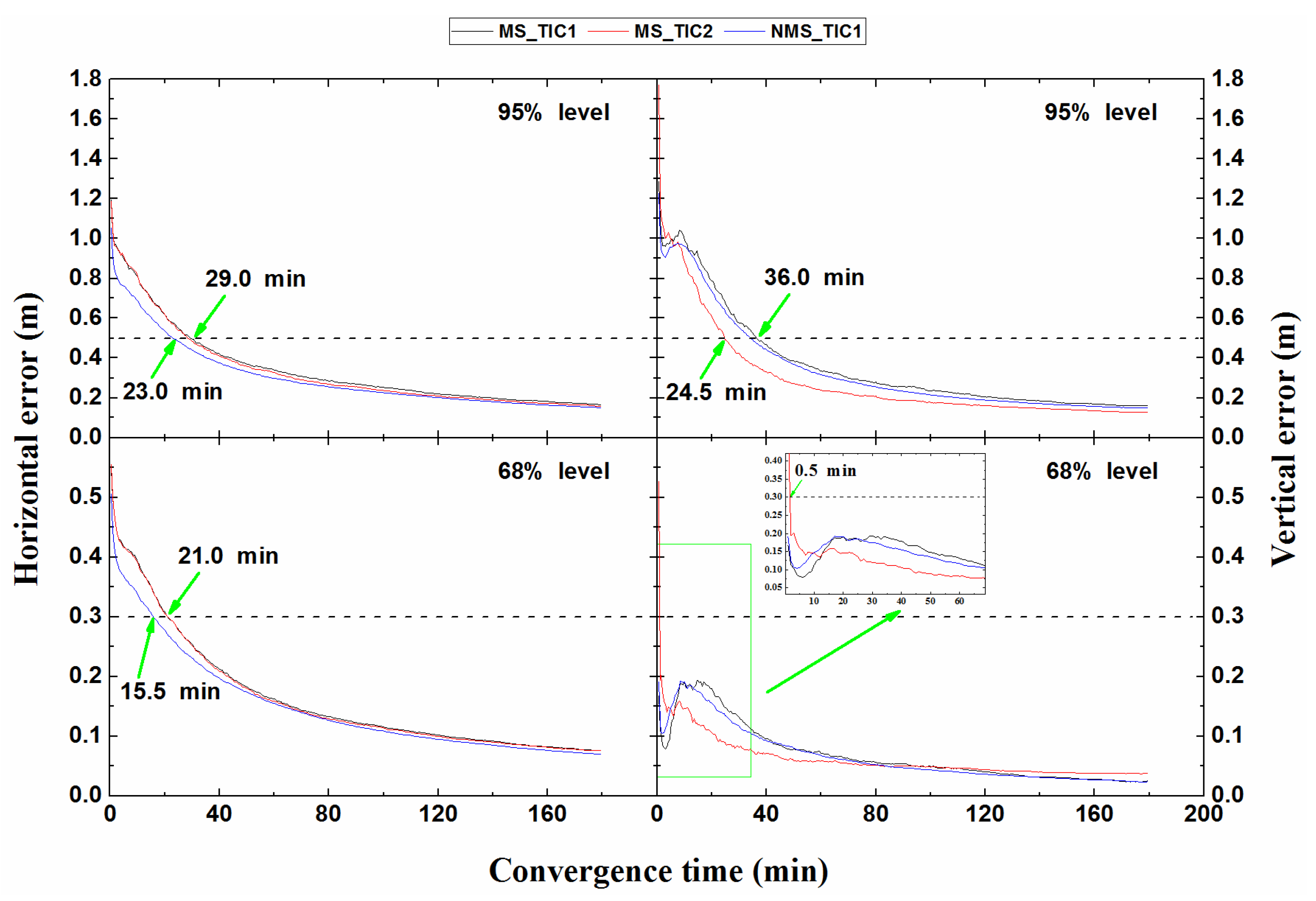
This section will analyze the convergence time and positioning accuracy of the stations in different MS periods and at low, middle, and high latitudes. The PPP performance in terms of convergence time in the horizontal and vertical components was evaluated at 68% and 95% levels. 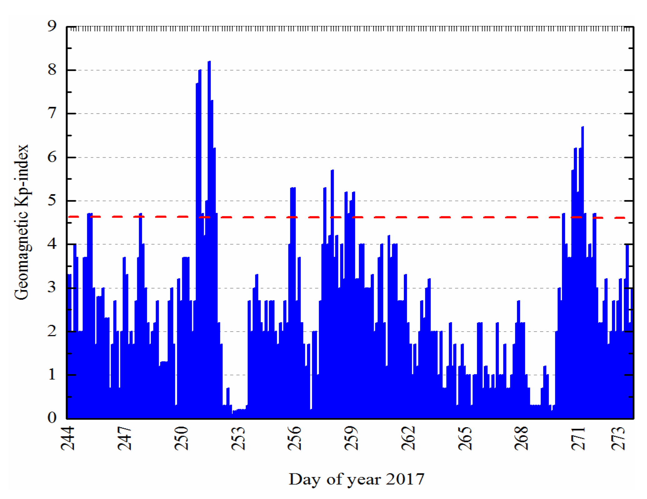For SF PPP solutions, when the positioning accuracy was better than 0.5 m (95%) and 0.3 m (68%) in the horizontal and vertical components, respectively, and was maintained at all the epochs, the solution was considered to be convergence [10]. We analyzed the effects of SF GPS convergence time on TIC1 and TIC2 schemes. We performed statistical analysis of the convergence times during the MS and NMS periods in two constraint schemes.

4.1. Different Magnetic Storm Results

This section analyzes the effects of SF PPP on convergence time and positioning accuracy during magnetic and non-magnetic storm periods, and under different constraints, as well as in static and dynamic modes.

It can be concluded from Figure 4 and Figure 5 that the convergence time in the vertical component was shorter than the horizontal component under the same environment and constraints, except for the kinematic positioning in the MS period and the static positioning in the NMS period of the TIC1 in the 95% level. In the MS period, when the tropospheric constraints were increased, the convergence time was reduced, except in the vertical component at the 68% level. The convergence time in the MS period was longer than the NMS period of the TIC1.

Table 2. The convergence times of GPS static and kinematic SF PPP in MS and NMS of TIC1 or TIC2.

Scheme	Kinematic SF PPP (min)				Static SF PPP (min)
	H (95%)	H (68%)	V (95%)	V (68%)	H (95%)	H (68%)	V (95%)	V (68%)
TIC1_MS	150.5	57.0	156.5	0.0	53.5	28.5	47.0	0.0
TIC2_MS	134.5	50.0	103.0	0.5	47.5	27.5	30.0	0.5
TIC1_NMS	98.0	40.0	91.0	0.0	40.5	23.0	41.0	0.0

shows that for the TIC2 at the 95% level, the convergence time in the kinematic mode was shortened by 10.6% in the horizontal component and 34.2% in the vertical component in the MS period when compared to the TIC1. In the static mode, the convergence time was improved from 53.5 to 47.5 min (11.2%) in the horizontal component and by 36.2% from 47.0 to 30.0 min in the vertical component. At the 68% level, the convergence time was shortened by 12.3% and 3.5% in the horizontal component of the TIC2 in the kinematic and static modes, respectively, which were comparable to the TIC1 in the MS period. However, the convergence time of TIC2 in the vertical component was 0.5 min longer than TIC1. The convergence time of TIC1 in the NMS period will be further analyzed. When compared to the MS period, the convergence time in the horizontal and vertical components was shortened by 34.9% and 41.8%, respectively, in the kinematic mode and at the 95% level in the NMS period. While in the static mode and at the 95% level, the convergence time was 24.3% and 12.8%, respectively. When compared to the MS period, in the horizontal component and at the 68% level, the TIC1 at the NMS period shortened the convergence time by 29.8% and 19.3% in the kinematic mode and static mode, respectively. However, their convergence time was equal to 0 in the vertical component.

In order to compare the final positioning accuracy in the case of the MS and NMS periods, the root mean square (RMS) error in the horizontal and vertical components as well as in the static and kinematic mode were estimated. The RMS error was based on the statistics of the last 15 min of the position solution error [17]. From

Table 3. The RMS of GPS static and kinematic SF PPP in MS and NMS of TIC1 or TIC2.

Scheme	Kinematic SF PPP (m)				Static SF PPP (m)
	H (95%)	H (68%)	V (95%)	V (68%)	H (95%)	H (68%)	V (95%)	V (68%)
TIC1_MS	0.475	0.204	0.474	0.083	0.205	0.085	0.182	0.035
TIC2_MS	0.457	0.200	0.452	0.098	0.195	0.083	0.135	0.043
TIC1_NMS	0.406	0.184	0.421	0.080	0.182	0.077	0.164	0.033

, it was overall concluded that TIC2 had a lower RMS compared to TIC1 during the MS period, except in the vertical component at the 68% level. The RMS value of TIC1 in the NMS period was smaller than that in the MS period.

4.2. Different Latitudes Area Results

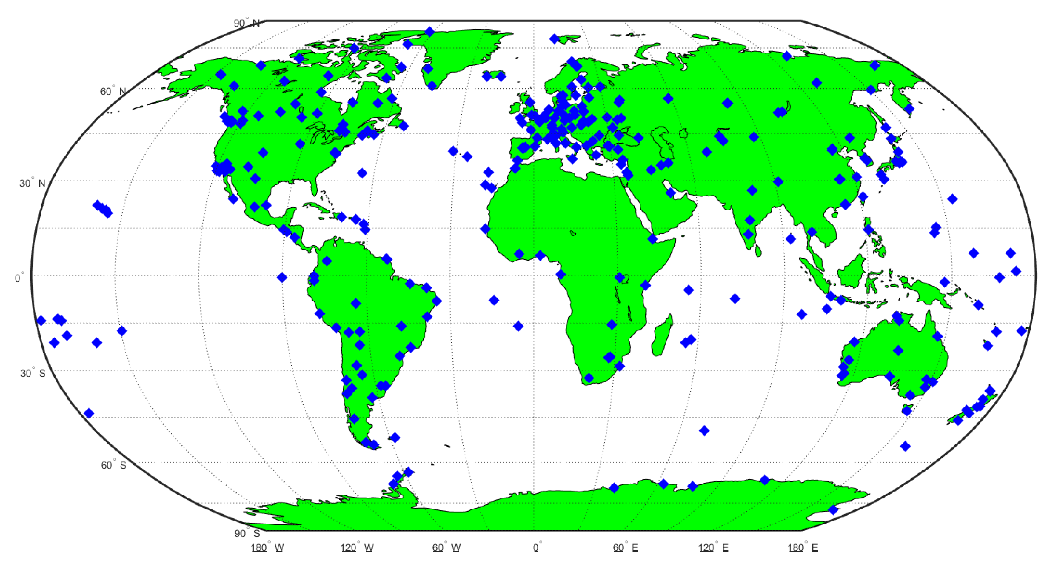
From the above analysis, it can be concluded that the advantage of TIC2 compared to TIC1 was not obvious in the MS period, so the whole number of GPS stations was divided into three latitudinal bands (high-latitude band, middle-latitude band, and low-latitude band). The TIC1 and TIC2 localization performance of SF PPP during MS and NMS periods were analyzed.

4.2.1. Low-Latitude Area Results

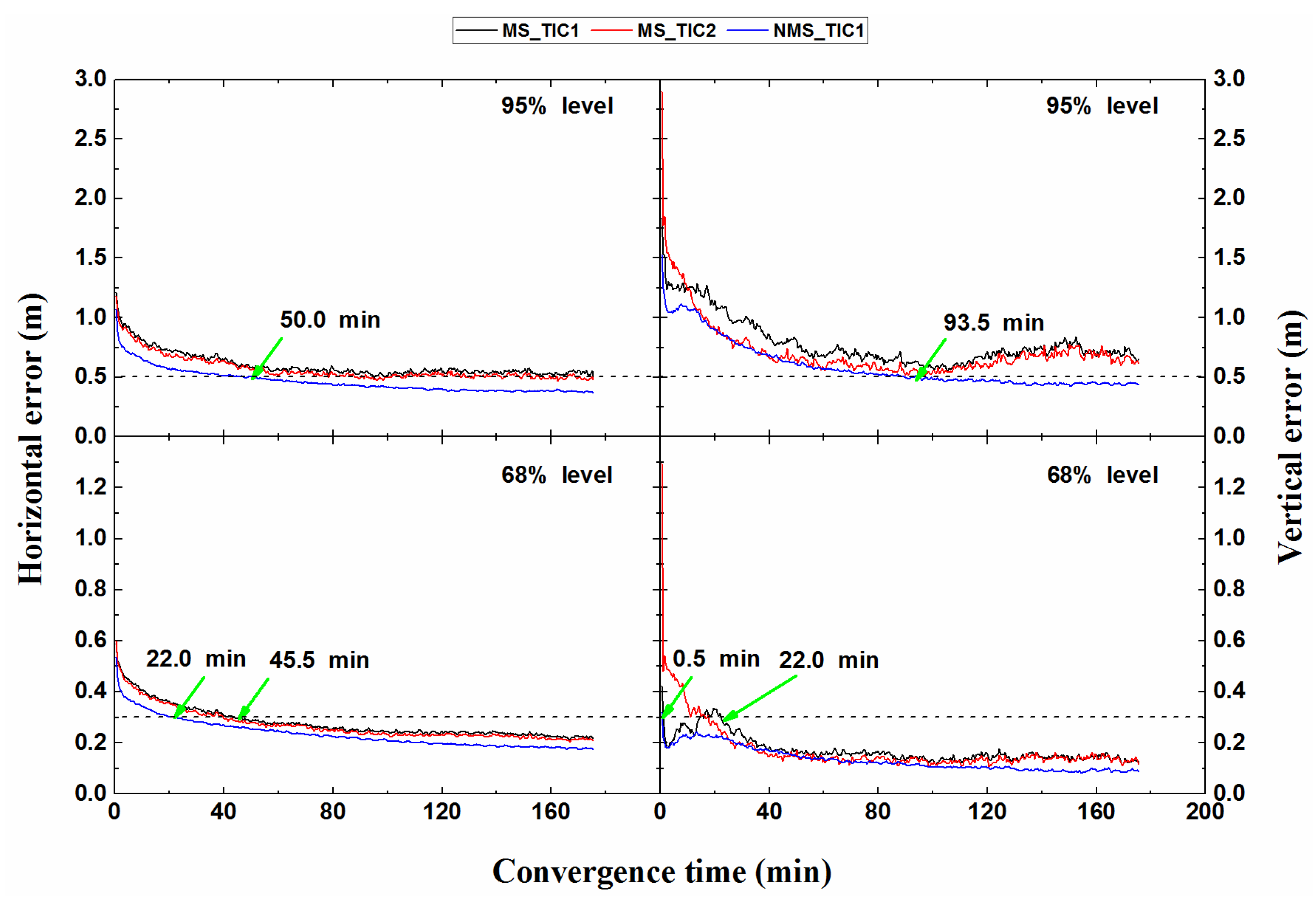
In order to verify the results from the low-latitude area, the positioning accuracy and convergence time of SF PPP in static and dynamic modes during MS and NMS periods were analyzed.

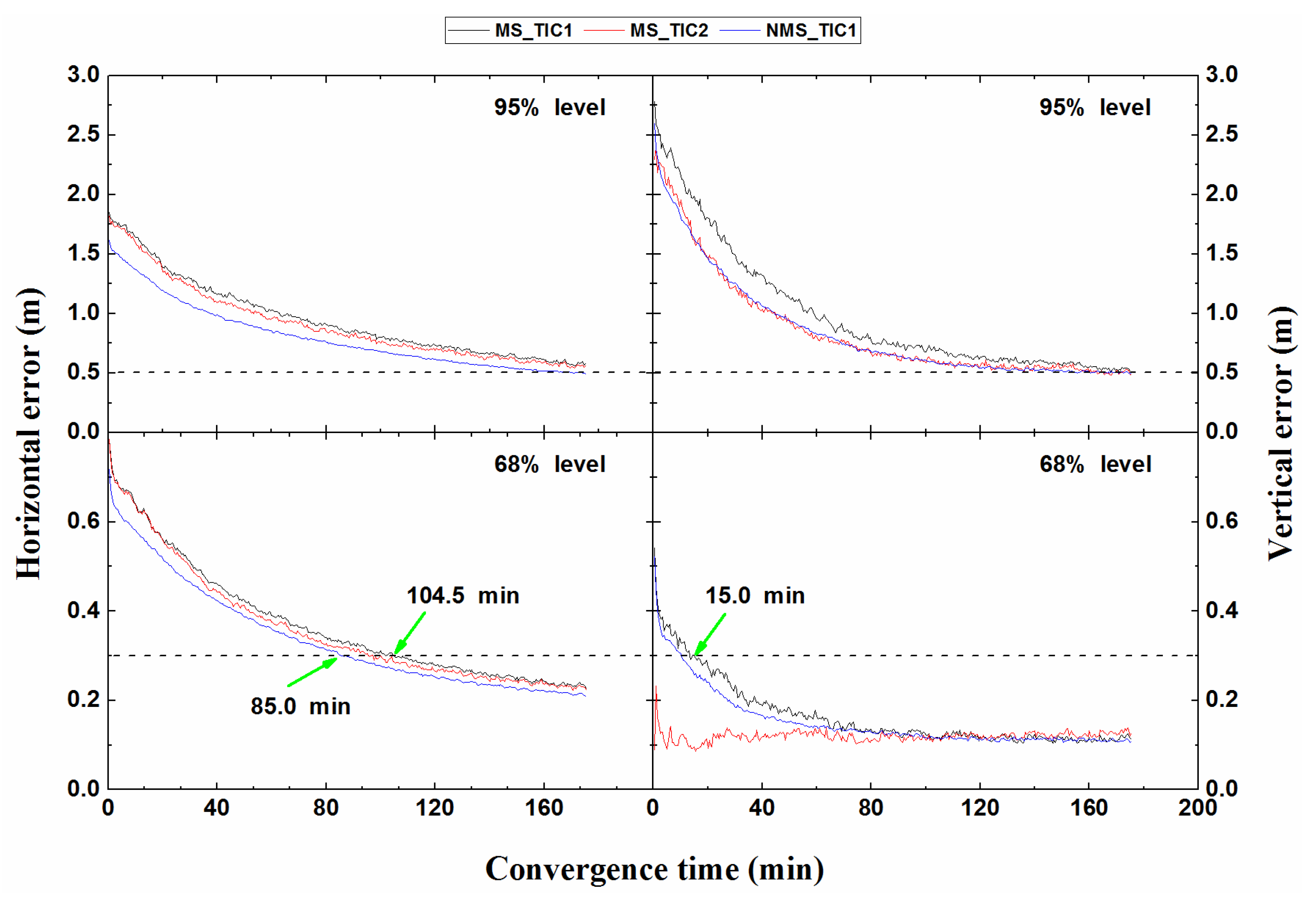
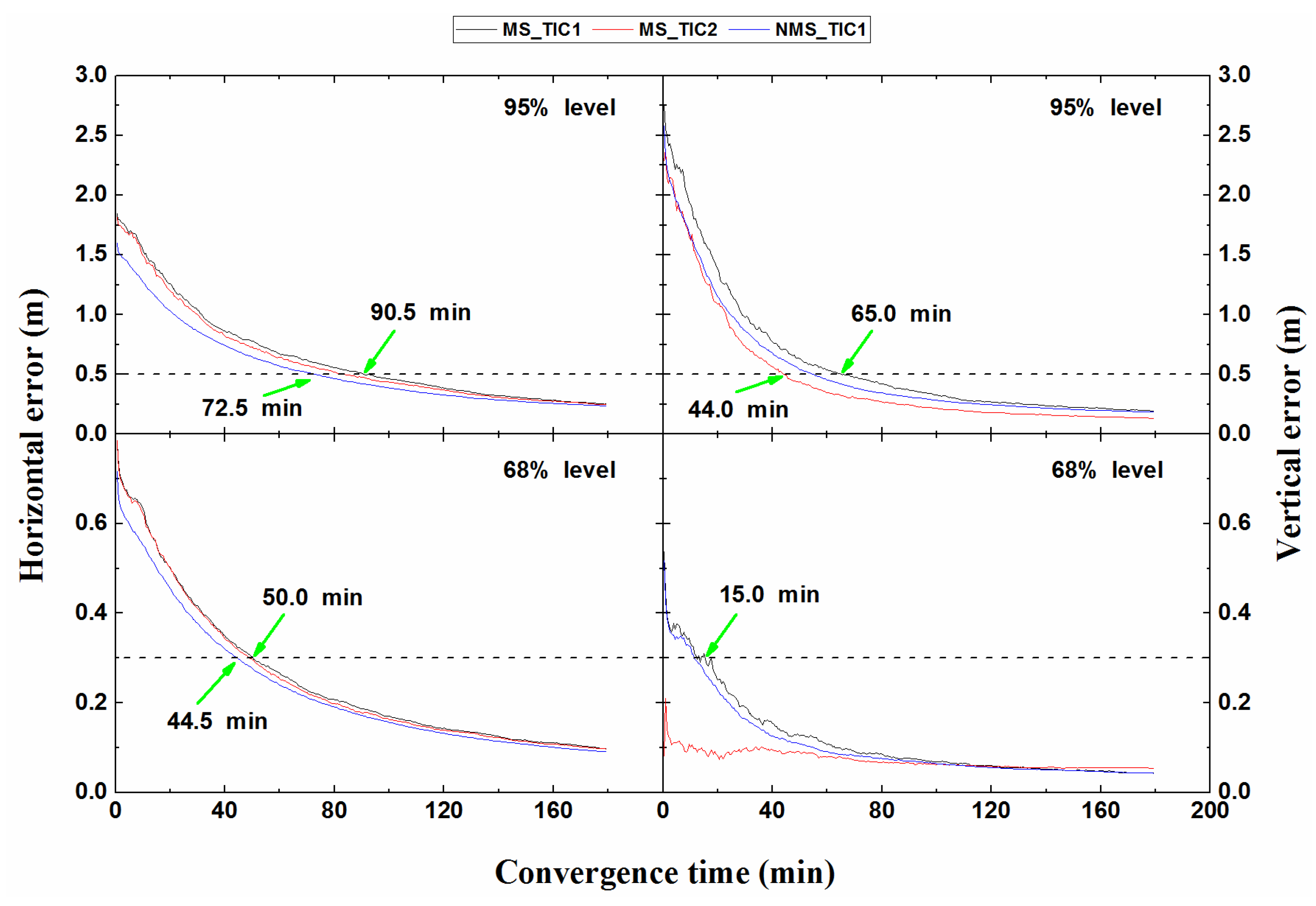
From Figure 6 in the kinematic mode, it can be seen that if the station was located in the low-latitude region, at the 95% level, TIC1 and TIC2 in the MS period and TIC1 in the NMS period did not converge. At the 68% level, the convergence time was longer than that of the stations distributed around the world. This may be due to fewer stations in the low-latitude area, which results in lower accuracy of the GIMs and the ZTD product, resulting in longer or no convergence time. In the static mode, although the convergence time was extended, it also converged, as shown in Figure 7.

From analysis in

Table 4. The convergence times of GPS static and kinematic SF PPP in MS and NMS of TIC1 or TIC2.

Scheme	Kinematic SF PPP (min)				Static SF PPP (min)
	H (95%)	H (68%)	V (95%)	V (68%)	H (95%)	H (68%)	V (95%)	V (68%)
TIC1_MS	--	104.5	--	15.0	90.5	50.0	65.0	15.0
TIC2_MS	--	97.0	--	0.0	83.0	48.5	44.0	0.0
TIC1_NMS	--	85.0	--	10.0	72.5	44.5	54.5	11.0

, it can be seen that in the low-latitude region, the convergence time of TIC2 in the vertical component was shorter than that of TIC1 in the MS period, and also shorter than the convergence time of TIC1 in the NMS period. This showed that the tropospheric constraints in the low-latitude region contributed more to the convergence time in the vertical component. After the tropospheric constraint was added, the positioning accuracy was instantaneously below the threshold level of 68%, thereby achieving the effect of the convergence time being 0 min. However, the horizontal component convergence time was still the shortest in the NMS period, which was at least 11.0% shorter than TIC1.

It was concluded in

Table 5. The RMS of GPS static and kinematic SF PPP in MS and NMS of TIC1 or TIC2.

Scheme	Kinematic SF PPP (m)				Static SF PPP (m)
	H (95%)	H (68%)	V (95%)	V (68%)	H (95%)	H (68%)	V (95%)	V (68%)
TIC1_MS	0.587	0.235	0.534	0.114	0.262	0.103	0.201	0.044
TIC2_MS	0.567	0.231	0.505	0.127	0.257	0.101	0.138	0.055
TIC1_NMS	0.508	0.216	0.505	0.110	0.243	0.094	0.189	0.044

that in the MS period of the low-latitude region, the RMS values of TIC2 and TIC1 were almost the same. For TIC1, the RMS value in the NMS period was smaller than that in the MS period, indicating that the MS had an influence on the positioning accuracy of the TIC1. The maximum RMS difference of TIC1 was 7.9 cm between the NMS period and the MS period. This result had a great influence on the positioning accuracy.

4.2.2. Middle-Latitude Area Results

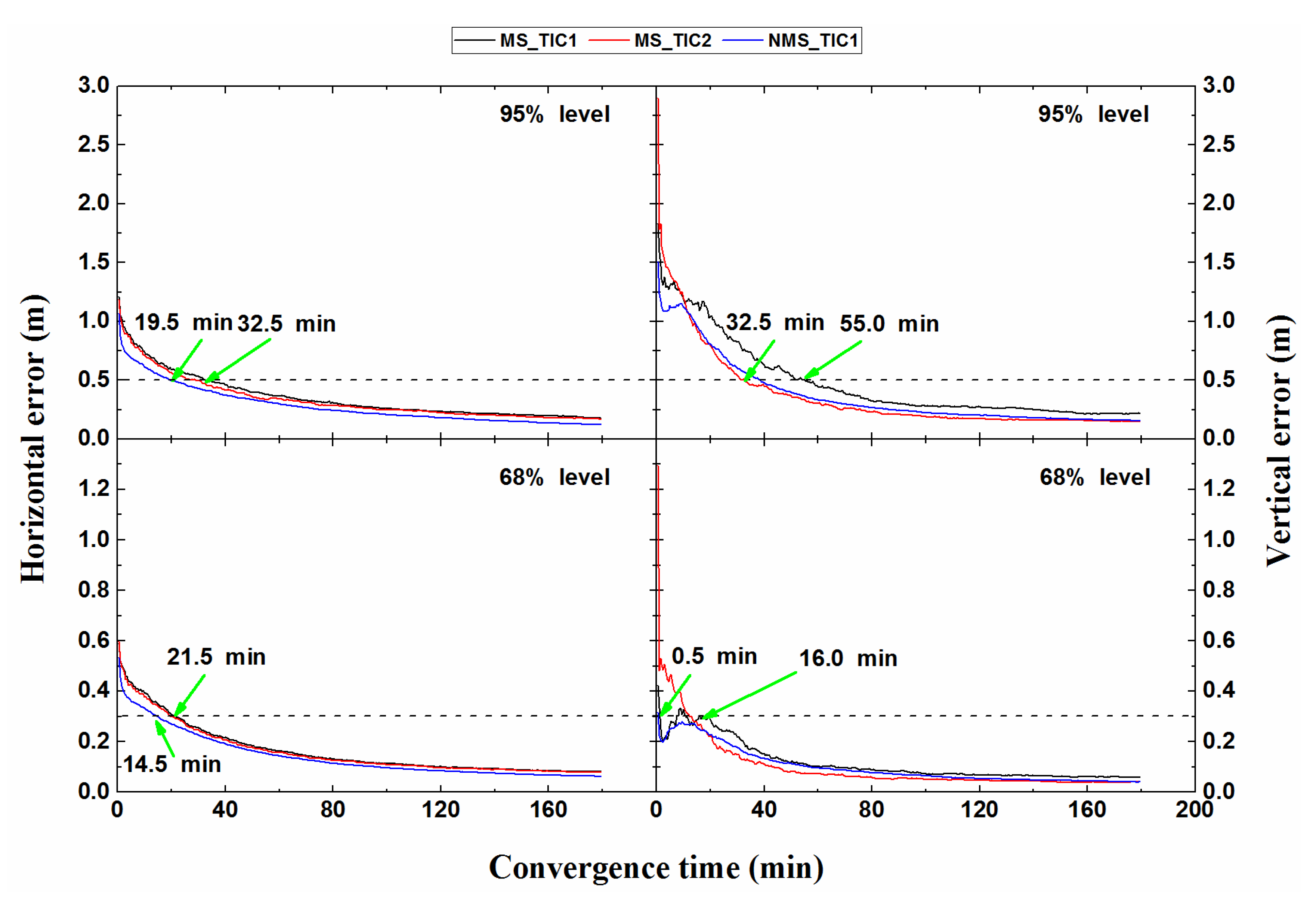
In order to verify the results for the middle-latitude area, the positioning accuracy and convergence time of SF PPP in static and dynamic modes during MS and NMS periods were analyzed.

It can be concluded from Figure 8, Figure 9, and

Table 6. The convergence times of GPS static and kinematic SF PPP in MS and NMS of TIC1 or TIC2.

Scheme	Kinematic SF PPP (min)				Static SF PPP (min)
	H (95%)	H (68%)	V (95%)	V (68%)	H (95%)	H (68%)	V (95%)	V (68%)
TIC1_MS	72.5	36.5	71.0	0.0	29.0	21.0	36.0	0.0
TIC2_MS	68.5	33.0	47.0	0.5	28.0	21.0	24.5	0.5
TIC1_NMS	43.0	23.5	64.5	0.0	23.0	15.5	34.0	0.0

that the convergence time of TIC1 in the NMS period was the shortest in the horizontal component. The convergence time of the TIC2 in the MS period was the shortest in the vertical component, except for at the 68% level, where it was slightly longer than the shortest convergence time, which was 0.5 minutes. At the 95% level, the TIC2 was comparable to the TIC1 in the MS period, and addition of tropospheric constraints reduced the convergence times by 5.5% (horizontal component) and 33.8% (vertical component) for the kinematic mode, and for the static mode they were reduced by 3.4% (horizontal component) and 31.9% (vertical component). At the 68% level, convergence time was reduced by 9.6% in the horizontal component in the kinematic mode. In the static mode, the convergence times were equal. However, at the 68% level, the convergence time of TIC2 was 0.5 min longer than the TIC1 in the vertical component. The results showed that TIC1 in the NMS period in the 68% and 95% level of kinematic and static modes accelerated the convergence. The convergence time improved by at least 5.6% compared to in the MS period. Of course, at the 68% level the convergence times were equal in the vertical component.

The laws in Table 6 and

Table 7. The RMS of GPS static and kinematic SF PPP in MS and NMS of TIC1 or TIC2.

Scheme	Kinematic SF PPP (m)				Static SF PPP (m)
	H (95%)	H (68%)	V (95%)	V (68%)	H (95%)	H (68%)	V (95%)	V (68%)
TIC1_MS	0.396	0.186	0.395	0.059	0.171	0.078	0.162	0.025
TIC2_MS	0.386	0.184	0.387	0.079	0.164	0.077	0.129	0.038
TIC1_NMS	0.354	0.172	0.371	0.064	0.156	0.072	0.151	0.025

are similar, except that the RMS values of TIC1 during the MS period and the NMS period became smaller. In the middle latitudes, influence of the ionosphere was moderate or low, which was comparable to the low-latitude region, so the difference in positioning results was small in both environments.

4.2.3. High-Latitude Area Results

In order to verify the results for the high-latitude area, the positioning accuracy and convergence time of SF PPP in static and dynamic modes during MS and NMS periods were analyzed.

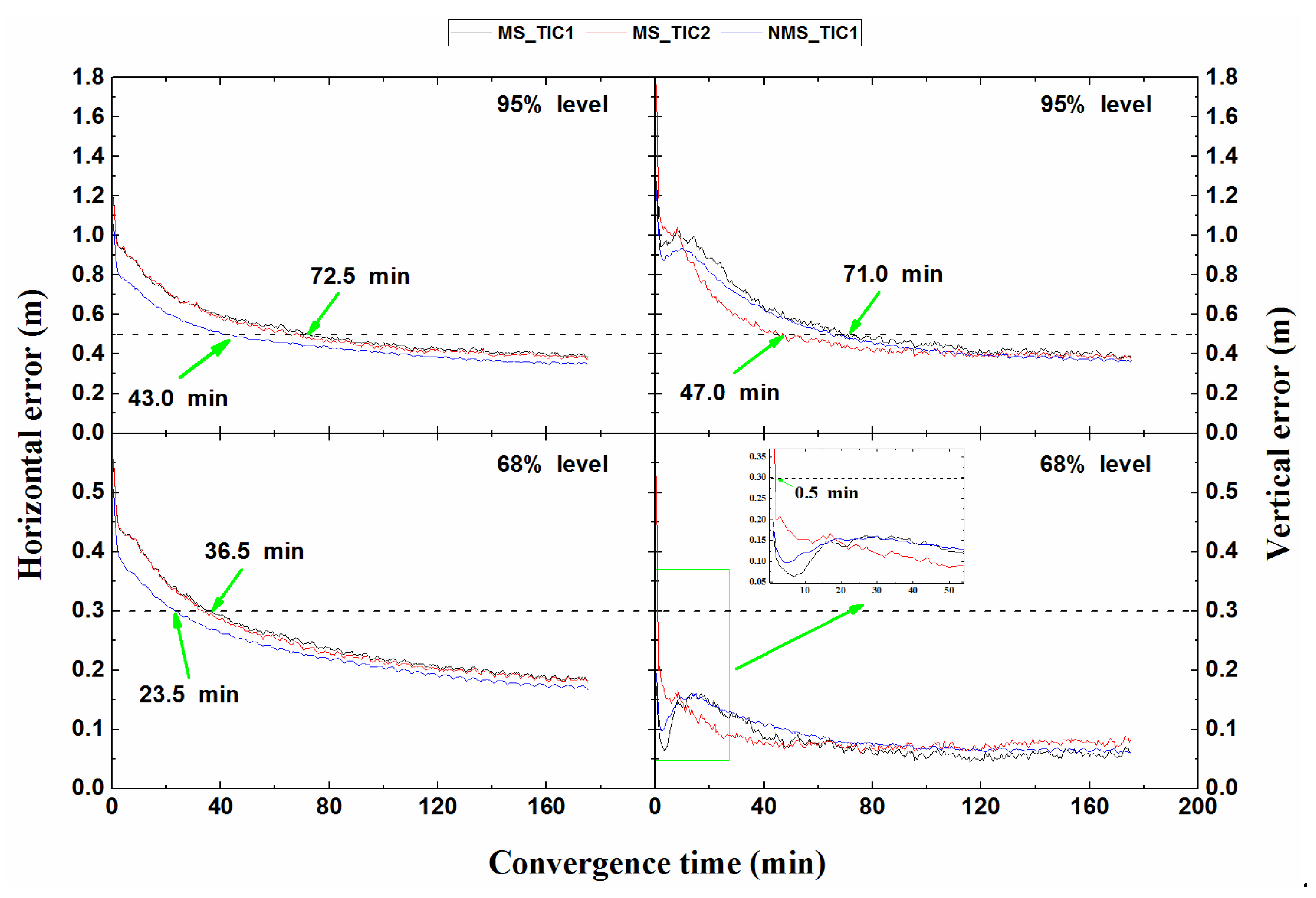
It was concluded in Figure 10 that at the 95% level, TIC1 and TIC2 still did not converge in the kinematic mode in the MS period, but TIC1 converged in the NMS period. Although the number of stations distributed in the high latitude band was less than the low latitude band, TIC1 converged in the NMS period, indicating that the occurrence of magnetic storms had a greater impact on the convergence time of SF PPP. The effect of the magnetic storms on the convergence time was also demonstrated in Figure 11, and the convergence time of TIC1 in the NMS period was shorter than that of TIC2 during the MS period in the static mode. As shown in

Table 8. The convergence times of GPS static and kinematic SF PPP in MS and NMS of TIC1 or TIC2.

Scheme	Kinematic SF PPP (min)				Static SF PPP (min)
	H (95%)	H (68%)	V (95%)	V (68%)	H (95%)	H (68%)	V (95%)	V (68%)
TIC1_MS	--	45.5	--	22.0	32.5	21.5	55.0	16.0
TIC2_MS	--	39.5	--	17.5	29.0	19.5	32.5	13.0
TIC1_NMS	50.0	22.0	93.5	0.5	19.5	14.5	38.5	0.5

, adding tropospheric constraints shortened the convergence time of TIC2 in the MS period by 13.2% and 20.4% in the horizontal and vertical components, respectively, in the kinematic mode and at the 68% level which was comparable to TIC1. Compared to TIC1 the percentage of convergence time in the static mode was shorted to 10.8%, 9.3%, 40.9%, and 18.8% at the 95% level and horizontal component, the 68% level and horizontal component, the 95% level and vertical component, and at the 68% level and vertical component, respectively. Up to 51.6% and 97.7% reduction occurred in the horizontal and vertical components, respectively, in the kinematic mode and at the 68% level, which for TIC1 in the NMS period was comparable to the MS period. The TIC1 in the static mode, which in the NMS period was comparable to the MS period, had a shorter convergence time at the 95% level and horizontal component, the 68% level and horizontal component, the 95% level and vertical component, and at the 68% level and vertical component, which shortened times 40.0%, 32.6%, 30.0%, and 96.9%, respectively.

It can be seen from

Table 9. The RMS of GPS static and kinematic SF PPP in MS and NMS of TIC1 or TIC2.

Scheme	Kinematic SF PPP (m)				Static SF PPP (m)
	H (95%)	H (68%)	V (95%)	V (68%)	H (95%)	H (68%)	V (95%)	V (68%)
TIC1_MS	0.535	0.223	0.702	0.138	0.186	0.082	0.215	0.060
TIC2_MS	0.495	0.214	0.659	0.136	0.175	0.079	0.151	0.040
TIC1_NMS	0.380	0.179	0.444	0.091	0.127	0.064	0.159	0.042

that during the MS period, the RMS value of TIC2 was smaller than that of TIC1. Under TIC1, the RMS value of the MS period was greater than that of the NMS period. This showed that in the high latitude region, not do only the tropospheric constraints have an influence on the convergence time, but they also affect the positioning accuracy.

5. Conclusions

This paper studies the effects of TIC1 and TIC2 on the convergence time and positioning accuracy in SF PPP, and analyzes its positioning performance during MS and NMS periods. By comparing the positioning performance in low, middle, and high latitude areas, the following conclusions are drawn:

(1) Through statistical analysis of the SF PPP convergence time and positioning accuracy of the globally distributed stations, it was found that during the MS period, the TIC2 convergence time was shorter than TIC1 as a whole, with a minimum improvement of 3.9%. For TIC1, the convergence time in the MS period was longer than in the NMS period, and the maximum convergence time could be extended by 41.8%.

(2) The stations distributed around the world were further subdivided into high latitude, mid-latitude, and low latitude areas. According to our statistical analysis, the influence of ionospheric disturbances was large at low latitudes, resulting in a convergence time increase. The effect of increasing tropospheric constraints was not as good as TIC1 in the NMS period. Since at high latitudes the influence of the ionosphere was moderate or low, the overall convergence time was shorter than in the low latitude regions. However, the number of stations in the high latitude area was only 20% of that in the mid-latitude area; therefore the accuracy of the GIMs and the ZTD products was slightly lower and the convergence time was longer than the mid-latitude area under the TIC1 and TIC2. During the MS period, it was shown that the convergence times for the TIC2 cases became shorter by about 1.5 min, 0 min, and 2 min for the low, middle, and high latitude areas, respectively, in comparison with the TIC1. For TIC1 in the NMS period compared to in the MS period the convergence times were shortened by at least 4 min, 0 min, and 7 min, respectively. Some mode convergence times were not shortened in the mid-latitude, and this was because the ionospheric activity in the mid-latitude region was less than that in the low-latitude region, and there were more stations, so the precision of the GIMs and ZTD products were also slightly higher.

(3) On the whole, TIC1 and TIC2 had little effect on the final positioning accuracy in the MS period, and the overall maximum difference was not more than 2 cm. The positioning accuracy of TIC1 in the NMS period was improved, compared to the MS period, by at least 2 cm, except at the 68% level in the vertical direction.