Out-of-Plane Bending of Functionally Graded Thin Plates with a Circular Hole

Abstract

The out-of-plane bending problems of functionally graded thin plates with a circular hole are studied for two-dimensional deformations. The thin plates have arbitrary variations of elastic properties along the radial direction. The general solutions of the stresses and moments are presented for the plates subjected to remote bending moments based on the theory of complex variable functions. Two different cases—a whole functionally graded plate with a circular hole and a functionally graded ring reinforced in a homogeneous perforated plate—are considered by numerical examples. The influence of parameters like Young’s modulus and Poisson’s ratio, function types of these elastic properties, and width of the reinforcing ring on the moments around the hole is presented. It is shown that the moment concentration, caused by the geometric discontinuity of the hole in the traditional homogeneous plate, can be well relieved or even eliminated by careful selection of the above parameters. The results for some special cases are compared with previous literatures and are found in good agreement.

1. Introduction

Holes exist widely in engineering structures for either design or manufacture reasons, and the high stress concentration around them has been a serious issue to the engineers and designers for many years. In order to achieve better machine designs, some classical references such as Norton [1], Budynas et al. [2,3], and Pilkey and Pilkey [4] summarized and provided various important solutions of stress concentration factor (SCF) in engineering structures. The effects of stress concentration on the fatigue strength and life of structures are of great importance, especially when the structures are designed to carry high loads [5,6,7]. Therefore, it has been of great concern to reduce the stress concentration near holes during the structure design and safety maintenance in engineering. Recent research [8,9,10,11] indicates that the stress concentration around the holes can be effectively reduced by introducing a reinforcing ring made by functionally graded material (FGM).

FGM is an advanced composite material in which the material elements (composition and structure) change continuously along one or more directions. The continuous elements in FGM can successfully avoid the mismatch of the material properties at the interface [12]. The introduction of the FGM reinforcing ring with radially varying material properties can not only reduce the stress concentration around the hole, but also enhance the connection strength at the interface [13,14]. Therefore, many studies have been carried out on the analysis of stresses around holes in FGM in the past 20 years.

Inspired by the excellent material distributions near the natural holes in a load-bearing bone, Huang et al. [15,16] first studied and improved the strength and loading capacity of a plate with a circular hole by controlling the radially varying Young’s modulus in the plate. The optimization designs were carried out on choosing the proper mathematical functions of the axisymmetric Young’s modulus for increased strength. The stress concentrations in an FGM plate with a center circular hole or elliptical hole were numerically analyzed by Kubair and Bhanu-Chandar [17] and Wang et al. [18], respectively, based on the finite element method. They both considered the variations of Young’s modulus along three different directions: radial direction, x direction, and Y direction. By means of the complex variable methods, Yang et al. [19,20] presented the semi-analytical solutions of the stress fields in the infinite and finite FGM plates containing a circular hole under arbitrary in-plane constant loads. For some specific radial varying functions of Young’s modulus, Mohammadi et al. [21] obtained the analytical solution of stresses in an FGM plate with a circular hole under uniform tension. Goyat et al. [22] analyzed the effects of different radial variations of Young’s modulus on the stress concentration factor (SCF) around the hole in FGM plate with the method of extended finite element. Considering the cost and difficulty of material preparation, Sburlati [23] proposed a more feasible method to reduce the stress concentration by inserting a thin FGM ring around the hole. The analytical solution of the stress fields is presented for the plate subjected to far-field uniaxial tension, and the effects of the homogeneous ring and FGM ring on the SCF are compared by numerical examples. Recently, Nie et al. [24] derived the analytical SCF in an FGM plate with a circular hole as Young’s modulus and Poisson’s ratio change along the radial direction with exponential function or power function, and they laid emphasis on the tailoring problem of the material. Their results show that the desired SCF can be obtained by tailoring the radial variation of Young’s modulus, and at the same time, the hoop stress is almost uniformly distributed in the whole plate.

The previous works cited above primarily focus on the case of an FGM plate subjected to in-plane loading in the middle surface of the plate, and not much work can be found for the analysis of the case of out-of-plane loads. Kubair [25,26] studied the SCF and stress-gradients due to a circular hole in a radial FGM plate subjected to anti-plane shear loading and obtained the closed expressions for the stresses and displacements. A novel definition is introduced for the SCF in FGM plates with geometrical discontinuities in general. Shi [27] presented an analytical solution of the elastic stress fields around a circular elastic inclusion in a radial FGM plate under a uniform anti-plane shear loading at infinity. Guan and Li [28] analyzed the stress concentration around an arbitrarily shaped hole reinforced with an FGM layer in an infinite plate under anti-plane shear and performed the optimized analysis of the SCF. The above works are mainly for anti-plane problems. In fact, in addition to anti-plane shear loading, structures subjected to out-of-plane bending moments are also very common in engineering. Thus, it is also very significant to study the bending problems of FGM plates.

Recently, some works have been made on the out-of-plane bending of FGM plates through thickness material property variation. For example, Yang et al. [29,30] investigated the resultant force concentration around holes in a transversely isotropic FGM plate with the material properties varying along the thickness direction under concentrated loads and moments. Dave and Sharma [31] provided a solution of stresses and moments around circular and elliptical holes in FGM infinite plates with material property variation along the thickness using a complex variable approach. However, to the best of the author’s knowledge, the bending of FGM plates with radially varying material properties has not yet been addressed.

In this paper, the bending stress concentration around a circular hole in an FGM thin plate, which has arbitrary variations of elastic properties along the radial direction, is investigated based on the theory of complex variable functions. Following the introduction, the general solutions of the stresses and moments are presented for the plate subjected to out-of-plane bending moments by means of the method of piece-wise homogeneous layers. Then, numerical examples are given to discuss the effect of different radial variations of elastic parameters on the distribution of the moments for two different cases: a whole FGM plate with a circular hole and an FGM ring reinforced in a homogeneous perforated plate. Finally, conclusions of the present work are summarized.

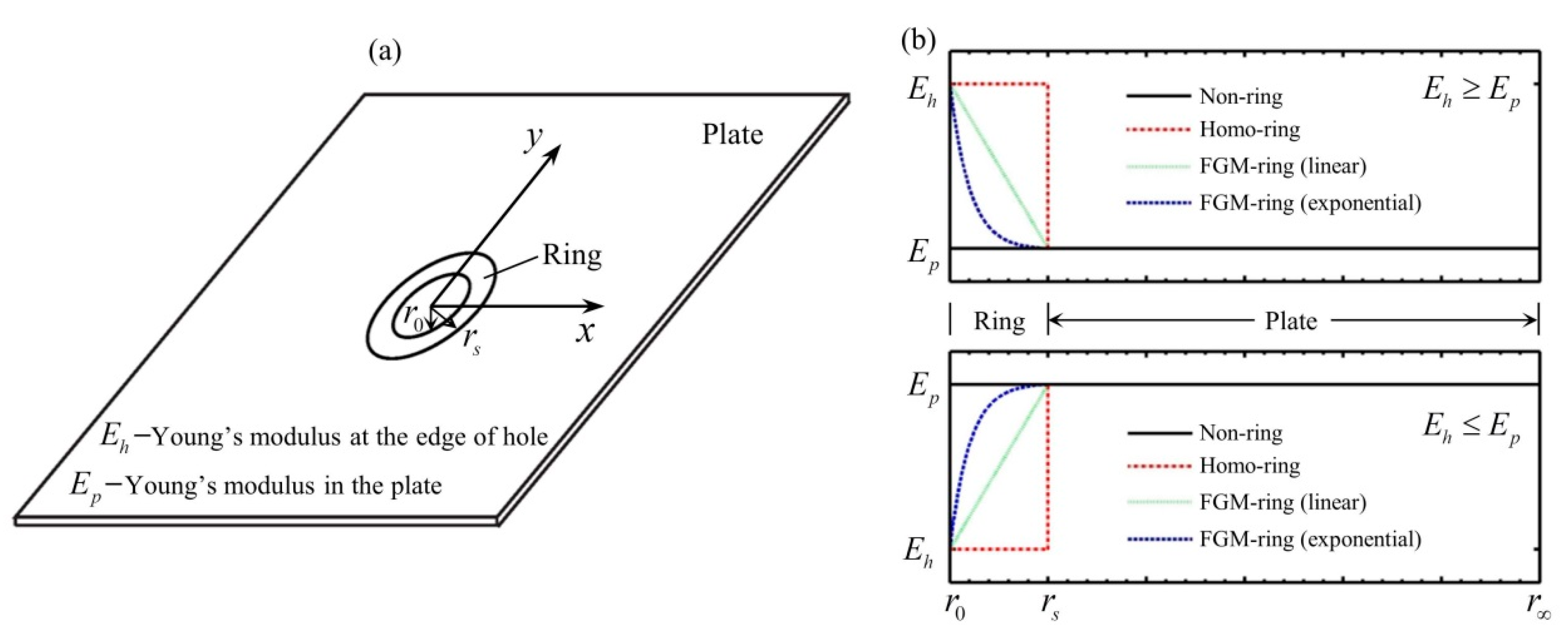
2. Problem Formulations

A functionally graded thin plate with a circular hole is deflected under remote bending moments $M_x$ and $M_y$ applied per unit length of the plate, as shown in Figure 1. The radius of the hole $r_0$ is taken to be small in comparison with the length of the sides and sufficiently large compared to the thickness of the plate $h$. The Young’s modulus $E$ and Poisson’s ratio $\nu$ change continuously along the radial direction with arbitrary function forms.

It is very hard to solve the problem by the analytical method due to the continuous and arbitrary changes of elastic parameters; hence, a semi-analytical method that is the piece-wise homogeneous layers is used here. The FGM plate is approximately divided into a homogenous plate containing a series of homogeneous concentric rings with equal width. As long as the number of rings is taken to be large enough, the elastic parameters in each ring could be regarded as unchanged. In this case, the problem can be solved by means of Muskhelishvili’s complex variable methods. The number of concentric rings is assumed as $s$, and their located domains are symbolized by $K_1$, $K_2$, …, $K_s$. $K_{s+1}$ is taken to represent the domain of the outer homogenous plate. The inner and outer radii of each circular ring $K_j\left(j=1,2,\cdots s\right)$ are denoted by $r_{j-1}$ and $r_j$, respectively.

3. General Solutions

For convenience, we introduce a cylindrical coordinate $(r,\theta )$ in the plane $xoy$ with the application of the hole center as the pole, the x-axis and $\theta$ as the polar axis and polar angle, respectively. The moments and transverse shear forces in the cylindrical coordinate can be expressed with two complex potential functions, $\phi (z)$ and $\psi (z)$, by formulas [32] (1) and (2):

$$M_{\theta }-M_r+2i{H}_{r\theta }=2D(1-v)e^{2i\theta }\left[\overline{z}{\phi }^{″}\left(z\right)+{\psi }^{″}\left(z\right)\right],$$

(1)

$$M_{\theta }+M_r=-4D(1+v)\mathrm{Re}\left[{\phi }^{\prime }\left(z\right)\right],$$

(2)

where $M_{\theta }$, $M_r$, and $H_{r\theta }$ are the bending moments and twisting moments, respectively, and the bending rigidity of the plate $D=E{h}^2/\left[12\left(1-{\nu }^2\right)\right]$.

The complex potential functions $\phi (z)$ and $\psi (z)$ can be determined by the following boundary conditions when the components of force $f_1$, $f_2$, components of displacement $u$, $v$ and deflection $w$ are given

$$D\left\{\left(1-v\right)\left[\overline{z}{{\phi }^{\prime }}_{}\left(z\right)+\psi \left(z\right)\right]-\left(3+v\right)\overline{\phi \left(z\right)}\right\}=f_1-i{f}_2,$$

(3)

$$\psi \left(z\right)+\overline{z}{{\phi }^{\prime }}_{}\left(z\right)+\overline{\phi \left(z\right)}=u-iv,$$

(4)

$$\mathrm{Re}\left[\chi \left(z\right)+\overline{z}\phi \left(z\right)\right]=w\left(x,y\right).$$

(5)

Here, $\chi \left(z\right)$ is a new complex potential function defined as $\chi \left(z\right)={\displaystyle \int \psi \left(z\right)dz}$. $f_1$ and $f_2$ are dependent on the bending moments and forces applied per unit length at the boundary

$$f_1-i{f}_2=-R{\displaystyle {\int }_0^{\theta }\left[im\left(\theta \right)+R{\displaystyle {\int }_0^{\theta }p\left(\theta \right)d\theta }\right]e^{-i\theta }}d\theta .$$

(6)

In the domain of the plate $K_{s+1}$, the complex potential functions ${\phi }_{s+1}\left(z\right)$ and ${\chi }_{s+1}\left(z\right)$ can be expressed in the following manner [32]:

$${\chi }_{s+1}\left(z\right)=R\left[{\displaystyle \sum _{k=0}^{\infty }{A}_k\frac{z^k}{R^k}}+\alpha \ln z+{\displaystyle \sum _{k=1}^{\infty }{\alpha }_{-k}\frac{R^k}{z^k}}\right],$$

(7)

$${\phi }_{s+1}\left(z\right)={\displaystyle \sum _{k=1}^{\infty }{B}_k\frac{z^k}{R^k}}+{\displaystyle \sum _{k=0}^{\infty }{\beta }_{-k}\frac{R^k}{z^k},}$$

(8)

where $\alpha$, ${\alpha }_{-k}$, ${\beta }_{-k}$ $\left(k=1,2,\cdots ,m+1\right)$ are unknown coefficients while $A_k$, $B_k$ are known coefficients dependent on the applied bending moments $M_x$ and $M_y$ at infinity; $R$ is the reference radius.

The complex potential functions ${\phi }_j\left(z\right)$ and ${\chi }_j\left(z\right)$ in each ring $K_j\left(j=1,2,\cdots ,s\right)$ can be expressed in the following manner [32]:

$${\chi }_j\left(z\right)=R\left[a^{(j)}\ln z+{\displaystyle \sum _{-\infty }^{+\infty }{a}_{{}_k}^{(j)}\frac{z^k}{R^k}}\right],$$

(9)

$${\phi }_j\left(z\right)={\displaystyle \sum _{-\infty }^{+\infty }{b}_{{}_k}^{(j)}\frac{z^k}{R^k},}$$

(10)

where $a^{(j)}$, $a_k^{(j)}$, $b_k^{(j)}$ $\left(k=1,2,\cdots ,m+1\right)$ are unknown coefficients.

Since there is no load at the edge of the hole, it is easy to get $f_1-i{f}_2=0$ in Equation (6). According to Equation (3), the equation of boundary condition at the edge of the hole $r=r_0$ will be written as

$$D_1\left\{\left(1-v_1\right)\left[\overline{z}{{\phi }^{\prime }}_1\left(z\right)+{\psi }_1\left(z\right)\right]-\left(3+v_1\right)\overline{{\phi }_1\left(z\right)}\right\}=0.$$

(11)

Substituting Equations (9) and (10) with $j=1$ and $z=r_0{e}^{i\theta }$ into Equation (11), and instead of $n_0=r_0/R$, we obtain the following equation after simplifications

$$D_1\cdot \{\left(1-v_1\right)\left[a^{\left(1\right)}{e}^{-i\theta }{n}_0^{-1}+{\displaystyle \sum _{k=-\infty }^{+\infty }{a}_k^{\left(1\right)}k{e}^{i\left(k-1\right)\theta }{n}_0^{k-1}+}{\displaystyle \sum _{k=-\infty }^{+\infty }{b}_k^{\left(1\right)}k{e}^{i\left(k-2\right)\theta }{n}_0^k}\right]-\left(3+v_1\right){\displaystyle \sum _{k=-\infty }^{+\infty }\overline{b_k^{\left(1\right)}}{e}^{-ik\theta }{n}_0^k}\}=0.$$

(12)

By comparing the coefficients of the same power of −2, −1, 0 $k$ and $-k$ of $e^{i\theta }$ in Equation (12), we can get a set of $2m+3$ linear equations listed as Equations (A1)–(A5) in Appendix A.

On the other hand, forces, displacements, and deflections satisfy the continuous conditions at the interface $r=r_j\left(j=1,2,\cdots ,s-1\right)$ between each adjacent rings $K_j$ and $K_{j+1}$. Hence, the equations of continuous condition can be written as follows on the basis of Equations (3)–(5)

$$D_j\left\{\left(1-v_j\right)\left[\overline{z}{{\phi }^{\prime }}_j\left(z\right)+{\psi }_j\left(z\right)\right]-\left(3+v_j\right)\overline{{\phi }_j\left(z\right)}\right\}$$

$$=D_{j+1}\left\{\left(1-v_{j+1}\right)\left[\overline{z}{{\phi }^{\prime }}_{j+1}\left(z\right)+{\psi }_{j+1}\left(z\right)\right]-\left(3+v_{j+1}\right)\overline{{\phi }_{j+1}\left(z\right)}\right\},$$

(13)

$${\psi }_j\left(z\right)+\overline{z}{{\phi }^{\prime }}_j\left(z\right)+\overline{{\phi }_j\left(z\right)}={\psi }_{j+1}\left(z\right)+\overline{z}{{\phi }^{\prime }}_{j+1}\left(z\right)+\overline{{\phi }_{j+1}\left(z\right)},$$

(14)

$$\mathrm{Re}\left[{\chi }_j\left(z\right)+\overline{z}{\phi }_j\left(z\right)\right]=\mathrm{Re}\left[{\chi }_{j+1}\left(z\right)+\overline{z}{\phi }_{j+1}\left(z\right)\right].$$

(15)

Introducing Equations (9) and (10) with $j=1,2,\cdots ,s-1$ and $z=r_j{e}^{i\theta }$ into Equations (13)–(15), and instead of $n_j=r_j/R$, we obtain the following lengthy equations after a series of somewhat arduous simplifications

$$D_j\cdot \{\left(1-v_j\right)[a^{\left(j\right)}{e}^{-i\theta }{n}_j^{-1}+{\displaystyle \sum _{k=2}^{+\infty }{a}_{-\left(k-1\right)}^{\left(j\right)}\left(1-k\right)e^{-ik\theta }{n}_j^{-k}}+{\displaystyle \sum _{k=0}^{+\infty }{a}_{k+1}^{\left(j\right)}\left(k+1\right)e^{ik\theta }{n}_j^k}$$

$$+{\displaystyle \sum _{k=3}^{+\infty }{b}_{-\left(k-2\right)}^{\left(j\right)}\left(2-k\right)e^{-ik\theta }{n}_j^{-\left(k-2\right)}+{\displaystyle \sum _{k=-1}^{+\infty }{b}_{k+2}^{\left(j\right)}\left(k+2\right)e^{ik\theta }{n}_j^{k+2}}}]$$

$$-\left(3+v_j\right)\left[{\displaystyle \sum _{k=1}^{+\infty }\overline{b_{-k}^{\left(j\right)}}{e}^{ik\theta }{n}_j^{-k}}+{\displaystyle \sum _{k=0}^{+\infty }\overline{b_k^{\left(j\right)}}{e}^{-ik\theta }{n}_j^k}\right]\}$$

$$=D_{j+1}\cdot \{\left(1-v_{j+1}\right)[a^{\left(j+1\right)}{e}^{-i\theta }{n}_j^{-1}+{\displaystyle \sum _{k=2}^{+\infty }{a}_{-\left(k-1\right)}^{\left(j+1\right)}\left(1-k\right)e^{-ik\theta }{n}_j^{-k}+}{\displaystyle \sum _{k=0}^{+\infty }{a}_{k+1}^{\left(j+1\right)}\left(k+1\right)e^{ik\theta }{n}_j^k}$$

$$+{\displaystyle \sum _{k=3}^{+\infty }{b}_{-\left(k-2\right)}^{\left(j+1\right)}\left(2-k\right)e^{-ik\theta }{n}_j^{-\left(k-2\right)}+{\displaystyle \sum _{k=-1}^{+\infty }{b}_{k+2}^{\left(j+1\right)}\left(k+2\right)e^{ik\theta }{n}_j^{k+2}}}]$$

$$-\left(3+v_{j+1}\right)\left[{\displaystyle \sum _{k=1}^{+\infty }\overline{b_{-k}^{\left(j+1\right)}}{e}^{ik\theta }{n}_j^{-k}}+{\displaystyle \sum _{k=0}^{+\infty }\overline{b_k^{\left(j+1\right)}}{e}^{-ik\theta }{n}_j^k}\right]\},$$

(16)

$$a^{\left(j\right)}{e}^{-i\theta }{n}_j^{-1}+{\displaystyle \sum _{k=2}^{+\infty }{a}_{-\left(k-1\right)}^{\left(j\right)}\left(1-k\right)e^{-ik\theta }{n}_j^{-k}}+{\displaystyle \sum _{k=0}^{+\infty }{a}_{k+1}^{\left(j\right)}\left(k+1\right)e^{ik\theta }{n}_j^k}+$$

$${\displaystyle \sum _{k=3}^{+\infty }{b}_{-\left(k-2\right)}^{\left(j\right)}\left(2-k\right)e^{-ik\theta }{n}_j^{-k}}+{\displaystyle \sum _{k=-1}^{+\infty }{b}_{k+2}^{\left(j\right)}\left(k+2\right)e^{ik\theta }{n}_j^k}+{\displaystyle \sum _{k=1}^{+\infty }\overline{b_{-k}^{\left(j\right)}}{e}^{ik\theta }{n}_j^{-k}+{\displaystyle \sum _{k=0}^{+\infty }\overline{b_k^{\left(j\right)}}{e}^{-ik\theta }{n}_j^k}}$$

$$=a^{\left(j+1\right)}{e}^{-i\theta }{n}_j^{-1}+{\displaystyle \sum _{k=2}^{+\infty }{a}_{-\left(k-1\right)}^{\left(j+1\right)}\left(1-k\right)e^{-ik\theta }{n}_j^{-k}}+{\displaystyle \sum _{k=0}^{+\infty }{a}_{k+1}^{\left(j+1\right)}\left(k+1\right)e^{ik\theta }{n}_j^k}+$$

$${\displaystyle \sum _{k=3}^{+\infty }{b}_{-\left(k-2\right)}^{\left(j+1\right)}\left(2-k\right)e^{-ik\theta }{n}_j^{-k}}+{\displaystyle \sum _{k=-1}^{+\infty }{b}_{k+2}^{\left(j+1\right)}\left(k+2\right)e^{ik\theta }{n}_j^k}+{\displaystyle \sum _{k=1}^{+\infty }\overline{b_{-k}^{\left(j+1\right)}}{e}^{ik\theta }{n}_j^{-k}+{\displaystyle \sum _{k=0}^{+\infty }\overline{b_k^{\left(j+1\right)}}{e}^{-ik\theta }{n}_j^k,}}$$

(17)

$$R{a}^{\left(j\right)}\cdot \ln r_j+R{a}_0^{\left(j\right)}+r_j{b}_1^{\left(j\right)}{n}_j=R{a}^{\left(j+1\right)}\cdot \ln r_j+R{a}_0^{\left(j+1\right)}+r_j{b}_1^{\left(j+1\right)}{n}_j.$$

(18)

Similar to the calculations at the edge of the hole, we can get a set of $4m\left(s-1\right)+7\left(s-1\right)$ linear equations listed as Equations (A6)–(A16) in Appendix A by comparing the coefficients of the same power of −2, −1, 0 $k$ and $-k$ of $e^{i\theta }$ in Equations (16)–(18).

Finally, there are also the same continuous conditions of Equations (13)–(15) at the interface $r=r_s$ between the ring $K_s$ and the outer plate $K_{s+1}$. Substituting Equations (7)–(10) with $z=r_s{e}^{i\theta }$ into Equations (13)–(15), and using $n_s=r_s/R$, we can get another set of lengthy equations.

$$D_s\cdot \{\left(1-v_s\right)[a^{\left(s\right)}{e}^{-i\theta }{n}_s^{-1}+{\displaystyle \sum _{k=2}^{+\infty }{a}_{-\left(k-1\right)}^{\left(s\right)}\left(1-k\right)e^{-ik\theta }{n}_s^{-k}}+{\displaystyle \sum _{k=0}^{+\infty }{a}_{k+1}^{\left(s\right)}\left(k+1\right)e^{ik\theta }{n}_s^k}$$

$$+{\displaystyle \sum _{k=3}^{+\infty }{b}_{-\left(k-2\right)}^{\left(s\right)}\left(2-k\right)e^{-ik\theta }{n}_s^{-\left(k-2\right)}+{\displaystyle \sum _{k=-1}^{+\infty }{b}_{k+2}^{\left(s\right)}\left(k+2\right)e^{ik\theta }{n}_s^{k+2}}}]$$

$$-\left(3+v_s\right)\left[{\displaystyle \sum _{k=1}^{+\infty }\overline{b_{-k}^{\left(s\right)}}{e}^{ik\theta }{n}_s^{-k}}+{\displaystyle \sum _{k=0}^{+\infty }\overline{b_k^{\left(s\right)}}{e}^{-ik\theta }{n}_s^k}\right]\}$$

$$=D_{s+1}\cdot \{\left(1-v_{s+1}\right)[{\displaystyle \sum _{k=0}^{m+1}{A}_{k}k{e}^{i\left(k-1\right)\theta }{n}_s^{k-1}}+\alpha e^{-i\theta }{n}_s^{-1}+{\displaystyle \sum _{k=1}^{\infty }{\alpha }_{-k}\left(-k\right)e^{-i\left(k+1\right)\theta }{n}_s^{k+1}}$$

$$+{\displaystyle \sum _{k=1}^m{B}_{k}k{e}^{i\left(k-2\right)\theta }{n}_s^k}+{\displaystyle \sum _{k=1}^m{\beta }_{-k}\left(-k\right)e^{-i\left(k+2\right)\theta }{n}_s^{-k}}]$$

$$-\left(3+v_{s+1}\right)\left[{\displaystyle \sum _{k=1}^m\overline{B_k}{e}^{-ik\theta }{n}_s^k}+{\displaystyle \sum _{k=0}^{\infty }\overline{{\beta }_{-k}}{e}^{ik\theta }{n}_s^{-k}}\right]\},$$

(19)

$$a^{\left(s\right)}{e}^{-i\theta }{n}_s^{-1}+{\displaystyle \sum _{k=2}^{+\infty }{a}_{-\left(k-1\right)}^{\left(s\right)}\left(1-k\right)e^{-ik\theta }{n}_s^{-k}}+{\displaystyle \sum _{k=0}^{+\infty }{a}_{k+1}^{\left(s\right)}\left(k+1\right)e^{ik\theta }{n}_s^k}+$$

$${\displaystyle \sum _{k=3}^{+\infty }{b}_{-\left(k-2\right)}^{\left(s\right)}\left(2-k\right)e^{-ik\theta }{n}_s^{-k}}+{\displaystyle \sum _{k=-1}^{+\infty }{b}_{k+2}^{\left(s\right)}\left(k+2\right)e^{ik\theta }{n}_s^k}+{\displaystyle \sum _{k=1}^{+\infty }\overline{b_{-k}^{\left(s\right)}}{e}^{ik\theta }{n}_s^{-k}+{\displaystyle \sum _{k=0}^{+\infty }\overline{b_k^{\left(s\right)}}{e}^{-ik\theta }{n}_s^k}}$$

$$={\displaystyle \sum _{k=0}^{m+1}{A}_{k+1}\left(k+1\right)e^{ik\theta }{n}_s^k}+\alpha e^{-i\theta }{n}_s^{-1}+{\displaystyle \sum _{k=2}^{\infty }{\alpha }_{-\left(k-1\right)}\left(1-k\right)e^{-ik\theta }{n}_s^{-k}}+$$

$${\displaystyle \sum _{k=-1}^{m-2}{B}_{\left(k+2\right)}\left(k+2\right)e^{ik\theta }{n}_s^{k+2}+}{\displaystyle \sum _{k=3}^{\infty }{\beta }_{-\left(k-2\right)}\left(2-k\right)e^{-ik\theta }{n}_s^{-\left(k-2\right)}}+{\displaystyle \sum _{k=0}^{m+1}\overline{B_k}{e}^{-ik\theta }{n}_s^k+}{\displaystyle \sum _{k=0}^{\infty }\overline{{\beta }_{-k}}{e}^{ik\theta }{n}_s^{-k},}$$

(20)

$$R{a}^{\left(s\right)}\cdot \ln r_s+R{a}_0^{\left(s\right)}+r_s{b}_1^{\left(s\right)}{n}_s=R{A}_0+R\alpha \ln r_s+r_s{B}_1{n}_s.$$

(21)

Then another set of $4m+7$ linear equations are obtained (see Equations (A17)–(A27) in Appendix A) by comparing the coefficients of the same power of $e^{i\theta }$ in Equations (19)–(21).

In the appendix, there are $4m\cdot s+7s+2m+3$ equations in total derived from the boundary conditions at the edge of the hole and the continuous conditions at the interface of rings. These equations just contain $4m\cdot s+7s+2m+3$ unknown coefficients $a_k^{(j)}$, $b_k^{(j)}$, $a_{-k}^{(j)}$, $b_{-k}^{(j)}$, $a^{(j)}$, ${\alpha }_{-k}$, ${\beta }_{-k}$, $\alpha$; hence, all these unknown coefficients can be determined by solving the system of equations according to programming in the business software Matlab. Then the field variables in the plate and each concentric ring can be derived from Equations (1) and (2). Based on the theory of plate and shell, it is easy to obtain the bending stresses in the FGM plate.

4. Numerical Examples

In this section, the functionally graded thin plate subjected to uniaxial bending and balanced biaxial bending are considered as follows.

Uniaxial bending: $M_x^{}=M_0$, $M_y^{}=0$.

Balanced biaxial bending: $M_x^{}=M_y^{}=M_0$.

Here $M_0$ is the remote bending moment applied per unit length of the plate. For the case of uniaxial bending, the known coefficients in Equations (7) and (8) have $A_2=-M_0/\left[4D\left(1-v\right)\right]$, $B_1=-M_0/\left[4D\left(1+v\right)\right]$, and other $A_k$, $B_k$ equal to zero. For biaxial bending, the corresponding coefficients are $B_1=-M_0/\left[2D\left(1+v\right)\right]$, and all $A_k$ and other $B_k$ equal to zero.

4.1. The Case for a Whole FGM Plate with a Circular Hole

It is assumed that the Young’s modulus and Poisson’s ratio in the FGM plate have three varying forms as decreasing, unchanged, and increasing, respectively, along the radial direction. The varying functions of Young’s modulus and Poisson’s ratio are listed in

Table 1. Three different functions of Young’s modulus and Poisson’s ratio in the functionally graded material (FGM) plate.

Varying Forms	The Functions of Young’s Modulus	The Functions of Poisson’s Ratio
Decreasing	$E_{-}\left(r\right)=E_0\left(1+0.5e^{1-r/r_0}\right)$1	${\nu }_{-}\left(r\right)={\nu }_0\left(1+0.5e^{1-r/r_0}\right)$1
Unchanged	$E_0\left(r\right)=E_0$	${\nu }_0\left(r\right)={\nu }_0$
Increasing	$E_{+}\left(r\right)=E_0\left(1-0.5e^{1-r/r_0}\right)$	${\nu }_{+}\left(r\right)={\nu }_0\left(1-0.5e^{1-r/r_0}\right)$

¹$E_0$ and ${\nu }_0$ are constants.

, and their varying characteristics can be clearly seen in Figure 2. The unchanged elastic parameters correspond to the case of a homogeneous plate with a circular hole. For the decreasing and increasing Young’s modulus and Poisson’s ratio, it can be seen they vary obviously near the hole but change slowly and ultimately tend to constants after a radius larger than about $5r_0$. In the following, we will discuss the distribution of bending moments in the FGM plate under uniaxial bending and balanced biaxial bending, for the above three functions of Young’s modulus and Poisson’s ratio in Table 1.

Firstly, the effects of different varying Young’s modulus on the distribution of normalized bending moments $M_{\theta }/M_0$ in the plate are discussed, and the results are shown in Figure 3, where the Poisson’s ratio is assumed to remain unchanged $\nu \left(r\right)={\nu }_0=0.3$. The solid lines in the figure represent the results of the homogeneous perforated plate. For the case of uniaxial bending in Figure 3a,b, it is found the maximum values of the moments are at the points $\theta =\pm {90}^0$ at the edge of the hole and equal to $1.79M_0$. For the balanced biaxial bending in Figure 3c,d, the value of moments around the hole is a constant, and identically equal to $2M_0$. As shown in the figure, these results agree with those of Savin [5] and Lekhnitskii [6]. In addition, it is most important to find from Figure 3 that the bending stress concentration near the hole significantly increases as the Young’s modulus decreases in radial direction, while it reduces with the Young’s modulus increasing under both uniaxial bending and biaxial bending. The normalized bending moment $M_{\theta }/M_0$ is close to 1 in the whole plate for $E_{+}\left(r\right)$. That means the phenomenon of bending stress concentration around the hole is almost eliminated in this case. Therefore, it can be concluded that the problem of bending stress concentration, caused by the geometric discontinuity of the hole in the traditional homogeneous plate, can be well relieved or even eliminated by properly choosing the radially increasing Young’s modulus in the plate.

The distribution of circumferential bending moments $M_{\theta }/M_0$ for different radially varying Poisson’s ratios are shown in Figure 4, where the Young’s modulus is taken as constant. It is clear to see that the effect of a varying Poisson’s ratio on the bending moments is very slight in comparison with that of Young’s modulus. Three curves of the moments for different varying Poisson’s ratios almost overlap under uniaxial bending in Figure 4a. The influence of the radial variations of Poisson’s ratio on the bending moments is so small that it can be ignored.

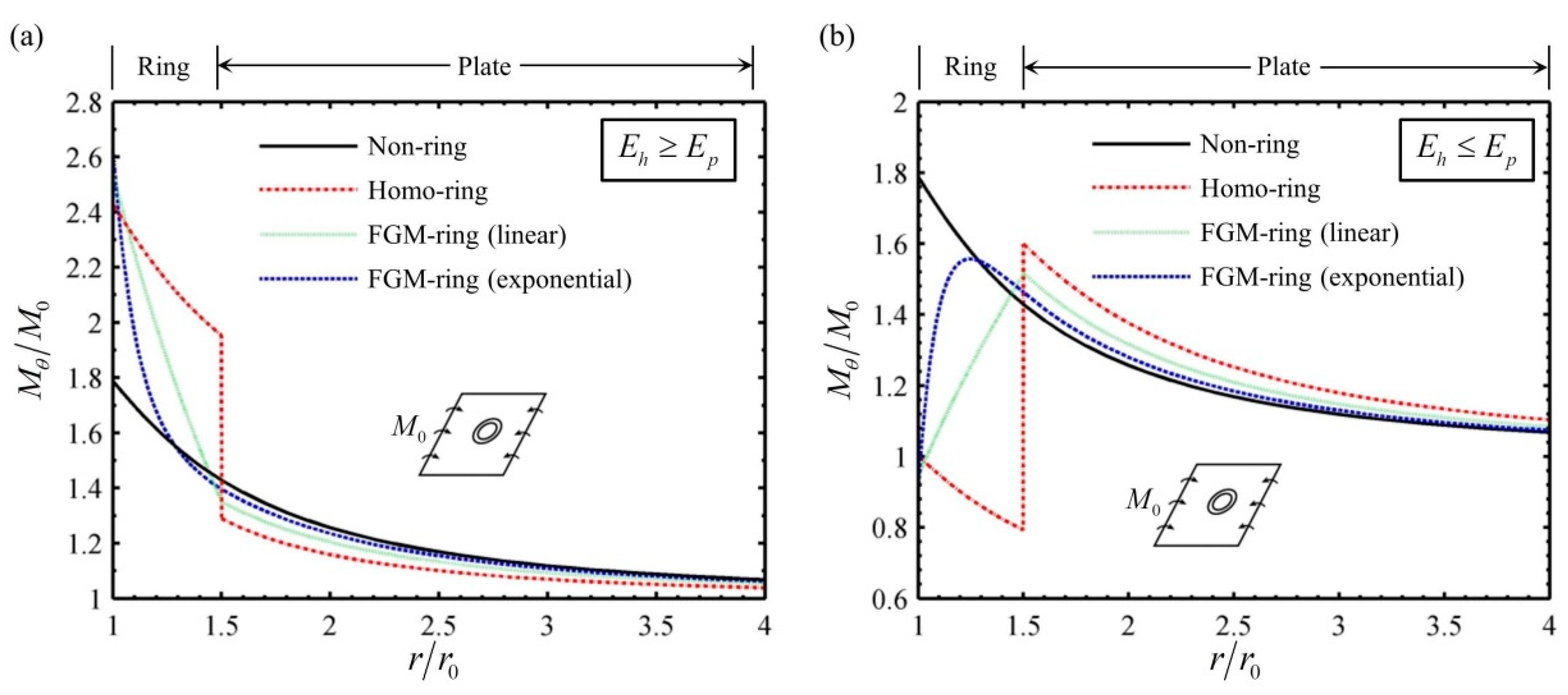
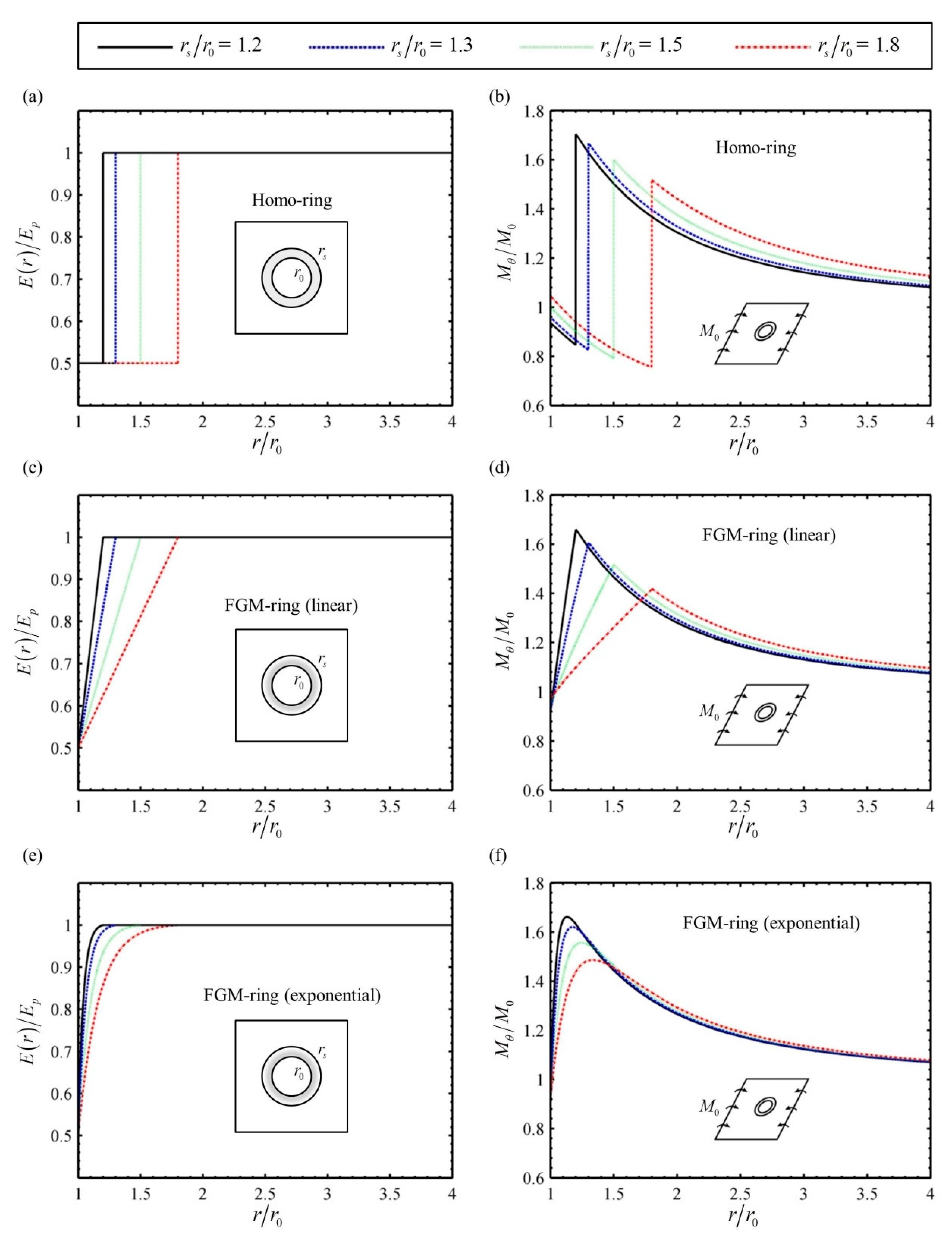
4.2. The Case for an FGM Ring Reinforced in a Homogeneous Plate

There is an important theoretical significance of the above conclusions on the bending stress concentration in a whole FGM plate. However, considering the feasibility of material preparation and engineering application, it would be better to reinforce a thin FGM ring around the hole to reduce the stress concentration, in comparison with manufacturing a whole FGM perforated plate [23]. Hence, the bending moments in a homogeneous plate with a circular hole reinforced with an FGM ring are further analyzed here. The schematic diagram of the structure is displayed in Figure 5a. The solution of the bending moments for this case can be easily derived by taking $r_s$ in Section 3 as the outer radius of the reinforcing ring.

Since the varying Poisson’s ratio has little effect on the bending moments, Poisson’s ratio is assumed as constant $\nu \left(r\right)={\nu }_0=0.3$ in the next discussions. Two Young’s moduli, $E_h$ at the edge of the hole and $E_p$ in the plate, are taken as the main parameters. Meanwhile, four types of the reinforcing ring listed in

Table 2. Four types of the reinforcing ring with different functions of Young’s modulus.

The Types of Ring	The Functions of Young’s Modulus
Non-ring	$E\left(r\right)=E_h=E_p$
Homo-ring	$E\left(r\right)=E_h\ne E_p$
FGM-ring (linear)	$E\left(r\right)=\left(E_p-E_h\right)\left(r-r_0\right)/\left(r_s-r_0\right)+E_h$
FGM-ring (exponential)	$E\left(r\right)=\left(E_p-E_h\right)/\left(1-e^5\right)\ast e^{5\left(1-\left(r-r_0\right)/\left(r_s-r_0\right)\right)}-\left(e^5{E}_p-E_h\right)/\left(1-e^5\right)$

are considered. The varying curves of Young’s modulus in four different reinforcing rings are presented in Figure 5b. The solid line in the figure represents a special case of a homogeneous plate with a circular hole with no ring. The dash-dotted line, dotted line, and dashed line mean the edge of the hole reinforced by, respectively, a homogeneous ring with unchanged Young’s modulus, FGM ring with linearly varying Young’s modulus, and FGM ring with exponentially varying Young’s modulus. It is obvious that Young’s modulus is always decreasing as $E_h>E_p$, but increasing as $E_h<E_p$ in Figure 5.

The distribution of bending moments $M_{\theta }/M_0$ for different types of the ring is presented in Figure 6 for the cases of $E_h\ge E_p$ and $E_h\le E_p$. The radius ratio of the ring is taken as $r_N/r_0=1.5$. It is observed from Figure 6a that the bending moments at the hole for three cases of “with-ring” are much higher than that of non-ring as Young’s modulus at the edge of the hole $E_h$ larger than that in the plate $E_p$. On the contrary, the moments near the hole for “with-ring” are less than that of non-ring as $E_h<E_p$ in Figure 6b. It is obvious that the moment concentration near the hole can be reduced in this case. However, it is also worth noting that the moments in the plate for “with-ring” are slightly higher than that of non-ring. For this reason, it is found that a sudden change of the moments occurs at the interface between the homogeneous ring and the plate. The sudden change of the moments will lead to a seriously interfacial stress concentration, which may promote the crack initiation and propagation along the interface and ultimately result in the failure of the whole structure. Therefore, the homogeneous ring can relieve the stress concentration near the hole, but the mismatch of material properties at the interface between the ring and the plate will cause a new interfacial stress concentration. The FGM ring can effectively avoid this problem due to continuous variations of elastic properties from the edge of the hole to the plate. It is clear evidence from the moment distribution in Figure 6b that the bending moment changes continuously in the ring and the plate with no jump for both linear FGM ring and exponential FGM ring. Meanwhile, both of them significantly reduce the moment concentrations near the hole. The only difference of the results between the linear and exponential FGM ring is the distribution shapes of the moment in the ring. The linear FGM ring causes the moment to vary along a linear way in the ring, while the exponential FGM ring causes a moment with a similarly exponential change.

Figure 7 shows the influence of the width of the reinforcing ring on the distribution of bending moment. It is supposed here the ratio of Young’s modulus $E_h/E_p=0.5$. Figure 7a,b show that the bending moments in the ring and the plate increase steadily as the width of the homogeneous ring increases. The difference of moments at the interface almost keeps constant. For the linear and exponential FGM rings in Figure 7c–f, the bending moments at the edge of the hole change very slightly as the width of the ring increases, but the maximum moment in the ring decreases gradually. Therefore, the increase of the widths of the ring is beneficial to reduce the overall moments in the structure. In particular, if the width of the ring is taken large enough in Figure 7f, the result will be reduced to the case of an infinite FGM plate with a circular hole as shown in Figure 3a.

Finally, the variations of SCF with the ratio of Young’s modulus $E_h/E_p$ and radius ratio $r_N/r_0$ are analyzed, and the results are shown in Figure 8 where the linear FGM ring is taken as an example. The SCF $K_{r_0}$ at the edge of the hole and $K_{r_N}$ in plate at the edge of the ring are defined as

$$K_{r_0}={(M_{r_0})}_{\max }/M_0,$$

(22)

$$K_{r_N}={(M_{r_s})}_{\max }/M_0,$$

(23)

where ${(M_{r_0})}_{\max }$ and ${(M_{r_s})}_{\max }$ are the maximum bending moments at the edge of the hole and in plate at the edge of the ring, respectively.

It is found from Figure 8a that the SCF $K_{r_0}$ grows quickly while $K_{r_N}$ decreases slowly as the abscissa $E_h/E_p$ increases. When $E_h/E_p>1$, that is the Young’s modulus at the edge of the hole is larger than that of the plate, the SCF $K_{r_0}$ is always higher than that of the homogeneous perforated plate. When $E_h/E_p<1$, the SCF in the structure attains the minimum value at the intersections of the curves of $K_{r_0}$ and $K_{r_0}$. The corresponding abscissas of the intersections are the optimal ratio of Young’s modulus to realize the minimum stress concentration.

It can be seen from Figure 8b that there is a special case as $E_h/E_p=$1.0, i.e., the Young’s modulus in the ring equal to that in the plate. The SCF $K_{r_0}$ remains constant and equal to 1.79, which is the result of a homogeneous plate with a circular hole. For other ratios of $E_h/E_p$, the SCF $K_{r_0}$ changes slowly with the abscissa $r_N/r_0$ increasing, while the SCF $K_{r_N}$ decreases rapidly in the approximate range $r_N/r_0=1\sim 2$ and then changes slightly as the abscissa $r_N/r_0$ increases. Hence, it can be concluded that the increase of the width of the ring is beneficial to relieve the bending stress concentration, but the effect will not be obvious after the width reaches a certain value.

5. Conclusions

Based on Muskhelishvili’s complex variable methods, the bending stress concentration at a circular hole in a functionally graded thin plate is analyzed. The method of piece-wise homogeneous layers is used to deal with the arbitrary variation of elastic properties along the radial direction in the plate. The effects of different variations of elastic parameters on the distribution of bending moments are discussed for two different cases: a whole FGM plate with a circular hole and an FGM ring reinforced in a homogeneous perforated plate. The following conclusions can be drawn.

(1)

For the case of a whole FGM plate, it is found that the bending stress concentration, caused by the geometric discontinuity of the hole in the traditional homogeneous plate, can be well relieved or even eliminated by choosing an appropriate radially increasing Young’s modulus in the plate. The radial change of Poisson’s ratio has little effect on reducing the bending stress concentration.

(2)

For the case of an FGM ring reinforced in a homogeneous plate, it is found the FGM reinforcing ring with radially increasing Young’s modulus can not only relieve the bending stress concentration around the hole, but also avoid the stress concentration at the interface between the ring and the plate compared with that of the homogeneous reinforcing ring.

(3)

The linear and exponential FGM rings can both reduce the stress concentration near the hole, and their effects are almost equally good. The only difference of their results are the distribution shapes of the bending moments. The linear FGM ring makes the moment vary along a linear way in the ring, while the exponential FGM ring brings the moment with a similarly exponential change.

(4)

The increase of the width of the reinforcing ring is beneficial to relieve the bending stress concentration, but the effect will not be obvious after the width reacheds a certain value.

References

1. Norton, R.L. Machine Design: An Integrated Approach; Prentice Hall: Boston, MA, USA, 2014. [Google Scholar]
2. Budynas, R.G.; Nisbett, J.K.; Shigley, J.E. Shigley’s Mechanical Engineering Design; McGraw-Hill: New York, NY, USA, 2020. [Google Scholar]
3. Young, W.C.; Budynas, R.G. Roark’s Formulas for Stress and Strain; McGraw-Hill: New York, NY, USA, 2002. [Google Scholar]
4. Pilkey, W.D.; Pilkey, D.F. Peterson’s Stress Concentration Factors; John Wiley & Sons, Inc.: Hoboken, NJ, USA, 2007. [Google Scholar]
5. Savin, G.N. Stress Concentration around Holes; Pergamon Press: New York, NY, USA, 1961. [Google Scholar]
6. Lekhnitskii, S.G. Anisotropic Plates; Gordon and Breach: New York, NY, USA, 1968. [Google Scholar]
7. Timoshenko, S.P.; Woinowsky-Krieger, S. Theory of Plates and Shells; McGraw-Hill: New York, NY, USA, 1959. [Google Scholar]
8. Yang, Q.; Gao, C.F. Reduction of the stress concentration around an elliptic hole by using a functionally graded layer. Acta Mech. 2016, 227, 2427–2437. [Google Scholar] [CrossRef]
9. Sburlati, R.; Atashipour, S.R.; Atashipour, S.A. Reduction of the stress concentration factor in a homogeneous panel with hole by using a functionally graded layer. Compos. Part B 2014, 61, 99–109. [Google Scholar] [CrossRef]
10. Goyat, V.; Verma, S.; Garg, R.K. Reduction in stress concentration around a pair of circular holes with functionally graded material layer. Acta Mech. 2018, 229, 1045–1060. [Google Scholar] [CrossRef]
11. Goyat, V.; Verma, S.; Garg, R.K. Reduction of stress concentration for a rounded rectangular hole by using a functionally graded material layer. Acta Mech. 2017, 228, 3695–3707. [Google Scholar] [CrossRef]
12. Udupa, G.; Rao, S.S.; Gangadharan, K.V. Functionally graded composite materials. An overview. Procedia Mater. Sci. 2014, 5, 1291–1299. [Google Scholar] [CrossRef]
13. Sburlati, R. Analytical elastic solutions for pressurized hollow cylinders with internal functionally graded coatings. Compos. Struct. 2012, 94, 3592–3600. [Google Scholar] [CrossRef]
14. Gupta, A.; Talha, M. Recent development in modeling and analysis of functionally graded materials and structures. Prog. Aerosp. Sci. 2015, 79, 1–14. [Google Scholar] [CrossRef]
15. Huang, J.; Venkataraman, S.; Rapoff, A.J.; Haftka, R.T. Optimization of axisymmetric elastic modulus distributions around a hole for increased strength. Struct. Multidiscip. Optim. 2003, 25, 225–236. [Google Scholar] [CrossRef]
16. Huang, J.; Rapoff, A.J. Optimization design of plates with holes by mimicking bones through nonaxisymmetric functionally graded material. P I Mech. Eng. L-J. Mater. 2003, 217, 23–27. [Google Scholar] [CrossRef]
17. Kubair, D.V.; Bhanu-Chandar, B. Stress concentration factor due to a circular hole in functionally graded panels under uniaxial tension. Int. J. Mech. Sci. 2008, 50, 732–742. [Google Scholar] [CrossRef]
18. Wang, W.; Yuan, H.; Li, X.; Shi, P. Stress concentration and damage factor due to central elliptical hole in functionally graded panels subjected to uniform tensile traction. Materials 2019, 12, 422. [Google Scholar] [CrossRef] [PubMed] [Green Version]
19. Yang, Q.; Gao, C.F.; Chen, W.T. Stress analysis of a functional graded material plate with a circular hole. Arch. Appl. Mech. 2010, 80, 895–907. [Google Scholar] [CrossRef]
20. Yang, Q.; Gao, C.F.; Chen, W.T. Stress concentration in a finite functionally graded material plate. Sci. China Phys. Mech. Astron. 2012, 55, 1263–1271. [Google Scholar] [CrossRef]
21. Mohammadi, M.; Dryden, J.R.; Jiang, L.Y. Stress concentration around a hole in a radially inhomogeneous plate. Int. J. Solids Struct. 2011, 48, 483–491. [Google Scholar] [CrossRef]
22. Goyat, V.; Verma, S.; Garg, R.K. On the reduction of stress concentration factor in an infinite panel using different radial functionally graded materials. Int. J. Mater. Prod. Technol. 2018, 57, 109–131. [Google Scholar] [CrossRef]
23. Sburlati, R. Stress concentration factor due to a functionally graded ring around a hole in an isotropic plate. Int. J. Solids Struct. 2013, 50, 3649–3658. [Google Scholar] [CrossRef] [Green Version]
24. Nie, G.J.; Zhong, Z.; Batra, R.C. Material tailoring for reducing stress concentration factor at a circular hole in a functionally graded material (FGM) panel. Compos. Struct. 2018, 205, 49–57. [Google Scholar] [CrossRef]
25. Kubair, D.V. Stress concentration factors and stress-gradients due to circular holes in radially functionally graded panels subjected to anti-plane shear loading. Acta Mech. 2013, 224, 2845–2862. [Google Scholar] [CrossRef]
26. Kubair, D.V. Stress concentration factor in functionally graded plates with circular holes subjected to anti-plane shear loading. J. Elast. 2014, 114, 179–196. [Google Scholar] [CrossRef]
27. Shi, P.P. Stress field of a radially functionally graded panel with a circular elastic inclusion under static anti-plane shear loading. J. Mech. Sci. Technol. 2015, 29, 1163–1173. [Google Scholar] [CrossRef]
28. Guan, Y.; Li, Y. Stress concentration and optimized analysis of an arbitrarily shaped hole with a graded layer under anti-plane shear. Appl. Sci. Basel 2018, 8, 2619. [Google Scholar] [CrossRef] [Green Version]
29. Yang, B.; Chen, W.Q.; Ding, H.J. 3D elasticity solutions for equilibrium problems of transversely isotropic FGM plates with holes. Acta Mech. 2015, 226, 1571–1590. [Google Scholar] [CrossRef]
30. Yang, B.; Chen, W.Q.; Ding, H.J. Equilibrium of transversely isotropic FGM plates with an elliptical hole: 3D elasticity solutions. Arch. Appl. Mech. 2016, 86, 1391–1414. [Google Scholar] [CrossRef]
31. Dave, J.M.; Sharma, D.S. Stresses and moments in through-thickness functionally graded plate weakened by circular/elliptical cut-out. Int. J. Mech. Sci. 2016, 105, 146–157. [Google Scholar] [CrossRef]
32. Muskhelishvili, N.I. Some Basic Problem of Mathematical Theory of Elasticity; Noordhoff: Groningen, The Netherlands, 1975. [Google Scholar]
Figure 1. A functionally graded thin plate with a circular hole subjected to remote bending moment.
Applsci 10 02231 g001
Figure 2. Variation of Young’s modulus and Poisson’s ratio along the radial direction.
Applsci 10 02231 g002
Figure 3. Distribution of moments M θ / M 0 for different varying Young’s modulus: (a) distribution along the radial direction under uniaxial bending ( θ = ± 90 0 ); (b) distribution around the hole under uniaxial bending; (c) distribution along the radial direction under balanced biaxial bending; (d) distribution around the hole under balanced biaxial bending.
Applsci 10 02231 g003
Figure 4. Distribution of moments M θ / M 0 around the hole for different varying Poisson’s ratio: (a) uniaxial bending; (b) balanced biaxial bending.
Applsci 10 02231 g004
Figure 5. (a) A homogeneous thin plate with a circular hole reinforced with a ring; (b) variation of Young’s modulus along the radial direction for four types of the ring.
Applsci 10 02231 g005
Figure 6. Distribution of moments M θ / M 0 along the radial direction ( θ = ± 90 0 ) for different types of ring: (a) E h = 1.5 E p ; (b) E h = 0.5 E p .
Applsci 10 02231 g006
Figure 7. Distribution of moments M θ / M 0 along the radial direction ( θ = ± 90 0 ) for different widths of ring: (a) variation of Young’s modulus for homogeneous ring; (b) distribution of moments for homogeneous ring; (c) variation of Young’s modulus for linear FGM ring; (d) distribution of moments for linear FGM ring; (e) variation of Young’s modulus for exponential FGM ring; (f) distribution of moments for exponential FGM ring
Applsci 10 02231 g007
Figure 8. Stress concentration factor (SCF) for a homogeneous plate with a circular hole reinforced with a linear FGM ring: (a) variation of SCF with E h / E p ; (b) variation of SCF with r s / r 0 .
Applsci 10 02231 g008