Shape Design Optimization of a Robot Arm Using a Surrogate-Based Evolutionary Approach

Abstract

In the design optimization of robot arms, the use of simulation technologies for modeling and optimizing the objective functions is still challenging. The difficulty is not only associated with the large computational cost of high-fidelity structural simulations but also linked to the reasonable compromise between the multiple conflicting objectives of robot arms. In this paper we propose a surrogate-based evolutionary optimization (SBEO) method via a global optimization approach, which incorporates the response surface method (RSM) and multi-objective evolutionary algorithm by decomposition (the differential evolution (DE ) variant) (MOEA/D-DE) to tackle the shape design optimization problem of robot arms for achieving high speed performance. The computer-aided engineering (CAE) tools such as CAE solvers, computer-aided design (CAD) Inventor, and finite element method (FEM) ANSYS are first used to produce the design and assess the performance of the robot arm. The surrogate model constructed on the basis of Box–Behnken design is then used in the MOEA/D-DE, which includes the process of selection, recombination, and mutation, to optimize the robot arm. The performance of the optimized robot arm is compared with the baseline one to validate the correctness and effectiveness of the proposed method. The results obtained for the adopted example show that the proposed method can not only significantly improve the robot arm performance and save computational cost but may also be deployed to solve other complex design optimization problems.

1. Introduction

Nowadays, facing the megatrend for smart factories of the future, industrial robots play a greatly important role not only in traditional pick-and-place tasks but also in many of the precision applications such as assembly, welding, and machining. These robots, in order to satisfy the requirements of new applications, must be designed to meet high end/performance requirements, i.e., high accuracy and high efficiency. The design process of an industrial robot arm with high speed performance is still challenging due to the interconnecting roles of adjacent joints, which may significantly impact the efficiency and stability of the robot arm. For example, the deformation and residual vibration of the robot arm will cause its positioning accuracy to decrease, and the robot arm mass and moment of inertia will affect its dynamic behavior, such as controllability and efficiency; moreover, these factors generally are in conflict with each other. Therefore, design optimization of robot arms is becoming increasingly important.

With the advance of digital twins in smart factories, the use of simulation technologies to address computation-expensive and multi-objective optimization issues has become an important research topic. Design optimization is the process of establishing the right combination of product parameters that satisfy project requirements [1]. Structural optimization can be separated into three main categories: size, shape, and topology optimization [2]. In a structural design process, a topology optimization is first performed to obtain an initial sketch of the optimal configuration of the structure; the suggested configuration is interpreted to draw an engineering design, and this design is then optimized using detailed sizing and shape optimization methods together with realistic design constraints. These methods are not only able to optimize the robot arm but can also be extended to the design of the whole robot system. For the purpose of improving the performance of industrial robots, a number of research works have been carried out with respect to the related topics in recent years. Some works focused on the selection criteria of the servo motor and gearbox for optimizing the servo drive system [3,4]. A few reports studied new control algorithms to obtain high speed performance, such as residual vibration suppression [5]. Certain researchers used the finite element method (FEM) to optimize robot structure. Roy et al. used the finite element method to design a high-performance robot arm and reported experimental structural data to support the design of the robot arm [6]. Park and Asada studied the design optimization of the mechanical structure and control of a two-link robot for which the weight and inertia of the robot arm were minimized to attain high-speed positioning [7]. Sahu and Choudhury used the FEM of the ANSYS workbench to optimize the performance of a six-axis industrial robot via stress, modal, and dynamic behavior analyses [8,9,10]. Pupăză et al. also used an FEM-based optimization technique to study the influence of the static and dynamic behaviors on the positioning accuracy of robots [11]. Chen et al. analyzed the static strength and stiffness of a two-link robot and then used a topology optimization method to design the structure for quality improvement [12]. In the above studies, it was revealed that CAE together with FEM-based design optimization can be an important tool for attaining structural performance improvement in real-world engineering applications. However, for cases with large design space or the requirement of attaining numerous design samples, the high computational effort of analysis may hinder the implementation of the conventional FEM-based design optimization methods in the design optimization process. On the other hand, only a few researchers have studied the multi-objective and computational inefficiency problems related to the design optimization of industrial robots.

The response surface method (RSM), also known as the surrogate model or approximation model, can be used to improve the design efficiency. In RSM, a set of sample data (obtained by running the computer code/simulation) are used to build the surrogate model, which are sufficient to predict the output at untried points within the design space. Because the predictions obtained from a surrogate model are generally much more efficient than those from numerical analysis code, the computational cost associated with each search in RSM is therefore negligible. Surrogate-model-based optimizations are of particular interest for engineering design when coupled with high-fidelity and expensive analysis codes, such as computation fluid dynamics (CFD) and computational structural dynamics (CSD) [13]. In many studies, RSM together with design of experiment (DOE) was used to construct the surrogate models and find the best-fitting solutions [14,15,16,17]. Some researchers applied the adaptive RSM to search for the global optima of complex mechanical systems [18,19,20]. However, in these cases, they did not consider the situation of multi-objective functions with conflicting properties [21] which may lead to being trapped into a local optimum solution during the design optimization process.

In this paper, the shape design optimization of robot arms for high speed performance via the surrogate-based evolutionary approach is investigated. First, based on the CAD model of a robot arm, the design variables, constraints, and objective functions of the optimization problem are defined. Next, a quadratic RSM together with Box–Behnken design (BBD) and FEM is used to construct the surrogate model. In solving the optimization problem, the multi-objective evolutionary algorithm by decomposition (DE variant) (MOEA/D-DE) technique which includes evolutionary operators of selection, recombination, and mutation is employed to address the multiple objective functions with conflicting features and search for the Pareto-optimal sets of global optimization. The weighted sum method is finally used to determine the best candidate among the generated population samples through fitness checking. The proposed paper is able to make two significant contributions: one is to provide a surrogate-based evolutionary optimization approach to deploy in the robot arm design optimization process to obtain higher performance and efficiency, as well as to reduce computational cost; the other one is to solve the shape design optimization problem of robot arms considering multiple, conflicting objectives for higher accuracy and controllability simultaneously.

The rest of the paper is organized as follows. The techniques for robot arm analysis and design, which involve the target performance to be achieved and the framework of the proposed surrogate-based evolutionary optimization (SBEO) method, are described in Section 2. The procedure for the optimal shape design of a specific robot arm is given in Section 3. Some optimal-design-related simulation results, such as Pareto front history, improvement of performance, computational efficiency, and sensitivity analysis, are given in Section 4. Section 5 presents a discussion on the advantages, limitations, and future works of the proposed method.

2. Techniques for Robot Arm Analysis and Design

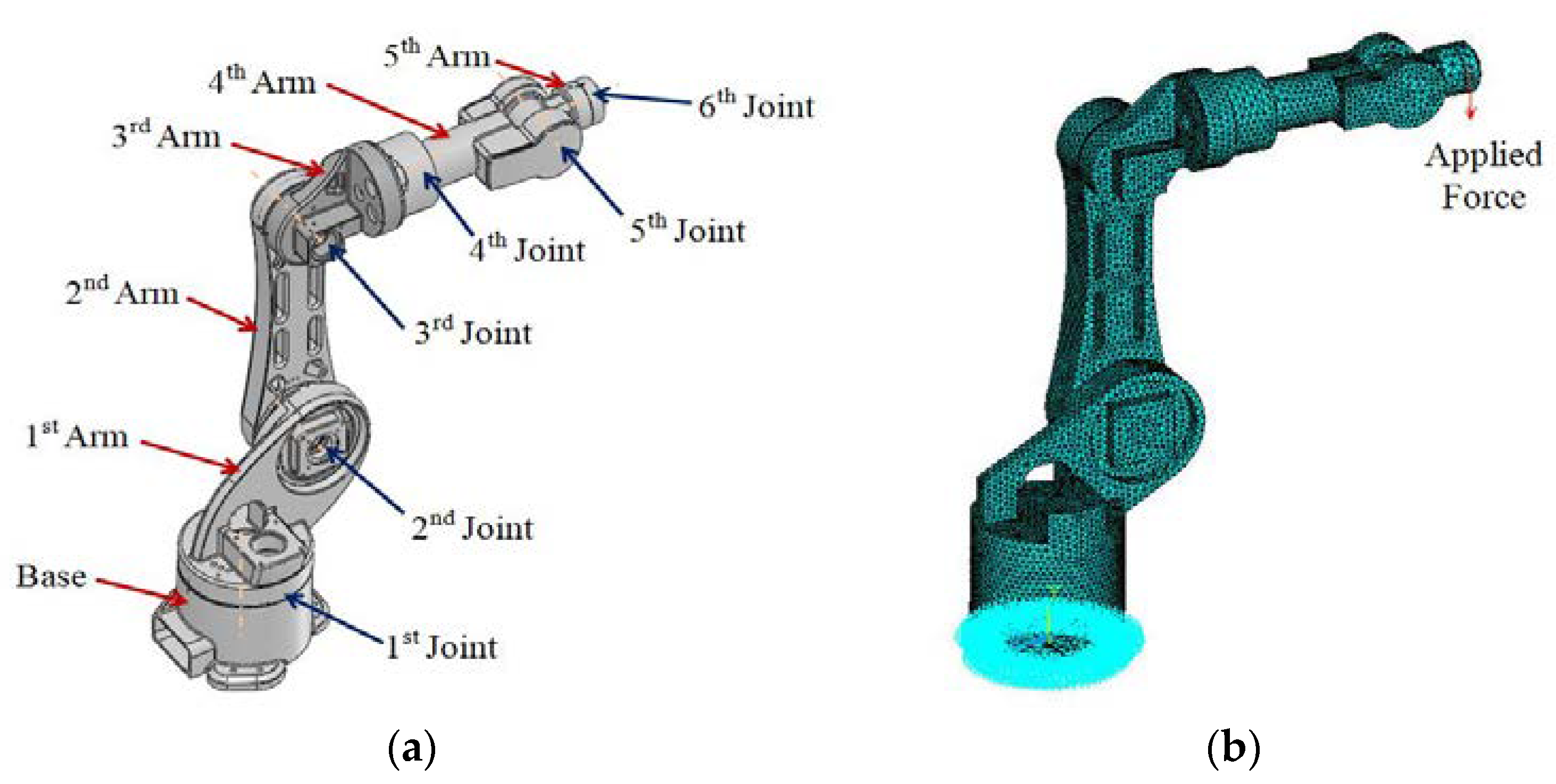
2.1. Architecture of the Industrial Robot

The PMC6VA030 robot, the six-axis vertical articulated industrial manipulator shown in Figure 1, is fabricated by PMC, Taiwan. The maximum payload and reach of the robot are 30 kg and 1800 mm, respectively. The architecture of the robot is composed of six revolute joints and six robot arms. Each robot arm is driven by a joint module which consists of a servo motor, reduction gear, and encoder.

2.2. Problem Description of the Robot Arm

The accuracy, controllability, and efficiency are important performance aspects of a high-speed industrial robot. Due to the robot arms playing roles of interconnection between the adjacent joints, their characteristics are able to influence the system performance very well. When the power capacities of the joint modules are fixed, the shape dimensions of the robot arms are able to significantly affect the robot performance. Therefore, shape design optimization of the robot arms to obtain the minimum weight, maximum stiffness, and minimum deformation must be accomplished [22]. Figure 2a is a detailed engineering drawing of the baseline 2nd robot arm which includes all of the shape dimensions in it. A schematic view of the proposed 2nd robot arm with the chosen design variables is shown in Figure 2b. The unspecified dimensions on this sketch are all the same as those in Figure 2a and will not be optimized in this article under real engineering consideration.

2.2.1. Objective Functions

In this paper, the weight (W), moment of inertia (J), and deformation (D) of the 2nd robot arm were chosen as tri-objective functions. The mathematical model of the multi-objective optimization problem is as follows [23]:

$$\mathrm{minimize} \mathrm{F}\left(\mathrm{X}\right)={\left(\mathrm{W}\left(\mathrm{X}\right), \mathrm{J}\left(\mathrm{X}\right),\mathrm{D}\left(\mathrm{X}\right)\right)}^{\mathrm{T}}$$

(1)

$${\mathrm{subject} \mathrm{to} \mathrm{h}}_{\mathrm{i}}\left(\mathrm{X}\right)=0 \mathrm{i}=1,2,\dots ,\mathrm{p}$$

(2)

$${ \mathrm{g}}_{\mathrm{j}}\left(\mathrm{X}\right)\le 0 \mathrm{j}=1,2,\dots ,\mathrm{q}$$

(3)

$${\mathrm{x}}_{\mathrm{L}}\le \mathrm{X}\le {\mathrm{x}}_{\mathrm{U}} \mathrm{X}={\left({\mathrm{x}}_1,{\mathrm{x}}_2,\dots ,{\mathrm{x}}_{\mathrm{n}}\right)}^{\mathrm{T}}$$

(4)

where F(X), h(X), and g(X) are, respectively, the objective functions and the equality and inequality constraint functions; X ∈ Rⁿ is a vector of n design variables; p and q are the numbers of constraint functions.

The multi-objective optimization problem can be expressed as a single equation via weighted sum and normalization:

$${\mathrm{minimize} \mathrm{F}}_{\mathrm{j}}\left(\mathrm{X}\right)=w_1\times \frac{\mathrm{Min} \mathrm{W}}{{\mathrm{W}}_{\mathrm{j}}}+w_2\times \frac{\mathrm{Min} \mathrm{J}}{{\mathrm{J}}_{\mathrm{j}}}+w_3\times \frac{\mathrm{Min} \mathrm{D}}{{\mathrm{D}}_{\mathrm{j}}}$$

(5)

where j = 1, 2, 3, …., ps, and ps is the population size. w₁, w₂, and w₃ are weighted factors for preference criteria.

2.2.2. Design Variables

Several independent geometric parameters of the 2nd robot arm, including shape dimension initial point H_i, position of inflection point H_m and V_m, radius of opening R_h, and arm thickness T_a, were chosen as the design variables. The ranges of the design variables in the evolutionary models are shown in

Table 1. Ranges of design variables in the evolutionary model.

Design Variable		Model-1		Model-2		Model-3
		xiL	xiU	xiL	xiU	xiL	xiU
Shape Dimension (point A)	Hi	100	250	150	200	150	200
Shape Dimension (point C)	Hm	400	560	450	550	450	550
Shape Dimension (point C)	Vm	100	120	100	120	100	120
Radius of Reduced Hole	Rh	40	60	50	60	50	60
Thickness of Robot Arm	Ta	100	120	90	110	90	100

.

For statistical calculations, X_i is related to x_i via the following equation:

$$X_{\mathrm{i}}=\frac{{\mathrm{x}}_{\mathrm{i}}-{\mathrm{x}}_0}{\left({\mathrm{x}}_{\mathrm{iU}}-{\mathrm{x}}_{\mathrm{iL}}\right)/2} \mathrm{i}=1,2,3$$

(6)

where X_i is the coded value of a dimensionless design variable which can be easily calculated; x_i is the actual value of a design variable; x₀ is the actual value of a design variable at the center point; and x_iU and x_iL are the upper and lower bounds of a design variable.

2.2.3. Design Constraints

The above objective functions are subject to design constraints which are related to the geometry and mechanical behavior of the robot arm.

• The first set of constraints is the limitation of the feasible design region for design variables based on Table 1.

  $${\mathrm{x}}_{\mathrm{iL}}<x_{\mathrm{i}}<{\mathrm{x}}_{\mathrm{iU}}$$

  (7)
• The second set of constraints considers the relationship between the radius R_c of the circumcircle and design variables H_i, H_m, and V_m. According to the formulation of the circumcircle, the coordinates (x, y) of the circumcenter of a triangle and its radius R_c can be obtained as follows.

  $$\mathrm{x}=\frac{\left|\begin{array}{ccc}{H}_i^2+{155}^2& 155& 1\\ H_m^2+V_m^2& V_m& 1\\ {770}^2+{125}^2& 125& 1\end{array}\right|}{2\times \left|\begin{array}{ccc}{H}_i& 155& 1\\ H_m& V_m& 1\\ 770& 125& 1\end{array}\right|} \mathrm{mm} , \mathrm{y}=\frac{\left|\begin{array}{ccc}{H}_i& H_i^2+{155}^2& 1\\ H_m& {\mathrm{H}}_{\mathrm{m}}^2+{\mathrm{V}}_{\mathrm{m}}^2& 1\\ 770& {770}^2+{125}^2& 1\end{array}\right|}{2\times \left|\begin{array}{ccc}{H}_i& 155& 1\\ H_m& V_m& 1\\ 770& 125& 1\end{array}\right|} \mathrm{mm}$$

  (8)

  $${\mathrm{R}}_{\mathrm{c}}=\sqrt{{\left(\mathrm{x}-H_i\right)}^2+{\left(\mathrm{y}-155\right)}^2 } \mathrm{mm}$$

  (9)

  Hence, the constraint involving y should be

  $${\mathrm{g}}_1\left(x\right)={\mathrm{R}}_{\mathrm{c}}-\mathrm{y}+80<0 \mathrm{mm}.$$

  (10)
• One constraint is related to the weight-to-stiffness ratio (W2SR), which is a measure of material mass efficiency used to provide unit resistance to elastic deformation. An improved W2SR enables the realization of longer spans without incurring a significant cost penalty, which is expressed in terms of material usage and deflections due to weight [24]. The W2SR computed from the weight and stiffness of a robot arm can be expressed as

  $$\mathrm{W}2\mathrm{SR}=\mathrm{f}\left(\mathrm{W},\mathrm{D},{\mathrm{F}}_{\mathrm{y}}\right)=\frac{\left(\mathrm{W}\times \mathrm{D}\right)}{{\mathrm{F}}_{\mathrm{y}}} \left(u\mathrm{m}\right)$$

  (11)

  where F_y is the applied force at the distal-end joint.
• Another constraint is related to the weight-to-moment-of-inertia ratio (W2JR), a measure of a structural property. A higher W2JR will push resonance and anti-resonance peaks to lower frequencies, shrinking the operating bandwidth of the machine. The measure of W2JR in this paper is obtained as

  $$\mathrm{W}2\mathrm{JR}=\mathrm{f}\left(\mathrm{W},\mathrm{J}\right)=\frac{\mathrm{W}}{\mathrm{J}}({\mathrm{m}}^2).$$

  (12)

The above two measures of W2SR and W2JR are both “the smaller the better” when the design optimization of robot arms is targeting higher accuracy and controllability. Two additional constraints imposed on the objective functions are as follows:

$${\mathrm{g}}_2\left(\mathrm{x}\right)=\mathrm{W}2\mathrm{SR}-12<0,$$

(13)

$${\mathrm{g}}_3\left(\mathrm{x}\right)=\mathrm{W}2\mathrm{JR}-8<0.$$

(14)

2.3. Performance Analysis Using a CAE Solver

The performance of the robot arm was analyzed using a CAE solver in this paper. The model of an industrial robot built using Autodesk Inventor 3D CAD software was imported into the ANSYS MechanicalANSYS Parametric Design Language (APDL )FEM solver in the “*.STP” format. The material of the robot arm is aluminum 6061 with modulus of elasticity E = 69 GPa, density ρ = 2700 kg/m³, and Poisson’s ratio ν = 0.3, applied force at the distal-end joint F_Y = 1300 N, moment M_X = 277 Nm, and M_Z = 512 Nm.

The 2nd robot arm, together with the subsequent arms and distal-end joint, is shown in Figure 3a. All the subsequent arms are treated as point masses (also known as remote forces) which are used to transfer the force at the distal-end joint (right side) to the 2nd robot arm. Consequently, a resultant force F_Y and two resultant moments M_X and M_Z are applied to the 2nd robot arm as shown in Figure 3b.

The FEM mesh of the 2nd robot arm is shown in Figure 4a, and the supporting boundary is placed at the proximal end (left side) of the robot arm with the harmonic reducer treated as a fixed connection as shown in Figure 4b. The FEA results are shown in Figure 5.

2.4. The Proposed SBEO Approach

2.4.1. The Framework and Procedure

In this paper we propose a surrogate-based evolutionary optimization (SBEO) method which integrates surrogate models with the multi-objective evolutionary algorithm based on decomposition (MOEA/D-DE). A conceptual sketch is shown in Figure 6. The evolutionary optimization is carried out in the Python programming language using the “PyGMO” open-source optimization library. Herein, we will only give a brief introduction, and the reader can refer to [25,26] for more details.

The procedure of the proposed SBEO method is outlined in the following steps:

(1)

First, a DOE plan is built based on the Box–Behnken design, and initial sample points are chosen according to the plan matrix. The objective (performance) functions are then analyzed and evaluated using the ANSYS solver following the baseline design CAD model of the robot arm.

(2)

A quadratic polynomial regression model is defined as the surrogate model for the objective functions based on the sampled dataset. The model parameters are then solved by inverse matrix transformation using Python’s numpy library’s “Polynomial.fit” function.

(3)

The surrogate model is used to search for the optimal solution of the objective subjected to the constraint functions in the design space using the MOEA/D-DE algorithm.

(4)

The weighted sum method, in which each weighting factor is chosen according to the importance or preference of each objective, is then used to determine the best candidate among the generated population samples. These candidates are used to evaluate the fitness with the termination conditions given in Equations (15)–(17). The reduced design space is thereby found to update the surrogate model.

(5)

Steps 3 and 4 are repeated until one of the termination conditions is satisfied.

2.4.2. Criteria of Model Renewal and Termination

The first termination condition is about the distance between samples and difference of their objective responses:

$$\Vert x_{\mathrm{new}}-x_{\mathrm{best}}\Vert /\Vert x_{\mathrm{best}}\Vert \le {\mathsf{\epsilon }}_1,$$

(15)

$$\Vert y_{\mathrm{new}}-y_{\mathrm{best}}\Vert /\Vert y_{\mathrm{best}}\Vert \le {\mathsf{\epsilon }}_2.$$

(16)

The second one is about the maximum number of affordable expensive function evaluations:

$$\mathrm{N}\le {\mathrm{N}}_{\max }.$$

(17)

In general, if one of the preceding conditions is reached, the optimization is terminated [27].

According to the main effect analysis of DOE in obtaining the sensitivity of design variables, a selected reduced design space is used to renew the RS models. When one of the termination criteria given in Equations (15)–(17) is satisfied, the iterations for model renewing will stop.

3. Shape Design Optimization of the 2nd Robot Arm

3.1. Design Procedure of RSM with BBD

The design procedure of the response surface method in association with Box–Behnken design is as follows:

(1)

Identify the definition and the value of each variable;

(2)

Create a Box–Behnken design matrix;

(3)

Define a polynomial regression model;

(4)

Set up the X-Table in design of experiment (DOE);

(5)

Convert X to physical values x = mean of x + X × standard deviation of x (σ_x);

(6)

Assess y using FEA and the CAD model;

(7)

Compute the approximations of mean of y and range of y for scaling Y;

(8)

Convert y to scaled Y: Y = (y−mean of y)/(range of y/2);

(9)

Solve beta coefficients;

(10)

Compare model y = [x] × {beta Coefficient} with analytical (“exact”) y for validation.

3.2. Construction of the BBD Matrix

Box–Behnken design is a rotatable second-order design based on three-level incomplete factorial designs, which can decrease the number of experiments to reduce laboratory work. A detailed description of the method can be found in [28]. Herein, a three-factor and three-level Box–Behnken design matrix with 46 runs was chosen as the basic form of the RSM. The Model-3 case is shown in

Table 2. Box–Behnken design matrix with data for Model-3.

Run	Coded Variables					Uncoded (Real) Variables					Response (FEM)
	X1	X2	X3	X4	X5	Hi(x1)	Hm(x2)	HV(x3)	Rh(x4)	Ta(x5)	W(y1)	J(y2)	D(y3)
1	−1	−1	0	0	0	150	450	110	55	95	37.8640	7.4954	0.03921
2	−1	1	0	0	0	150	550	110	55	95	38.3861	7.6226	0.03809
3	1	−1	0	0	0	200	450	110	55	95	38.4216	7.4789	0.03700
4	1	1	0	0	0	200	550	110	55	95	39.2435	7.6958	0.03555
5	0	0	−1	−1	0	175	500	100	50	95	37.0219	7.1141	0.04079
6	0	0	−1	1	0	175	500	100	60	95	36.0889	7.0655	0.04287
7	0	0	1	−1	0	175	500	120	50	95	41.1573	8.1635	0.03313
8	0	0	1	1	0	175	500	120	60	95	40.2243	8.1149	0.03449
9	0	−1	0	0	−1	175	450	110	55	90	35.3401	6.8625	0.04671
10	0	−1	0	0	1	175	450	110	55	100	41.6777	8.2743	0.03387
11	0	1	0	0	−1	175	550	110	55	90	35.9760	7.0237	0.04520
12	0	1	0	0	1	175	550	110	55	100	42.3765	8.4515	0.03272
13	−1	0	−1	0	0	150	500	100	55	95	36.1010	7.0679	0.04390
14	−1	0	1	0	0	150	500	120	55	95	40.4444	8.1267	0.03446
15	1	0	−1	0	0	200	500	100	55	95	37.0302	7.1134	0.04001
16	1	0	1	0	0	200	500	120	55	95	40.9697	8.1538	0.03308
17	0	0	0	−1	−1	175	500	110	50	90	36.2567	7.0050	0.04481
18	0	0	0	−1	1	175	500	110	50	100	42.6410	8.4286	0.03238
19	0	0	0	1	−1	175	500	110	60	90	35.3237	6.9565	0.04663
20	0	0	0	1	1	175	500	110	60	100	41.7079	8.3801	0.03383
21	0	−1	−1	0	0	175	450	100	55	95	36.0959	6.9702	0.04304
22	0	−1	1	0	0	175	450	120	55	95	40.2101	8.0121	0.03441
23	0	1	−1	0	0	175	550	100	55	95	36.6138	7.1004	0.04158
24	0	1	1	0	0	175	550	120	55	95	41.0175	8.2187	0.03330
25	−1	0	0	−1	0	150	500	110	50	95	38.7225	7.6191	0.03744
26	−1	0	0	1	0	150	500	110	60	95	37.7895	7.5705	0.03960
27	1	0	0	−1	0	200	500	110	50	95	39.4499	7.6557	0.03535
28	1	0	0	1	0	200	500	110	60	95	38.5168	7.6072	0.03673
29	0	0	−1	0	−1	175	500	100	55	90	33.8264	6.4804	0.05110
30	0	0	−1	0	1	175	500	100	55	100	40.0143	7.8544	0.03724
31	0	0	1	0	−1	175	500	120	55	90	37.7877	7.4856	0.04164
32	0	0	1	0	1	175	500	120	55	100	44.3674	8.9590	0.03004
33	−1	0	0	0	−1	150	500	110	55	90	35.4554	6.9641	0.04696
34	−1	0	0	0	1	150	500	110	55	100	41.8044	8.3859	0.03422
35	1	0	0	0	−1	200	500	110	55	90	36.1521	6.9992	0.04450
36	1	0	0	0	1	200	500	110	55	100	42.5701	8.4245	0.03202
37	0	−1	0	−1	0	175	450	110	50	95	38.6021	7.5130	0.03721
38	0	−1	0	1	0	175	450	110	60	95	37.6691	7.4644	0.03895
39	0	1	0	−1	0	175	550	110	50	95	39.2660	7.6813	0.03599
40	0	1	0	1	0	175	550	110	60	95	38.3329	7.6328	0.03761
41	0	0	0	0	0	175	500	110	55	95	38.6488	7.6147	0.03700
42	0	0	0	0	0	175	500	110	55	95	38.6488	7.6147	0.03700
43	0	0	0	0	0	175	500	110	55	95	38.6488	7.6147	0.03700
44	0	0	0	0	0	175	500	110	55	95	38.6488	7.6147	0.03700
45	0	0	0	0	0	175	500	110	55	95	38.6488	7.6147	0.03700
46	0	0	0	0	0	175	500	110	55	95	38.6488	7.6147	0.03700

.

3.3. Formulation of the RS Regression Model

The response surface method is used to construct a suitable approximation of the true functional relationship between a dependent variable (the response) and a vector of independent variables. The response is generally evaluated experimentally or analyzed using numerical simulation [29].

A quadratic regressive equation was chosen to be the model of the robot arm, as shown below:

$$Y={\beta }_0+{\displaystyle \sum }_{i=1}^n{\beta }_i{x}_i+{\displaystyle \sum }_{i=1}^{n-1}{\displaystyle \sum }_{j=i+1}^n{\beta }_{ij}{x}_i{x}_j+{\displaystyle \sum }_{i=1}^n{\beta }_{ii}{x}_i^2+\epsilon$$

(18)

where Y is the response or performance function, x_i, x_j are the decision variables, β_o is the offset term, β_i represents the linear term, β_ii denotes the quadratic term, β_ij denotes the interactive term, and ε is the statistical error. The relationship between the coded and real variables is described in Equation (8). The values of β are obtained from Equation (19) using inverse matrix transformation by Python’s numpy library’s “Polynomial.fit” function as below:

$$\beta ={\left(X^T\ast X\right)}^{-1}\ast X^T\ast Y.$$

(19)

3.4. Calculation of the Coefficients of the RS Model

The coefficients of different surrogate models obtained via Equation (18) and the real variables obtained by the transformation of the coded variables are shown in

Table 3. The coefficients of RS models and real variables.

Coded Variables		Model-1			Model-2			Model-3
Model Coefficients		YW	YJ	YD	YW	YJ	YD	YW	YJ	YD
Beta 0	Const.	0.02734	0.02496	−0.15331	−0.00590	−0.00610	−0.15458	−0.01057	−0.01064	−0.01826
Beta 1	x1	0.11596	0.00428	−0.37509	0.04264	0.00331	−0.10549	0.06862	0.01394	−0.11655
Beta 2	x2	0.09879	0.11059	−0.18021	0.03929	0.03783	−0.05495	0.06323	0.06838	−0.06151
Beta 3	x3	0.25687	0.28164	−0.46145	0.24607	0.27069	−0.32638	0.39591	0.42706	−0.39148
Beta 4	x4	−0.08976	−0.02008	0.14201	−0.05228	−0.01179	0.06951	−0.08852	−0.01959	0.08057
Beta 5	x5	0.74737	0.72229	−0.56288	0.75449	0.72972	−0.79298	0.60527	0.57397	−0.60071
Beta 6	x12	−0.01362	−0.00941	0.10906	−0.00099	0.00532	0.01938	−0.00159	−0.00037	0.01376
Beta 7	x22	0.06079	0.08144	−0.07636	0.00885	0.03363	−0.00680	0.01422	0.01810	−0.00774
Beta 8	x32	−0.03279	−0.00272	0.17937	−0.01193	−0.00233	0.05312	−0.01916	−0.00370	0.05953
Beta 9	x42	0.00000	0.00000	−0.08645	0.00000	0.00000	−0.01540	0.00000	0.00000	−0.01861
Beta 10	x52	0.01099	0.00108	0.04749	0.00410	0.00088	0.01302	0.00327	0.00070	0.00623
Beta 11	x1x2	−0.05798	−0.06420	0.11599	−0.01896	−0.01527	0.03603	−0.03051	−0.03286	0.03191
Beta 12	x1x3	0.00505	0.00647	0.05851	0.00853	0.00978	0.00752	0.01373	0.01541	0.00848
Beta 13	x1x4	0.00000	0.00000	−0.00978	0.00000	−0.00003	−0.00237	0.00000	0.00000	−0.00287
Beta 14	x1x5	0.00865	0.00949	0.02232	0.00373	0.00408	0.01182	0.00298	0.00322	0.00833
Beta 15	x2x3	0.00033	0.00181	0.07972	−0.00051	−0.00123	0.03799	−0.00081	0.00096	0.06871
Beta 16	x2x4	0.00000	0.00000	−0.02389	0.00000	0.00000	−0.01404	0.00000	0.00000	−0.01702
Beta 17	x2x5	0.02283	0.02510	0.05574	0.02318	0.02548	−0.01720	0.01858	0.02005	0.05375
Beta 18	x3x4	−0.00816	−0.00108	0.03197	−0.00234	−0.00238	0.01659	−0.00398	−0.00095	0.01111
Beta 19	x3x5	0.00000	0.00000	−0.02829	0.00003	0.00000	−0.01601	0.00000	0.00000	−0.00895
Beta 20	x4x5	0.00082	0.00112	0.10402	0.03974	0.03661	0.33444	0.06728	0.06380	0.21738
Real Variable yi = Yi× y_Range/2 + y_Mean i = W, J, D
y_Mean		49.29504	9.91004	0.02896	42.24819	8.41802	0.03467	38.70456	7.62786	0.04325
y_Range/2		9.45013	2.17960	0.00726	8.92588	2.05787	0.01077	5.27049	1.23931	0.01053

.

3.5. Validation of the RS Model

In statistical analysis, the coefficient determination of R² [30] is a measure used to assess how well a model can explain and predict outcomes. It is also commonly known as “R-squared”, to be used as a guideline for measuring the accuracy of the model. It ranges from 0 to 1 and will be closer to 1 when the model is more precise. Joglekar and May [31] suggested that the value of R² for the best-fitting model should be at least 0.8. According to each DOE matrix, the obtained model is able to produce a predicted response (called Y_Model). The analyzed response produced by the CAE solver is called Y Exact. If these two values are equal, the red points in Figure 7 will lie on the diagonal line. The R² values of W, J, and D models being, respectively, 0.9875, 0.9865, and 0.9229 mean that the surrogate models evaluated in this study can be used to explain the W, J, and D very well.

3.6. Multi-objective Evolutionary Optimization

The use of MOEA/D-DE algorithm for solving multi-objective optimization in robot arm design allows us to find the Pareto front and the corresponding optimal parameter sets. The surrogate models in Table 2 were substituted into the MOEA, MOEA/D-DE operators with the adoption of the following parameters:

(1)

Generations = 300;

(2)

Weight generation = grid → method to generate the weights;

(3)

Decomposition method = Tchebycheff → method used to decompose the objectives;

(4)

Neighbor = 20 → size of weights neighborhood;

(5)

Crossover parameter = 0.9;

(6)

Differential evolution parameter = 0.5;

(7)

Distribution index = 20 → used for polynomial mutation;

(8)

Real b = 0.9 → chance that the neighborhood is considered at each generation, rather than the whole population (part of the diversity preservation mechanism);

(9)

Limit = 2 → number of copies reinserted in the population (part of the diversity preservation mechanism);

(10)

Preserve diversity = True → diversity preservation mechanisms.

We also set the preference criteria shown in Equation (5) as w₁ = 0.4, w₂ = 0.35, w₃ = 0.25 and in Equations (15) and (16) as ε₁ = ε₂ = 5%. A flowchart of the MOEA/D-DE algorithm for multi-objective optimization is shown in Figure 8.

4. Simulation Results

The optimization problem stated in Equations (1)–(4) for the optimal shape design of the 2nd robot arm was solved using the proposed method. The results related to the optimal design are given in the following to illustrate the effectiveness and feasibility of the proposed method.

4.1. Pareto Front History

In solving a multi-objective optimization problem, a solution that has one or several objective functions that are impossible to further optimize while other objective functions are not deteriorating is called “Pareto optimal” [32]. In this case, the Pareto front history of MOEA is plotted in Figure 9, and it is obvious that the solution started to converge at the 10th generation of MOEA.

4.2. Weighted Sum History

The multi-objective optimization problem of Equation (5) was evaluated to obtain the weighted sum result. The objectives and design variables in different models and generations according to the preference criteria on the optimal candidate in each generation of MOEA are shown in Figure 10a and Figure 10b. Optimal values for W of 33.02 kg, J of 6.3328 kg.m², and D of 0.0491 mm were obtained for H_i = 198.81 mm, H_m = 549.99 mm, V_m = 100.07 mm, R_h = 60.00 mm, and T_a = 90.13 mm.

4.3. The Improvement of Performance

The predicted optimal parameter sets for the models of the 2nd robot arm obtained in the SBEO process were analyzed using ANSYS to obtain the responses of the selected objectives, which were then compared with those of the baseline design. The results of different models are shown in

Table 4. Comparison of objectives with the baseline design.

2nd Robot Arm	Objectives (Predicted by Model/ANSYS)
	Weight W (kg)	Moment of Inertia J (kg. m2)	Deformation D (mm)
(0) Baseline Design	--/40.26	--/8.404	--/0.0644
(1) First Design Model-1	40.75/41.28	7.8078/8.0081	0.0311/0.0333
(2) Renewal Design Model-2	32.69/33.89	6.6873/6.5079	0.0409/0.0501
(3) Renewal Design Model-3	33.02/33.80	6.3328/6.4906	0.0491/0.0513
Improvement %: ((3)/(0))−(1)	−18.0%/−16.1%	−24.7%/−22.8%	−23.8%/−20.3%

for comparison. According to the data, the first design (Model-1) greatly improved the deformation objective, but showed no significant improvements for the other objectives. In the renewal design Model-3, the objective W was decreased by 16.1%, J was decreased by 22.8%, and D was decreased by 20.3%; optimal values of W = 33.08 kg, J = 6.4906 kg.m², and D = 0.0513 mm were obtained for H_i = 198.81 mm, H_m = 549.99 mm, V_m = 100.07 mm, R_h = 60.00 mm, and T_a = 90.13 mm. The results reveal that our proposed method is able to solve this real engineering optimization problem, and its effectiveness is thus validated.

4.4. The Improvement of Computational Efficiency

A computational efficiency comparison between the use of surrogate models and the use of ANSYS is shown in

Table 5. Computational efficiency comparison between the model and ANSYS.

Model	Population Size	Time (sec) per Generation	Converge at Generation	Total Time (sec) to Convergence	All Process Time (sec) (Total Time + ANSYS)
ANSYS	1035	31.050	3	93.150	93.150
Model-1	1035	0.249	25	6.225	6.225+30 × 25 = 756.225
Model-2	1035	0.325	22	7.150	7.15+30 × 22 = 667.15
Model-3	1035	0.299	15	4.485	4.485+30 × 15 = 454.485

. If ANSYS is used, the computational time for a single configuration is 30 s. We set the computation of each configuration as a sequential process (computing one configuration at a time) performed in a single computer (no cluster computing). It is feasible to compare the computational cost of each model. The results of the comparison show that the computational cost of the proposed method is significantly less than that of ANSYS.

4.5. The Relationship between Objectives and Design Variables

There are two ways to represent the relationship between design variables and objective functions: main effect analysis based on the results of design of experiment and pairwise plots of the SBEO results.

4.5.1. Main Effect Analysis

A main effect is frequently used in the context of factorial designs and regression models to distinguish main effects from interaction effects. A main effect occurs when the mean response changes across the levels of a factor. According to the ranges of design variables in Table 1, the lower bound is denoted as level (−1), the upper bound is denoted as level (+1), and the average of the two is denoted as level (0) when running the DOE. The main effect plots for the objectives of weight (W), deformation (D), and moment of inertia (J) are shown in Figure 11. Several results observed in the main effect plots are stated below.

On the objective W:

(1)

All factors, except R_h, can cause the response to increase when they move from low level (−1) to high level (+1). While H_i and H_m can only cause the response to increase slightly as the level changes, V_m and T_a can cause the response to increase significantly, especially T_a.

(2)

Factor R_h can cause the response to decrease when its level increases, but the slope of the response only changes slightly.

(3)

Consequently, all five factors appear to have a main effect on the response W. Among them, T_a is the most important factor because of its high significance.

On the objective J:

(1)

Factors H_i and R_h present no significant main effects because the response remains nearly the same when they move from low level to high level.

(2)

Factors V_m and T_a can cause the response to increase significantly when they move from low level to high level, and the slope of the increased response induced by T_a is the sharpest.

(3)

Factor H_m can cause the response to increase sharply when it moves from low level to intermediate level, and after the saddle point, the response remains almost constant until high level.

(4)

Consequently, factors H_m, V_m, and T_a appear to cause a main effect on the response J. Among them, T_a is the most important factor because of its high significance.

On the objective D:

(1)

When the factors move from low level to high level, only R_h causes response D to decrease, while the others cause response D to increase.

(2)

Factors H_i, V_m, and T_a cause the response D to decrease sharply when the factors move from low level to high level, and the slopes of the responses remain almost the same.

(3)

Consequently, all five factors appear to have main effects on the response. Among them, T_a is the most sensitive and important factor according to the main effect plots.

4.5.2. Pairwise Plot Analysis

A pairwise plot of the relations between the objectives and design variables was obtained and is shown in Figure 12. At the first generation, we can see that our evolutionary algorithm takes random samples for each variable from x₁ to x₅ within the defined lower and upper bounds. Using Kernel Density Estimation (KDE), we can visualize the distribution for each parameter with respect to other variables and confirm that the sampling was indeed randomly distributed. Histogram plots also confirm that the initial population was distributed throughout the parameter space (lower and upper bounds of each variable). Interestingly, the scatter plots and correlation coefficients reveal that the proposed mathematical model can be attained in the parameter space of variables. Only variable x₅ is linearly correlated with the objectives W, D, and J. Also, W, D, and J are linearly correlated with each other. In detail, W has a negative correlation with D, and D has a negative correlation with J. However, W and J have a positive correlation. So, we can conclude that for smaller values of W and J, we can expect to have a larger value of D. Similarly, for a smaller value of D, we expect to have larger values of W and J. From a mechanics point of view, this can be seen as (1) W being directly proportional to J, (2) W being inversely proportional to D, and (3) J being inversely proportional to D. Thus, we can conclude that our surrogate model captures the mathematical properties of the system nicely.

5. Discussion

In this work, a surrogate-based evolutionary optimization method together with Pareto front was presented to design the 2nd robot arm of an industrial robot for attaining high speed performance of the robot. The robot arm was optimized considering the minimum weight, deformation, and moment of inertia. The optimization problem was subjected to constraints on performance indicators such as the W2SR, W2JR, and geometric conditions. Five design variables selected from the important shape geometric parameters were placed under realistic engineering consideration in the optimal design. In order to solve the multi-objective problem, the weighted sum method was used to determine the best candidate from the generated population samples, where the weighting factors were chosen according to the importance or preference of each objective. The characteristics of the optimized 2nd robot arm were also compared with those of the baseline 2nd robot arm. The results obtained in the comparison show that the optimized profile not only increased the performance indicators W, J, and D by up to 16.1%, 22.8%, and 20.3%, respectively, but also saved over 90% on the computational cost. These advantages indicate the effectiveness of the proposed SBEO method when compared with the existing ANSYS-based methods and thus confirm the efficiency of the proposed method in solving complex realistic engineering problems. Some conclusions can be drawn as follows:

(1)

The optimal shape design of a robot arm performed in this study showed that shape design optimization is useful to improve the performance of industrial robots with real engineering considerations.

(2)

The optimal design of the 2nd robot arm obtained via the multi-objective optimization approach features good performance for conflicting objectives, and a Pareto front was obtained by employing preference sets of weighted factors for the various design objectives.

(3)

Compared with the conventional expensive ANSYS-based simulation technique, the proposed SBEO is more practicable and effective for shape optimization of robot arms parameterized with many design variables. In the SBEO, the population samples and Pareto fronts are able to converge quickly to the optimized hot zone of design candidates according to the designer’s preference criteria to obtain better performance.

(4)

It was shown that objective W is proportional to J, and both W and J are inversely proportional to D. The objectives are all affected by the five adopted design variables, of which thickness T_a has the most significant effects, which depend on the selected criteria. When T_a, R_h, and V_m are fixed, smaller H_i and H_m at the same time could cause larger deformation in the robot arm design optimization.

For future research directions, it is worthwhile to seek further applications of the SBEO algorithm to robot design, as well as other types of robot mechanism. In this study, we only considered the shape design of the 2nd robot arm, but did not consider the design of the whole body and robot dynamic behavior yet. Anyone who is interested in this area can extend our study to the abovementioned topics based on our results. In addition, an experimental study to test and validate the performance of the algorithm is also recommended.

References

1. Roy, R.; Hinduja, S.; Teti, R. Recent advances in engineering design optimisation: Challenges and future trends. Cirp Ann. 2008, 57, 697–715. [Google Scholar] [CrossRef]
2. Christensen, P.W.; Klarbring, A. An Introduction to Structural Optimisation; Springer Science & Business Media B.V: Linköping, Sweeden, 2009. [Google Scholar]
3. Van de Straete, H.J.; de Schutter, J.; Belmans, R. An efficient procedure for checking performance limits in servo drive selection and optimization. IEEE/ASME Trans. Mechatron. 1999, 4, 378–386. [Google Scholar] [CrossRef]
4. Cusimano, G. A procedure for a suitable selection of laws of motion and electric drive systems under inertial loads. Mech. Mach. Theory 2003, 38, 519–533. [Google Scholar] [CrossRef]
5. Tao, W.; Zhang, M.; Liu, M.; Yun, X. Residual vibration analysis and suppression for SCARA robot arm in semiconductor manufacturing. In Proceedings of the 2006 IEEE/RSJ International Conference on Intelligent Robots and Systems, Beijing, China, 9–15 October 2006. [Google Scholar]
6. Roy, J.; Goldberg, R.P.; Whitcomb, L.L. Structural Design, Analysis, and Performance Evaluation of a New Semi-Direct Drive Robotic arm: Theory and Experiment. IEEE/ASME Trans. Mechatron. 2004, 9, 10–19. [Google Scholar] [CrossRef]
7. Park, J.-H.; Asada, H. Concurrent design optimization of mechanical structure and control for high speed robots. J. Dyn. Syst. Meas. Control 1994, 116, 344–356. [Google Scholar] [CrossRef]
8. Sahu, S.; Choudhury, B.; Biswal, B. A vibration analysis of a 6 axis industrial robot using FEA. Mater. Today Proc. 2017, 4, 2403–2410. [Google Scholar] [CrossRef]
9. Sahu, S.; Choudhury, B. Dynamic Behaviour Analysis of an Industrial Robot Using FEM. In Soft Computing in Data Analytics; Springer: Singapore, 2019; Volume 758, pp. 193–202. [Google Scholar]
10. Sahu, S.; Choudhury, B. Stress and Modal Analysis of Six-Axis Articulated Robot Using ANSYS. In Information and Communication Technology for Competitive Strategies; Springer: Singapore, 2019; pp. 303–311. [Google Scholar]
11. Pupăză, C.; Constantin, G.; NEGRILĂ, Ș. Computer aided engineering of industrial robots. Proc. Manuf. Syst. 2014, 9, 87–92. [Google Scholar]
12. Chen, W.; You, D.; Li, R.; Zhang, S. Analysis and optimization of the structure of robot arm. In Proceedings of the 2017 3rd IEEE International Conference on Control Science and Systems Engineering (ICCSSE), Beijing, China, 17–19 August 2017. [Google Scholar]
13. Han, Z.-H.; Zhang, K.-S. Surrogate-based optimization. In Real-World Applications of Genetic Algorithms; IntechOpen: London, UK, 2012; pp. 343–362. [Google Scholar]
14. Yoo, J.; Hyun, M.W.; Choi, J.H.; Kang, S.; Kim, S.J. Optimal Design of a Variable Stiffness Joint in a Robot Manipulator using the Response Surface Method. J. Mech. Sci. Technol. 2009, 23, 2236–2243. [Google Scholar] [CrossRef]
15. Qiu, P.; Cui, M.; Kang, K.; Park, B.; Son, Y.; Khim, E.; Jang, M.; Khim, J. Application of Box-Behnken Design with Response Surface Methodology for Modeling and Optimizing Ultrasonic Oxidation of Arsenite with H2O2. Cent. Eurchem. 2014, 12, 164–172. [Google Scholar] [CrossRef]
16. Wu, L.; Yick, K.L.; Ng, S.P.; Yip, J. Application of Box-Behnken Design to the Optimization of Process Parameters in Foam Cup Molding. Expert Syst. Appl. 2012, 39, 8059–8065. [Google Scholar] [CrossRef]
17. Hsiao, J.C.; Kam, T.Y.; Chou, C.L. Application of FEM-based response surface method with Box–Behnken design for modeling and optimizing multi-objective function in robotic arm design. In Proceedings of the CIE48 International Conference on Computers & Industrial Engineering, Auckland, New Zealand, 2–5 December 2018. [Google Scholar]
18. Wang, G.G.; Dong, Z. Design optimization of a complex mechanical system using adaptive response surface method. Trans. Can. Soc. Mech. Eng. 2000, 24, 295–306. [Google Scholar] [CrossRef]
19. Wang, G.G. Adaptive response surface method using inherited latin hypercube design points. J. Mech. Des. 2003, 125, 210–220. [Google Scholar] [CrossRef]
20. Wang, Y.; Ni, P.; Wen, D.; Lin, Q.; Wang, D.; Ma, C.; Rao, Y.; Wang, H.; Tan, D. Dynamic Performance Optimization of Circular Sawing Machine Gearbox. Appl. Sci. 2019, 9, 4458. [Google Scholar] [CrossRef] [Green Version]
21. Gen, M.; Cheng, R.; Lin, L. Network Models and Optimization: Multiobjective Genetic Algorithm Approach; Springer Science & Business Media: New York, NY, USA, 2008. [Google Scholar]
22. Ghiorghe, A. Optimization design for the structure of an RRR type industrial robot. UPB Sci. Bull. Ser. D 2010, 72, 121–134. [Google Scholar]
23. Sadollah, A.; Eskandar, H.; Kim, J.H. Water cycle algorithm for solving constrained multi-objective optimization problems. Appl. Soft Comput. 2015, 7, 279–298. [Google Scholar] [CrossRef]
24. Tsavdaridis, K.D.; Kingman, J.J.; Toropov, V.V. Application of structural topology optimisation to perforated steel beams. Comput. Struct. 2015, 158, 108–123. [Google Scholar] [CrossRef] [Green Version]
25. Liu, B.; Fernández, F.V.; Zhang, Q.; Pak, M.; Sipahi, S.; Gielen, G. An enhanced MOEA/D-DE and its application to multiobjective analog cell sizing. IEEE Congr. Evol. Comput. 2010, 1–7. [Google Scholar] [CrossRef] [Green Version]
26. Biscani, F.; Izzo, D. Optimisation. arXiv 2018, arXiv:1004.3824v1. [Google Scholar]
27. Zadeh, L. Optimality and non-scalar-valued performance criteria. IEEE Trans. Automat. Control 1963, 8, 59–60. [Google Scholar] [CrossRef]
28. Ferreira, S.C.; Bruns, R.E.; Ferreira, H.S.; Matos, G.D.; David, J.M.; Brandao, G.C.; da Silva, E.P.; Portugal, L.A.; Dos Reis, P.S.; Souza, A.S.; et al. Box–Behnken design: An Alternative for the Optimization of Analytical Methods. Anal. Chim. Acta 2007, 597, 179–186. [Google Scholar] [CrossRef] [PubMed]
29. Montgomery, D.C. Design and Analysis of Experiments: Response Surface Method and Designs; John Wiley and Sons: Hoboken, NJ, USA, 2005. [Google Scholar]
30. Draper, N.R.; Smith, H. Applied Regression Analysis; Wiley-Interscience: New York, NY, USA, 1998. [Google Scholar]
31. Joglekar, A.M.; May, A.T. Product excellence through design of experiments. Cereal Food World 1987, 32, 857–868. [Google Scholar]
32. Bazgan, C.; Jamain, F.; Vanderpooten, D. Approximate Pareto sets of minimal size for multi-objective optimization problems. Oper. Res. Lett. 2015, 43, 1–6. [Google Scholar] [CrossRef] [Green Version]
Figure 1. Robot configuration: (a) Schematic description of the robot architecture; (b) Finite element analysis FEA model.
Applsci 10 02223 g001
Figure 2. Dimensions of the 2nd robot arm: (a) Dimensions of the baseline design; (b) Design variables of the proposed model.
Applsci 10 02223 g002
Figure 3. Modeling robot arm forces: (a) Configuration of arms; (b) Simulation of loads on the 2nd robot arm.
Applsci 10 02223 g003
Figure 4. Finite element model of the 2nd robot arm: (a) Mesh model; (b) Supporting boundary.
Applsci 10 02223 g004
Figure 5. FEA result of the 2nd robot arm: (a) Static deformation; (b) Modal analysis.
Applsci 10 02223 g005
Figure 6. Framework of surrogate-based evolutionary optimization.
Applsci 10 02223 g006
Figure 7. The model validations of (a) weight, (b) moment of inertia, and (c) deformation.
Applsci 10 02223 g007
Figure 8. Flowchart of the MOEA/D-DE algorithm used for optimization.
Applsci 10 02223 g008
Figure 9. Pareto front history of MOEA/D for the 2nd robot arm.
Applsci 10 02223 g009
Figure 10. The weighted sum histories of objectives and design variables: (a) Objectives; (b) Design variables.
Applsci 10 02223 g010
Figure 11. Main effect plots for the effects of variables on objectives.
Applsci 10 02223 g011
Figure 12. Pairwise plot of relations between objectives and variables.
Applsci 10 02223 g012