Throughput Analysis of IEEE 802.11 WLANs with Inter-Network Interference

Abstract

Recently, we often see the environment where many one-to-one Wireless Local Area Networks (WLANs) exist in a small area. In this environment, the network throughput of certain WLAN reduces significantly because of the interference from other networks (i.e., inter-network interference). The inter-network interference is the effect of carrier-sensing activities when there are ongoing transmissions in neighbor networks. This paper presents analytical expressions using airtime concept, which newly take into account the inter-network interference, for network throughputs of WLANs. There are existing works that similarly address the WLAN’s carrier-sensing duration. However, they either consider a simple interference model or assume the simultaneous transmission time is negligible. Different from them, we consider the significant impact of simultaneous transmission. As a result, our analytical model can precisely express each network carrier-sensing duration by subtracting the simultaneous transmission time. More specifically, we have successfully obtained each network throughput by expressing frame-existence probabilities concerning each network’s End Device (ED). We also confirm the validity of the analysis by comparison with simulation. The analytical results and the simulation results agree well.

1. Introduction

Recently, due to the popularity of mobile Wi-Fi routers and Wi-Fi-based Bring Your Own Device (BYOD), the Wireless Local Area Network (WLAN) environment, which has a one-to-one relationship between an access point (AP) and a device, is increasing. For example, on business trips, the usage of a portable Wi-Fi router or enabling a tethering function on a cell phone (sharing the Internet via Wi-Fi) is widespread. Moreover, multiple players normally use wireless (i.e., Wi-Fi-based) remote controllers for a competition (e.g., Nintendo switches). Another example is related to the Olympic Games in 2020. To prepare for that, Japan plans to offer a vast number of wireless routers for foreign visitors. Each router has wireless broadband interfaces (i.e., 5G, LTE, mmWave) to the Internet while sharing the Internet connection via Wi-Fi. In such an environment, many WLANs are coexisting in a small area. In each network, the AP-device distance is so close that the networks are within the carrier-sensing range of their neighbor. Therefore, the throughput of specific WLAN reduces significantly because of the interaction of carrier-sensing. Constructing mathematical models is an effective way of clarifying that phenomenon.

There have been many analytical models for WLANs’ performance [1,2,3,4,5,6,7,8]. The most famous one is presented by Bianchi [1]. In Bianchi’s model, expressing the Backoff-Timer (BT) decrement makes it possible to reveal the node operation in each time slot with the saturated condition. In [2], the authors have applied the queuing theory to Bianchi’s model to express the node behavior in the non-saturation state. The works in [3,4,5,6] include several extended versions of the model. The Bianchi model is, however, not applicable to express the network characteristic when considering the inter-network interference. That is because that model assumes all nodes of WLAN are in the same carrier-sensing range. When the number of networks in the same carrier-sensing range is large, it is difficult to express the carrier-sensing duration due to the simultaneous transmission. A potential approach for expressing that simultaneity is applying the airtime concept as in [9,10,11,12,13,14]. The airtime concept is useful for revealing the frame collisions due to hidden nodes and the carrier-sensing duration at each node [9,10,11,12]. Moreover, it is possible to express transmission probability, carrier-sensing duration and frame-existence probability concerning each node in simple forms.

In [13], the authors show the network performance when saturation and non-saturation nodes coexist. Moreover, the analysis in [14] can be applied in various network topologies, including multi-hop ones. However, the previous works typically consider the main reason for throughput decrement is the frame collisions without the consideration of simultaneous transmission [1,2,3,4,5,6,7,8,9,10,11,12,13,14,15,16,17,18,19,20,21,22]. Moreover, most of the existing models appraise the interference (i.e., including carrier-sensing and frame collision) but within one network. Hence, they do not apply to the investigated networks. Several previous airtime models can express the carrier-sensing duration. However, they omit the simultaneous transmission time because the effect caused by the simultaneous transmission in such scenarios is negligible. We aim to derive analytical models that precisely express each network carrier-sensing duration by subtracting the simultaneous transmission time.

This paper proposes analytical expressions of WLANs’ throughputs using the airtime concept with the consideration of inter-network interference. Each network throughput can be obtained successfully by expressing transmission duration, carrier-sensing duration, idle duration, and frame-existence probabilities concerning the impacts of neighboring networks. We have applied the expressions for three network scenarios including two string topologies and a grid one. We have also conducted extensive evaluations of the investigated scenario. The validities of the analytical expressions are confirmed from quantitative agreements between analytical and simulation results.

The rest of the paper is organized as follows. Section 2 introduces motivation and background. Our general analysis is presented in Section 3. Section 4 details the proposed model for different network scenarios. Section 5 includes the evaluation results. Finally, Section 6 concludes the paper.

2. Background and Motivation

2.1. IEEE 802.11 Distributed Coordination Function Background

The IEEE 802.11 Distributed Coordination Function (DCF) is the fundamental mechanism for medium access in WLANs. IEEE 802.11 DCF is a random access scheme, based on the carrier sense multiple access with collision avoidance (CSMA/CA) protocol. In the IEEE 802.11 DCF, a transmission node senses a wireless channel before transmitting data. If the channel is used by a transmission process, the channel’s state is busy. That means the neighbor nodes, which are in the carrier-sensing range, are transmitting. The node hence defers the transmission process until the channel becomes idle.

The first step of transmitting an IEEE 802.11 frame is the Backoff-Timer (BT) decrement, during which the initial value of BT is randomly chosen between 0 and the Contention Window (CW). Transmission nodes decrease their BT values only when the channel is in the idle state. If the channel is busy, the decrement of BT will be stopped. If the BT reaches zero, the node starts to transmit a frame, whose duration is expressed as DATA frame. An Acknowledgement (ACK) frame is sent from the receiver to the sender after waiting for the Short Interframe Space (SIFS) interval if the data transmission is successful. The sender confirms the transmission success by receiving the ACK frame from the reception node. If the ACK frame will not arrive at the sender, it recognizes that the frame transmission is failed. Moreover, the sender renews CW value and resets the initial value of BT.

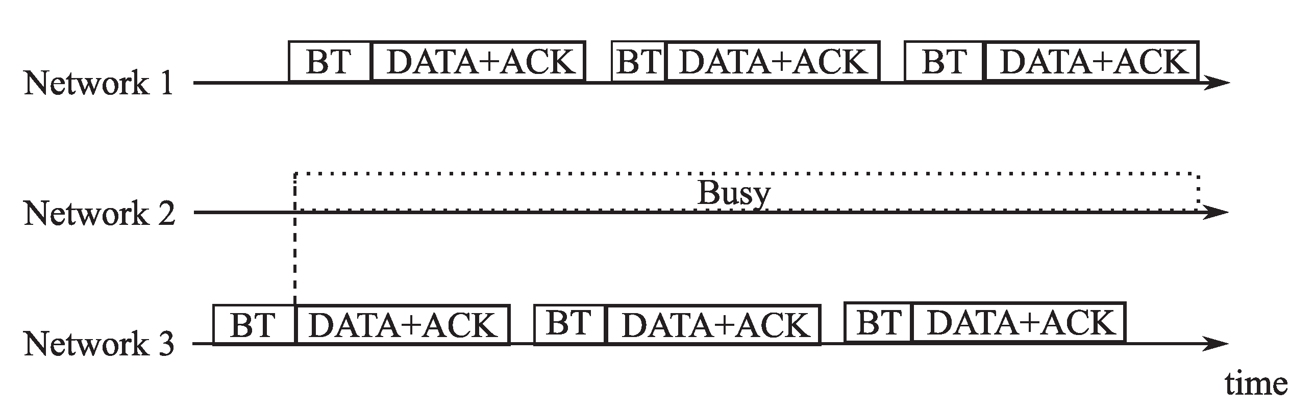
2.2. Inter-Network Interference

As previously mentioned, our considered scenario contains many one-to-one networks, each of which includes an End Device (ED) and the AP. Figure 1 shows an example with three networks. In each WLAN, the distance between the ED and the AP is so close that the neighbor networks are within the ED’s carrier sensing range. There are $E{D}_1$ and $E{D}_3$ in the carrier-sensing range of $E{D}_2$. On the other hand, $E{D}_1$ and $E{D}_3$ have the positional relationship where they cannot detect communication with each other. Therefore, $E{D}_1$ or $E{D}_3$ can transmit when the other is transmitting. $E{D}_2$ cannot decrement the BT because of transmission detection of $E{D}_1$ or $E{D}_3$. It is seen from Figure 2 where transmission opportunity of $E{D}_2$ decreases.

2.3. Motivation to Use Airtime Concept

To properly understand the aforementioned problem, it is essential to consider the interaction of carrier sense. When there is a frame transmission in a network (e.g., Network 1), the other that is out of the carrier-sensing range of Network 1 may also have a transmission. In that case, there is a possibility of having simultaneous transmissions in the networks. It is impossible to get the simultaneous transmission time from the previous analytical models, except the ones with the airtime concept. However, it is difficult to consider that the airtime concept is applied to WLAN analysis because the airtime concept was proposed for expressing the hidden node collisions and carrier-sensing relationships. The analysis of WLANs with airtime concept was proposed in [13], in which the network nodes are assumed to be in saturation and non-saturation heterogeneous conditions. Moreover, the analysis in [14] can express dynamics of various network topologies including multi-hop network and WLANs by using airtime concept. It is also effective to use another extended version of Markov-chain model to express the BT-decrement and frame-transmission states.

However, the analysis in [13] is based on the assumption that there are all nodes in the same carrier-sensing range per one network. Ref. [14] and earlier works [1,2,3,4,5,6,7,8,9,10,11,12,13] have a strict condition that is the main reason for network throughput decreasing is the frame collision. The frame collisions do not occur in the context mentioned in Section 2.2. Therefore, it is necessary to consider the carrier sensing duration. More specifics, the reason of network throughput decreasing is only during the carrier sensing duration. We aim to use the airtime concept to newly express the carrier-sensing duration and the simultaneous transmission time for understanding carrier-sensing duration intuitively.

3. General Concept of Throughput Analysis with Inter-Network Interference

This paper proposes analytical expressions of network throughput for WLANs using the airtime concept with the consideration of inter-network interference. We aim to analytically obtain each network throughput by expressing transmission time, carrier-sensing duration, idle time, and frame-existence probabilities concerning each ED. Our analysis is based on the following assumptions:

• ED in each network generates user datagram protocol (UDP) frames to the AP (uplink) following the Poisson distribution.
• The condition of the physical layer is ideal. Therefore, transmission failures occur due to only frame collisions in the medium access control (MAC) layer.

For better understanding, we show the mathematical symbols of this paper in

Table 1. Mathematical Symbols.

${lim}_{\mathit{T}\mathit{i}\mathit{m}\mathit{e}\to \mathit{\infty }}$	The Limit Value as $\mathit{T}\mathit{i}\mathit{m}\mathit{e}$ Approaches ∞
$S_i$	The transmission duration of Network i in $[0,Time]$
$X_i$	The transmission airtime of Network i
$Y_i$	The carrier-sensing airtime of Network i
$f\left(\right)$	The function to represent $Y_i$
ine $v\left(i\right)$	The set of networks within the carrier-sensing of Network i
$\left|v\right(i\left)\right|$	The number of elements of set $v\left(i\right)$
$h_1,h_2...h_s...h_{\left|v\right(i\left)\right|}$	$h_s$ is the s-th smallest element of $v\left(i\right)$
${\displaystyle \sum _{h\in v\left(i\right)}}$	The sum over all elements h in the set $v\left(i\right)$
${\displaystyle \prod _{h\in v\left(i\right)}}$	The product over all elements h in the set $v\left(i\right)$
$Z_i$	The idle airtime of Network i
$E_i$	The throughput of Network i
P	The payload size of a data frame
T	The period of successful transmission of a data packet
$V_i$	The BT-decrement for one frame-transmission success of Network i
$G_i$	The transmission probability when Network i is in the idle state under the saturation condition
$C{W}_{min}$	The minimum contention-window value
$\sigma$	The slot time
$q_i{}^{\prime }$	The frame-existence probability of Network i in the non-saturation condition
$q_i$	The frame-existence probability of Network i
$O_i$	The offered load of Network i
${\mathsf{\lambda }}_i$	The frame occurrence rate in Network i
${\tau }_i$	The frame transmission probability at the idle state of Network i
${\displaystyle \sum _{\begin{array}{c}k\in v\left(a\right)\cap v\left(b\right)\end{array}}}$	The sum over all elements k in the set $v\left(a\right)\cap v\left(b\right)$
${\displaystyle \prod _{\begin{array}{c}k\in v\left(a\right)\cap v\left(b\right)\end{array}}}$	The product over all elements k in the set $v\left(a\right)\cap v\left(b\right)$
$U_{i,h}$	The probability that Network i is in the idle state when its neighbor Network h is in the idle state
${\gamma }_{i,h}$	The simultaneous transmission probability of Network i and Network h
$v\left(a\right)\cap v\left(b\right)=\left\{5\right\}$	Only Network 5 is within the carrier-sensing range of Network a and b

. Each network node is in one of three states (transmission, carrier-sensing, or idle). The transmission airtime is defined as the time-share of frame transmissions, which includes the duration of both the successful and failed transmissions. Then the transmission airtime of Node i denoted as $X_i$ is as follows:

$$\begin{array}{c}\hfill X_i=\underset{Time\to \infty }{lim}\frac{S_i}{Time},\end{array}$$

(1)

where $S_i$ is the parameter related to the airtime concept for IEEE 802.11, initially introduced in [9]. $S_i$ represents the total duration during which Network i is in the state of DATA frame or ACK frame transmission, SIFS, or DIFS in the time interval of $[0,Time]$.

Because of the carrier-sensing, any transmission within Network i’s carrier-sensing range leads to channel busy. This paper considers the interaction of carrier sensing at each network. Specifically, we examine the overlaps of the multiple transmissions among other networks, which are within the carrier-sensing range of Network i. We use a new function to define $Y_i$, which is the carrier-sensing airtime value (number) of Network i. $Y_i$ can be expressed as

$$\begin{array}{ccc}\hfill Y_i& =& f(X_h,{\gamma }_{i,h}),h\in v\left(i\right)\hfill \\ & =& \sum _{h\in v\left(i\right)}{X}_h(1-{\gamma }_{i,h})-\sum _{h_1<h_2}{X}_{h_1}(1-{\gamma }_{i,h_1})X_{h_2}(1-{\gamma }_{i,h_2})\hfill \\ & +& \sum _{h_1<h_2<h_3}{X}_{h_1}(1-{\gamma }_{i,h_1})X_{h_2}(1-{\gamma }_{i,h_2})X_{h_3}(1-{\gamma }_{i,h_3})-...\hfill \\ & +& {(-1)}^{\left|v\right(i\left)\right|-1}\prod _{\begin{array}{c}h\in v\left(i\right)\end{array}}{X}_h(1-{\gamma }_{i,h}),\hfill \end{array}$$

(2)

where $v\left(i\right)$ is the set of networks within the carrier-sensing of Network i. h is one of the elements in set $v\left(i\right)$. In other word, Network h is in the carrier-sensing range of Network i. $h_s$ in $h_1,h_2...h_s...h_{\left|v\right(i\left)\right|}$ is the s-th smallest element of $v\left(i\right)$. $\left|v\right(i\left)\right|$ is the number of elements of set $v\left(i\right)$. When the back-off timers of both Network i and its adjacent one become zero in the idle state, the two networks will transmit frame simultaneously. The simultaneous transmission probability, in this case, is calculated as ${\gamma }_{i,h}$.

Then the idle airtime of Network i, $Z_i$, is defined as

$$\begin{array}{c}\hfill Z_i=1-X_i-Y_i.\end{array}$$

(3)

Note that $Z_i$ includes the backoff period in the airtime analysis.

Let $E_i$ be the throughput of Network i, then from (1),

$$\begin{array}{c}\hfill {\displaystyle E_i=X_i\frac{P}{T},}\end{array}$$

(4)

T = $DIFS+DATA+SIFS+ACK$ in which $DATA$, $ACK$ are transmission time of only one $DATA$ frame, only one ACK frame, respectively. P is the payload size of a data frame.

According to [21], we also define $G_i$ as the transmission probability when Network i is in the idle state under the saturation condition, then

$$G_i=\frac{R_i}{V_i}=\frac{1}{W_0},$$

(5)

where $R_i$ and $V_i$ are the mean number of frame transmission attempts and the average slot number of BT-decrement for one frame-transmission success, respectively. Additionally, $W_0$ is

$$W_0=C{W}_{min},$$

(6)

where $C{W}_{min}$ is the minimum contention-window value. It is known from [19] that at the saturation condition the relationship between the transmission and idle airtime is

$$X_i=\frac{G_{i}T{Z}_i}{\sigma },$$

(7)

where $\sigma$ is the slot time.

In the non-saturation condition, it is necessary to derive the frame-existence probability $q_i{}^{\prime }$, which is the probability that Network i having at least one frame is in the idle state. Because the BT-decrement is carried out only when the node in the idle state, Network i decreases the BT in whole time is

$$q_i{}^{\prime }{Z}_i={\mathsf{\lambda }}_i\sigma V_i=\frac{\sigma O_i{V}_i}{P},$$

(8)

where $q_i{}^{\prime }$ is the frame-existence probability in the non-saturation condition; ${\mathsf{\lambda }}_i$ is the frame occurrence rate; $O_i={\mathsf{\lambda }}_{i}P$ is the offered load. Additionally, $\sigma V_i$ means the average time of BT-decrement for one successful transmission of a frame. (8) is based on the fact that the frame-occurrence number same as the frame-transmission number in the non-saturation condition.

From (8), it is possible to express the frame-existence probability $q_i$ as

$$\begin{array}{c}\hfill q_i=\left\{\begin{array}{cc}{q}_i{}^{\prime },\hfill & non-saturation\hfill \\ 1,\hfill & saturation\hfill \end{array}\right.\end{array}$$

(9)

Because of $q_i{}^{\prime }<1$ from its definition, it can be rewritten as

$$q_i=min\left(1,q_i{}^{\prime }\right)=min\left(1,\frac{\sigma O_i{V}_i}{P{Z}_i}\right),$$

(10)

which is valid for both the saturation and non-saturation states. The min function prevents $q_i$ from exceeding 1. By using ${\mathsf{\lambda }}_i$, we have also another expression of transmission airtime as

$$X_i={\mathsf{\lambda }}_i{R}_{i}T.$$

(11)

From (5), (8), and (11), we have

$$X_i=\frac{q_i{Z}_i{G}_{i}T}{\sigma }.$$

(12)

Finally, the general expression of the frame transmission probability at the idle state (denoted as ${\tau }_i$) can be obtained from (7), (10) and (11) as

$${\tau }_i=q_i{G}_i=\frac{\sigma X_i}{Z_{i}T}.$$

(13)

The derivation and explanation of the Equations (5)–(13) have been also presented in [11,12,13,14].

Our analysis aims to consider the channel states of each network. From (2), we use $v\left(i\right)$ to denote the set of networks within the carrier-sensing of Network i, and Network h indicates the element of a set $v\left(i\right)$. Network i is in the idle state or the carrier-sensing state when its adjacent network (e.g., Network h) can decrement back-off timer. When Network h is in the idle state, the probability $U_{i,h}$ that the state of Network i in the idle state is

$$\begin{array}{c}\hfill U_{i,h}=1-f(X_j,{\gamma }_{i,j});j\ne h;j,h\in v\left(i\right).\end{array}$$

(14)

When the back-off timers of both Network i and its adjacent one become zero in the idle state, the two networks will transmit frame simultaneously. Let ${\gamma }_{i,h}$ be the simultaneous transmission probability in this case. Then, we have

$$\begin{array}{c}\hfill {\displaystyle {\gamma }_{i,h}=U_{i,h}·{\tau }_i,}\end{array}$$

(15)

where ${\tau }_i$ is the frame transmission probability at the idle state, h is the elements in the set $v\left(i\right)$.

4. Throughput Analysis of String and Grid Topology Considering Inter-Network Interference

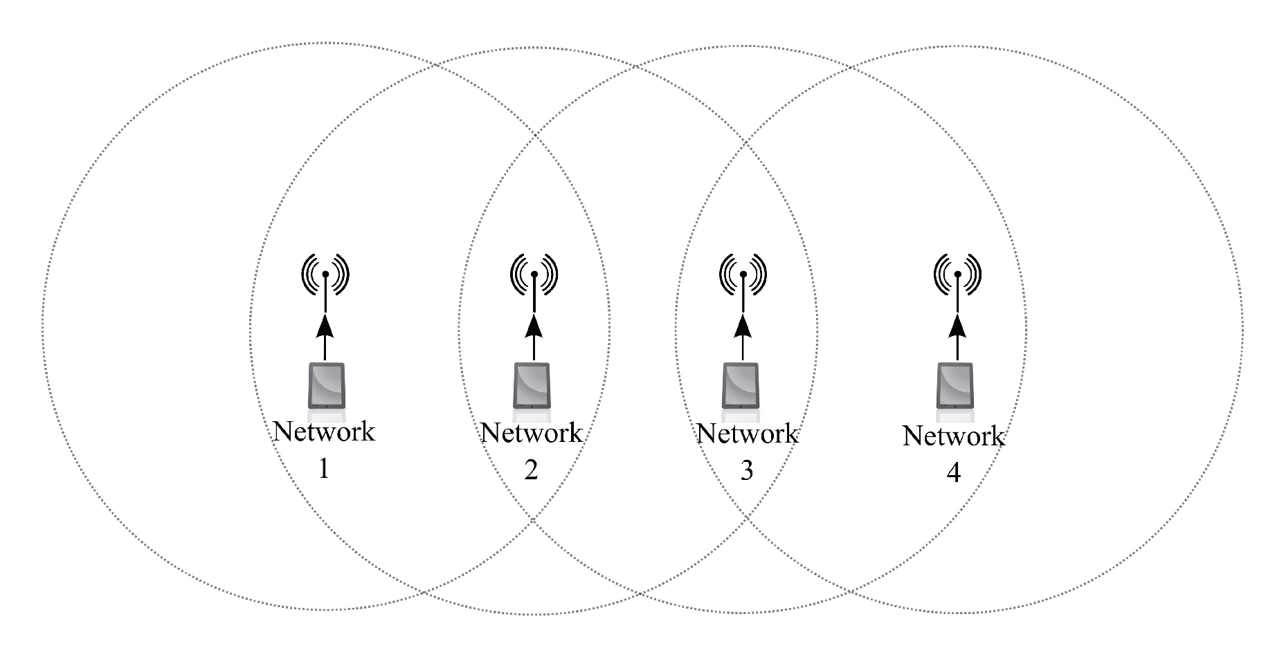
4.1. Analysis of String Network Topology

In a 1 × n string topology as in Figure 3, only one network is within the carrier-sensing range of the leftmost or rightmost network. When an adjacent network of the leftmost one is in the idle state, the network does not have a carrier sensing or transmission events. Hence, the probability of the leftmost network in the idle state is 1. That happens similarly to the rightmost network. Except for those cases, Network $(i-1)$ and Network $(i+1)$ are within carrier-sensing range of Network i. Hence, at Network i, the carrier-sensing network number is two.

From (14), assume that Network $(i-1)$ is in the idle state, Network i is never in the transmission state. Therefore, there will be two possibilities of Network i’s state: idle or carrier-sensing. The carrier-sensing state of Network i can be caused by the transmission of either Network $(i-1)$ or Network $(i+1)$. That is because the two networks are in the carrier-sensing range of Network i in the string topology. However, we have assumed that Network $(i-1)$ is in the idle state; therefore, the carrier-sensing state of Network i is only caused by the transmission state of Network $(i+1)$. The accurate expression of the probability can be

$$\begin{array}{c}\hfill U_{i,i-1}=1-\frac{X_{i+1}}{1-X_i}.\end{array}$$

(16)

$U_{i,i+1}$ is the probability that the state of Network i is in the idle state, when Network $(i-1)$ is in the idle state. It can be derived in the similar way.

The carrier-sensing airtime is the time-share when the network is in the carrier-sensing state. Basically, the carrier-sense airtime of Network i is the total transmission airtime of the carrier-sensing nodes. From (2), the carrier-sensing airtime of Network i could be obtained accurately.

$$\begin{array}{ccc}\hfill Y_i& =& X_{i-1}(1-{\gamma }_{i,i-1})+X_{i+1}(1-{\gamma }_{i,i+1})\hfill \\ & -& \frac{X_{i-1}(1-{\gamma }_{i,i-1})X_{i+1}(1-{\gamma }_{i,i+1})}{1-X_i}.\hfill \end{array}$$

(17)

Note that, $X_{i-1}$ and $X_{i+1}$ equal to 0 when Network i is the leftmost, rightmost network, respectively. The final component in the right-hand side of (17) denotes the overlap time between Network $(i-1)$ and $(i+1)$ when Network i does not transmit.

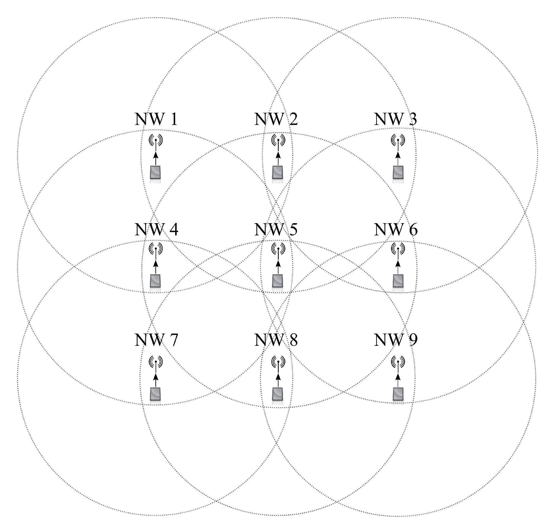
4.2. Analysis of Grid Network Topology

In the grid topology, depending on a network position, the number of networks within the carrier-sensing range is different. Therefore, it is necessary to consider the carrier-sensing airtime and the simultaneous transmission time following the network number in the carrier-sensing range. If Network i is in the m × n grid network topology, the network number could be two, three, and four. For the sake of easy presentation, this section investigates the case of m = n = 3. With the other values of m, n, we can similarly deduce each network state.

4.2.1. Two Carrier-Sensing Networks

As shown in Figure 4, in the investigated topology, Network 1, 3, 7, and 9 are in accord with this case. Since the four networks share the same characteristics, we consider only Network 1 in the following. From (14), when the state of Network 2 is idle, the probability of Network 1 being in the idle state can be expressed as in (18).

$$\begin{array}{ccc}{U}_{1,a}\hfill & =\hfill & 1-\frac{X_b}{1-{\displaystyle \sum _{\begin{array}{c}k\in v\left(a\right)\cap v\left(b\right)\end{array}}}\left[X_k{\displaystyle \prod _{\begin{array}{c}h\in v\left(k\right)\end{array}}}(1-{\gamma }_{h,k})\right]+{\displaystyle \prod _{\begin{array}{c}k\in v\left(a\right)\cap v\left(b\right)\end{array}}}\left[X_k{\displaystyle \prod _{\begin{array}{c}h\in v\left(k\right)\end{array}}}(1-{\gamma }_{h,k})\right]{(1-Y_1)}^{-1}};\hfill \\ \hfill & \hfill & a,b\in v\left(1\right),a\ne b.\hfill \end{array}$$

(18)

We use $v\left(i\right)$ to denote the set of networks within the carrier-sensing of Network i, which is the same as the following, such as $v\left(a\right)$, $v\left(b\right)$, $v\left(k\right)$ and so on. ${\displaystyle \prod _{\begin{array}{c}k\in v\left(a\right)\cap v\left(b\right)\end{array}}}\left[X_k{\displaystyle \prod _{\begin{array}{c}h\in v\left(k\right)\end{array}}}(1-{\gamma }_{h,k})\right]{(1-Y_1)}^{-1}$ is the overlap transmitting time between Network 1 and 5.

Network 2 and Network 4 is in the carrier-sensing range of Network 1. From (2), the carrier-sensing airtime of Network 1 can be transformed as (19).

$$\begin{array}{ccc}\hfill Y_1& =& {\displaystyle \sum _{i\in v\left(1\right)}}{X}_i(1-{\gamma }_{1,i})\hfill \\ & -& \frac{{\displaystyle \prod _{\begin{array}{c}i\in v\left(1\right)\end{array}}}{X}_i(1-{\gamma }_{1,i})}{1-{\displaystyle \sum _{k\in v\left(i\right)}}\left[X_k{\displaystyle \prod _{\begin{array}{c}h\in v\left(k\right)\end{array}}}(1-{\gamma }_{h,k})\right]+{\displaystyle \prod _{k\in v\left(i\right)}}\left[X_k{\displaystyle \prod _{\begin{array}{c}h\in v\left(k\right)\end{array}}}(1-{\gamma }_{h,k})\right]{(1-Y_1)}^{-1}}.\hfill \end{array}$$

(19)

The final member of the right-hand side denotes the overlap transmitting time between Network 2 and 4 when Network 1 and 5 do not transmit.

4.2.2. Three Carrier-Sensing Networks

As shown in Figure 4, Network 2, 4, 6 and 8 are in accord with this case. Due to the position similarity, we only consider Network 2. In this case, $v\left(2\right)$ includes Network 1, 3, 5. Hence, when a ≠ 5, the probability of Network 2 being in the idle state is

$$\begin{array}{ccc}\hfill U_{2,a}& =& 1-\frac{X_b}{1-X_2}-\frac{X_5}{1-Y_a}+\frac{X_b{X}_5}{(1-Y_a)(1-Y_b)};\hfill \\ & & a,b\in v\left(2\right),a\ne b,b\ne 5.\hfill \end{array}$$

(20)

We know Network 2 is within Network a and Network b’s carrier-sensing range. Because Network 2 does not transmit, the probability of Network b transmitting in this condition is $\frac{X_b}{1-X_2}$. Network 2 and one other (Network c) are within the carrier-sensing range of Network a and Network 5. When Network 2 and Network a are in the idle state, Network c does not transmit either. In this case, the probability $\frac{X_5}{1-X_2-X_c}$ is not enough, because of considering the simultaneous transmission time of Network a and Network 5. The correct expression is $\frac{X_5}{1-Y_a}$. The final component of the right-hand side in (20) denotes the overlap time between Network b and Network 5. When a = 5, $U_{2,5}$ is

$$\begin{array}{ccc}\hfill U_{2,5}& =& 1-\frac{X_1}{1-Y_1}-\frac{X_3}{1-Y_3}+\frac{X_1{X}_3}{(1-Y_1)(1-Y_3)}.\hfill \end{array}$$

(21)

Similar to in (20), the rightmost component of (21) shows the probability of overlap time between Network 1 and Network 3. We know Network $\left\{2,4\right\}$, Network $\left\{2,6\right\}$ are within the carrier-sensing range of Network $\left\{1,5\right\}$, Network $\left\{3,5\right\}$, respectively. In the former condition, the probability of Network 5 transmitting is $\frac{X_1}{1-Y_1}$. In the latter, the probability is $\frac{X_3}{1-Y_5}$.

From (2) we derive the carrier-sensing airtime of Network 2 as follows.

$$\begin{array}{ccc}\hfill Y_2& =& \sum _{i\in v\left(2\right)}{X}_i(1-{\gamma }_{2,i})-\frac{{\displaystyle \prod _{\begin{array}{c}k\in v\left(2\right)\\ k\ne 5\end{array}}}{X}_k(1-{\gamma }_{2,k})}{1-X_2}\hfill \\ & -& {\displaystyle \sum _{\begin{array}{c}k\in v\left(2\right)\\ k\ne 5\end{array}}}\frac{X_k(1-{\gamma }_{2,k})X_5(1-{\gamma }_{2,5})}{1-Y_k}+{\displaystyle \prod _{\begin{array}{c}i\in v\left(2\right)\end{array}}}\frac{X_i(1-{\gamma }_{2,i})}{(1-Y_i)}.\hfill \end{array}$$

(22)

In (22) the simultaneous time of Network 1 and Network 3 is $\frac{{\displaystyle \prod _{\begin{array}{c}k\in v\left(2\right)\\ k\ne 5\end{array}}}{X}_k(1-{\gamma }_{2,k})}{1-X_2}$, because in such condition there is no transmission in Network 2. Because of no transmission in Network $\left\{2,4\right\}$ and Network $\left\{2,6\right\}$, the simultaneous time of Network 1 (or Network 3) and Network 5 can be expressed as $\frac{X_k(1-{\gamma }_{2,k})X_5(1-{\gamma }_{2,5})}{1-Y_k}$. The last line in (22) denotes the overlap time between Network 1, Network 3, and Network 5.

4.2.3. Four Carrier-Sensing Networks

As shown in Figure 4, Network 5 is in accord with this case. There are Network $\left\{2,4,6,8\right\}$ within carrier-sensing range of Network 5. From (14), the probability that the state of Network 5 is idle can be expressed as (23). $v\left(a\right)\cap v\left(b\right)=\left\{5\right\}$ means only Network 5 is within the carrier-sensing range of Network $\left\{a,b\right\}$. We can see the pairs of Network $\left\{2,8\right\}$, or Network $\left\{4,6\right\}$ meet this condition. Moreover, when $\left\{a,b\right\}$ is $\left\{2,8\right\}$ then Network c is only Network 4 or Network 6, and vice versa.

$$\begin{array}{ccc}{U}_{5,a}\hfill & =\hfill & 1-\sum \frac{X_c}{1-{\displaystyle \sum _{\begin{array}{c}k\in v\left(a\right)\cap v\left(b\right)\end{array}}}\left[X_k{\displaystyle \prod _{\begin{array}{c}h\in v\left(k\right)\end{array}}}(1-{\gamma }_{h,k})\right]+{\displaystyle \prod _{\begin{array}{c}k\in v\left(a\right)\cap v\left(b\right)\end{array}}}\left[X_k{\displaystyle \prod _{\begin{array}{c}h\in v\left(k\right)\end{array}}}(1-{\gamma }_{h,k})\right]{(1-Y_m)}^{-1}}\hfill \\ \hfill & -\hfill & \frac{X_b}{1-Y_a{Y}_b}+\frac{\prod X_c}{(1-\prod Y_c)(1-Y_a)}+\sum \frac{X_b{X}_c}{(1-Y_a{Y}_b)(1-Y_c)}-\frac{{\displaystyle \prod _{\begin{array}{c}l\in v\left(5\right)\\ l\ne a\end{array}}}{X}_l(1-{\gamma }_{5,l})}{(1-Y_a{Y}_b)\prod (1-Y_c)};\hfill \\ \hfill & \hfill & v\left(a\right)\cap v\left(b\right)=\left\{5\right\},c\in v\left(5\right),a\ne b,b\ne c,a\ne c,m=k,m\ne 5.\hfill \end{array}$$

(23)

For the easy presentation, we explain the value of the second component in (23) in the case of $a=2$. Network $\left\{5,7,9\right\}$ are within Network 8’s carrier-sensing range. Moreover, Network 2 and Network 8 are in the carrier-sensing state when Network 5 does not transmit. That can be expressed $(1-Y_2{Y}_8)$. The probability of Network 8 transmitting in this condition is $\frac{X_8}{1-Y_2{Y}_8}$. The probability of Network c simultaneous transmitting can be expressed as $\frac{X_4{X}_6}{(1-Y_4{Y}_6)(1-Y_2)}$ in the forth component in (23), because c equals 4 or 6. We consider the relationship of Network 2 and Network $\left\{4,6\right\}$. From that, we can know Network $\left\{1,3,5\right\}$ are in the carrier-sensing range of Network $\left\{2,4,6\right\}$. In this condition, $(1-Y_4{Y}_6)$ means Network 5 does not transmit. $(1-Y_4{Y}_6)(1-Y_2$) means Network $\left\{1,3,5\right\}$ do not transmit. Other components are calculated similarly as the ones in the previous sections. We can express $U_{5,4}$,$U_{5,6}$, and $U_{5,8}$ using the similar method.

From (2), the carrier-sensing airtime of Network i could be obtained accurately in (24).

$$\begin{array}{ccc}\hfill Y_5& =& \sum _{i\in v\left(5\right)}{X}_i(1-{\gamma }_{5,i})\hfill \\ & -& \sum _{j\notin v\left(5\right)}\frac{{\displaystyle \prod _{\begin{array}{c}l\in v\left(j\right)\end{array}}}{X}_l(1-{\gamma }_{5,l})}{1-{\displaystyle \sum _{k\in v\left(l\right)}}\left[X_k{\displaystyle \prod _{\begin{array}{c}h\in v\left(k\right)\end{array}}}(1-{\gamma }_{h,k})\right]+{\displaystyle \prod _{k\in v\left(l\right)}}\left[X_k{\displaystyle \prod _{\begin{array}{c}h\in v\left(k\right)\end{array}}}(1-{\gamma }_{h,k})\right]{(1-Y_j)}^{-1}}\hfill \\ & -& \sum \frac{X_a(1-{\gamma }_{5,a})X_b(1-{\gamma }_{5,b})}{1-Y_a{Y}_b}+\sum \frac{X_a(1-{\gamma }_{5,a})X_b(1-{\gamma }_{5,b})X_c(1-{\gamma }_{5,c})}{(1-Y_a{Y}_b)(1-Y_c)}\hfill \\ & -& \frac{{\displaystyle \prod _{\begin{array}{c}i\in v\left(5\right)\end{array}}}{X}_i(1-{\gamma }_{5,i})}{(1-Y_a{Y}_b)\prod (1-Y_c)};v\left(a\right)\cap v\left(b\right)=\left\{5\right\},c\in v\left(5\right),a\ne b,b\ne c,a\ne c.\hfill \end{array}$$

(24)

Specifically, when Network a and Network b transmit simultaneously, only Network 5 is within their carrier-sensing ranges, and we know Network 5 does not have transmission. In (24), ($1-Y_a{Y}_b$) means Network 5 does not transmit in this condition. Therefore, the simultaneous transmission time of Network a and Network b is $\frac{X_a(1-{\gamma }_{5,a})X_b(1-{\gamma }_{5,b})}{1-Y_a{Y}_b}$. In the case of three networks, for example, Network $\left\{a,b,c\right\}$ transmit simultaneously. When a = 2; b = 4; c = 6, Network $\left\{1,3,5\right\}$ are within the carrier-sensing range of Network $\left\{a,b,c\right\}$. $(1-Y_2)$ means Network 1 and 3 do not transmit. $(1-Y_4{Y}_8)$ presents the condition of Network 5 without transmission. $(1-Y_4{Y}_8)$ presents the condition of Network 5 without transmission. Therefore, the simultaneous transmission time of Network $\left\{2,4,6\right\}$ is $\frac{X_2(1-{\gamma }_{5,2})X_4(1-{\gamma }_{5,4})X_6(1-{\gamma }_{5,6})}{(1-Y_4{Y}_6)(1-Y_2)}$. Using the similar method, the simultaneous transmission time of Network Network $\left\{a,b,c\right\}$ is $\frac{X_a(1-{\gamma }_{5,a})X_b(1-{\gamma }_{5,b})X_c(1-{\gamma }_{5,c})}{(1-Y_a{Y}_b)(1-Y_c)}$. Other components are calculated similarly as the ones in the previous sections.

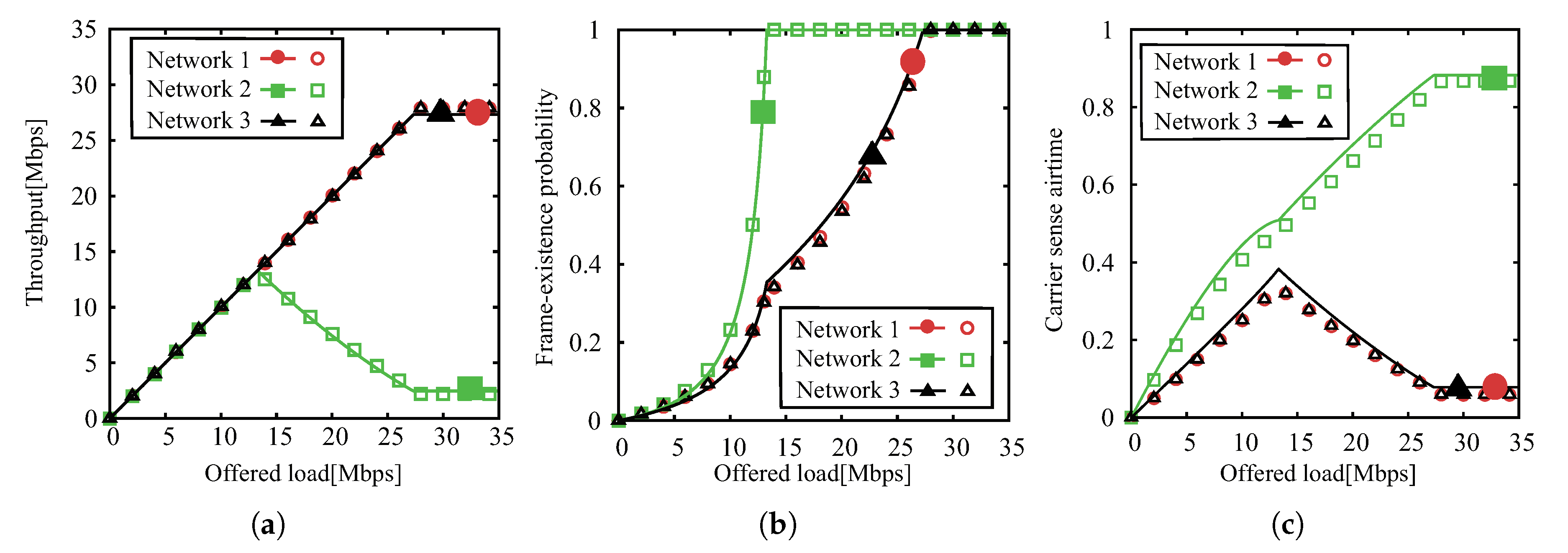
5. Performance Evaluation

For showing the validity of the analytical expressions, in the previous section, we compare the analytical results with the simulation ones in this section. The simulator is our in-house implementation, in which the wireless networks operate following the IEEE 802.11 standard. Note that our simulator has been efficiently applied in several previous works [11,12,13,14,15,16,17]. Moreover, we have published the simulator’s source codes on the website in [23].

Table 2. System Parameters.

Data payload	1500 bytes
PHY header	24 bytes
MAC header	24 bytes
ACK size	10 bytes
Data rate	54 Mbps
ACK bit rate	24 Mbps
DATA	$252\mathsf{\mu }s$
DIFS	$34\mathsf{\mu }s$
SIFS	$16\mathsf{\mu }s$
Slot time ($\sigma$)	$9\mathsf{\mu }s$
$C{W}_{min}$	15
$C{W}_{max}$	1023
Retry limit (K)	7
Inter-network distance	30 m
Transmission range	40 m
Carrier-sensing range	40 m

gives system parameters, which are used in the simulations and analytical predictions. The parameters basically follow the IEEE 802.11a standard. Each inter-network’s distance is 30 m.

5.1. Scenario 1: String Topology, $N=3$

In Scenario 1, there are three networks which are installed linearly. Figure 5a–c show the network performance as a function of the offered load. It is seen from Figure 5a that the throughput increases in proportion to the offered load in the range of $0\le O\le 13.3$ Mbps. This is because all the networks are in the non-saturation state. The observation is confirmed from Figure 5b, where we can see that frame-existence probabilities of all the nodes are less than one in the range. The frame-existence probability of Network 2 reaches one first at $O=13.3$ Mbps. For $O\ge 13.3$ Mbps, the frame-existence probabilities of networks except Network 2 still increase. It leads to the increment of the carrier-sensing probabilities, which are confirmed from Figure 5c. As a result, the throughput of Network 2 decreases as the offered load increases in the saturation condition. It is also seen from Figure 5b that all networks are saturated when $O=28.1$ Mbps. Therefore, the network throughput with respect to each network keeps the constant value in the range of $O\ge 28.1$ Mbps. From Figure 5c, it is confirmed that the degradation of throughput in Network 2 is caused by the bias of carrier-sensing.

5.2. Scenario 2: String Topology, $N=4$

Scenario 2 includes four linear networks. Figure 6a–c show the network throughput, frame-existence probability, carrier-sense airtime, as functions of offered load, respectively. We can observe from Figure 6a that the throughputs increase in proportion to the offered load in the range of $0\le O\le 13.3$ Mbps. The reason is similar to the one in the previous section (i.e., networks being in the non-saturation state). We also have same confirmation as in Figure 6b, where within the range all the probabilities are less than one. However, the frame-existence probabilities of Network 2 and 3 reach one at $O=13.2$ Mbps. For $O\ge 13.2$ Mbps, meanwhile the frame-existence probabilities of the other networks still increase. Therefore, carrier-sensing probabilities increase as seen in Figure 6c. As a result, the throughputs of Network 2 and 3 decrease as the offered load increases in the saturation condition. It is also seen from Figure 6b that all networks are saturated at $O=20.5$ Mbps. Therefore, the network throughputs keep the constant value in the range of $O\ge 20.5$ Mbps. From Figure 6c, it is confirmed that the degradation of throughput in Network 2 and 3 is also caused by the bias of carrier-sensing.

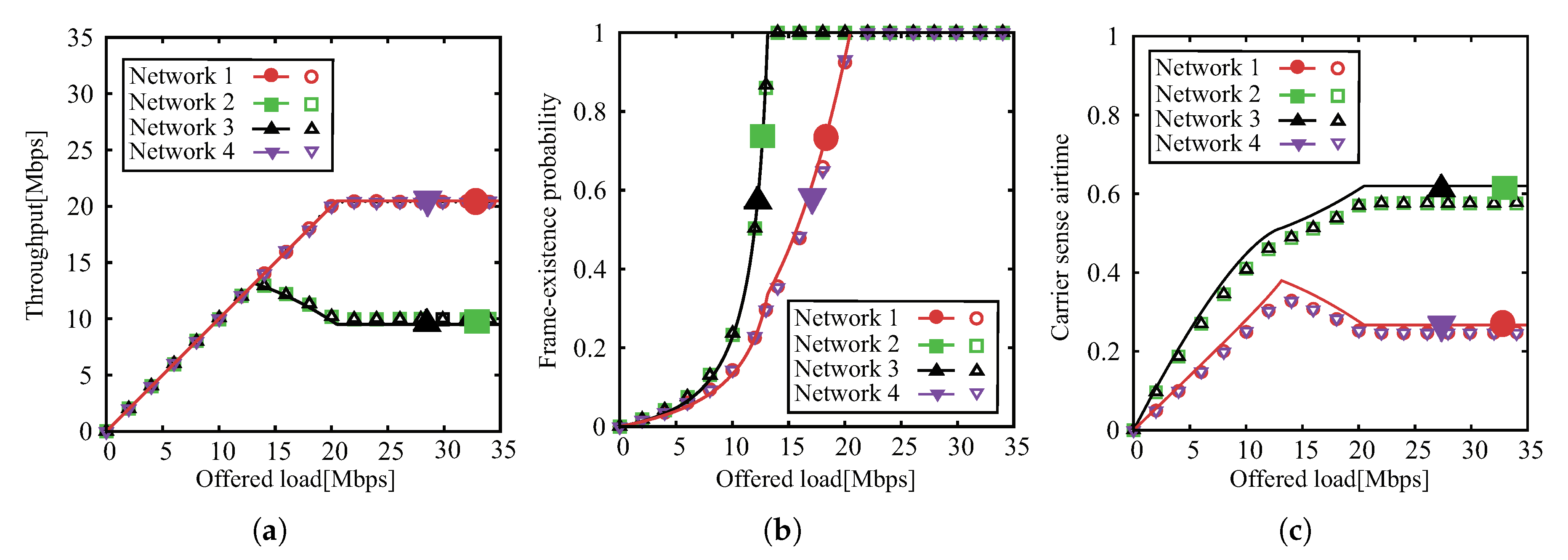
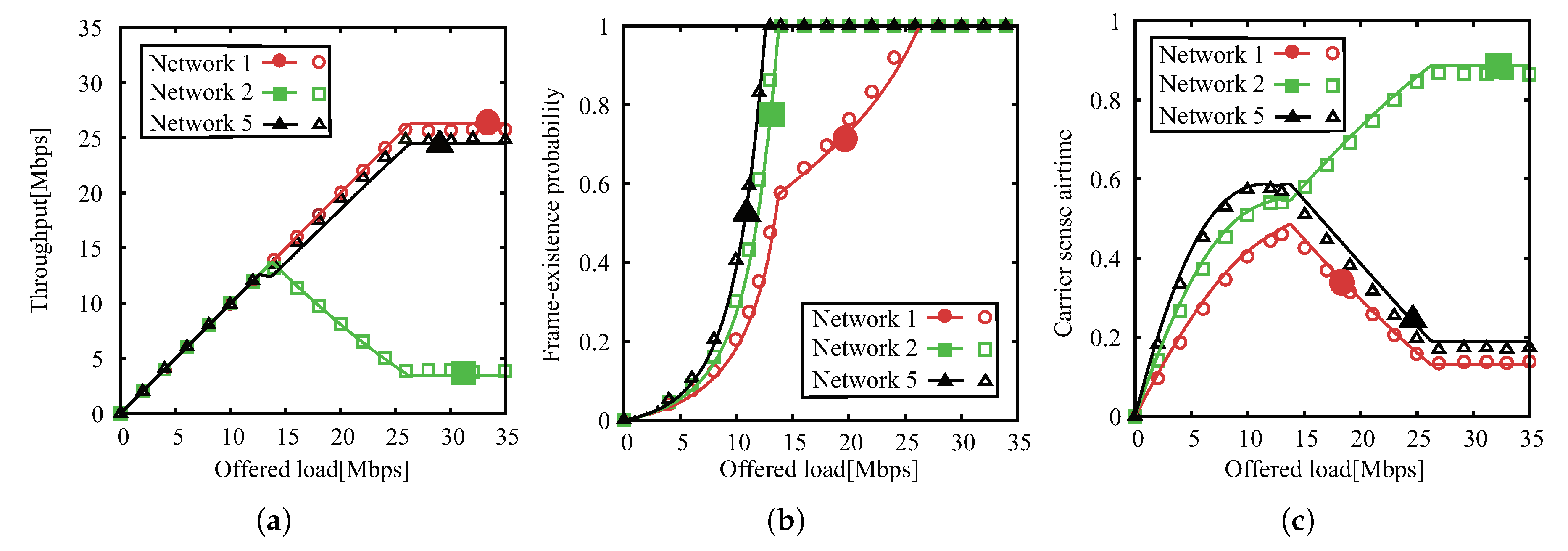
5.3. Scenario 3: Grid Topology

In Scenario 3, there are nine networks installed in a grid shape. Figure 7a–c show the network performance as a function of offered load. Figure 7a shows that similar to the string topologies the throughputs increase in proportion to the offered load in the range of $0\le O\le 13.6$ Mbps. Within that range, the frame-existence probabilities of all the nodes are less than one because all the networks are in non-saturation state as in Figure 7b. In this case, the frame-existence probability of Network 2 reaches one at $O=12.75$ Mbps, and Network 5 reaches one at $O=13.6$ Mbps. However, the throughput of Network 5 continues to increase as the offered load increases although the frame-existence probability of Network 5 reaches one at $O=13.6$ Mbps. Because Network 2 loses the transmission opportunities when the offered load increases, Network 5 gets the transmission opportunities. For $O\ge 13.6$ Mbps, the frame-existence probabilities of networks except Network 2 and 5 still increase. Therefore, the carrier-sensing probabilities increase, which can be confirmed from Figure 7c. As a result, the throughput of Network 2 decreases as offered load increases in the saturation condition. It is also seen from Figure 7b that all networks are saturated at $O=26.0$ Mbps. From Figure 7c, it is confirmed that the degradation of throughput in Network 2 is also caused by bias of carrier-sensing. However, we observe the throughput of Network 5 does not increase markedly at $12.75$ Mbps $\le O\le$$13.6$ Mbps. Because the frame-existence probability of Network 5 reaches one at $O=12.75$ Mbps first. It is faster than Network 2. The carrier sensing duration of Network 5 decreases and Network 2 increases at $O=11.8$ Mbps. Although the frame-existence probability of Network 5 reaches one first, Network 5 gets more the transmission opportunities at $O=11.8$ Mbps. When the frame-existence probability of Network 2 reaches one at $O=13.6$ Mbps, the throughput of Network 5 increases markedly.

It is seen that in all the Figure 5, Figure 6 and Figure 7 the analytical predictions well agree with the simulation results. That confirms the validities of the analytical expressions in this work. Not only that the results in all the scenarios show the large variation of network throughput caused by the carrier-sensing effect. Therefore, our findings can provide a convenient tool to understand the variation.

6. Conclusions

This paper has proposed the analytical expressions of one-to-one WLAN’s throughput under the impact of inter-network interference. The analysis, which uses the airtime concept, can provide each network throughput by expressing the simultaneous transmission time, carrier-sensing duration, and frame-existence probabilities concerning each network. We have applied the analytical expressions in three scenarios, including the two string topologies and a grid one. The validity of the analytical expressions has been confirmed from the quantitative agreements between the analytical and simulation results.

References

1. Bianchi, G. Performance analysis of IEEE 802.11 distributed coordination function. Proc. IEEE J. Sel. Areas Commun. 2000, 18, 535–547. [Google Scholar] [CrossRef]
2. Duffy, K.; Malone, D.; Leith, D. Modeling the 802.11 distributed coordination function in nonsaturared conditions. IEEE Commun. Lett. 2005, 9, 715–717. [Google Scholar] [CrossRef]
3. Zhang, H.; Zhang, X.; Chen, G. Performance analysis of IEEE802.11 DCF in non-saturated conditions. In Proceedings of the 2011 International Conference on Business Management and Electronic Information, Guangzhou, China, 13–15 May 2011; pp. 495–498. [Google Scholar]
4. Kim, T.; Lim, J.T. Throughput analysis considering coupling effect in IEEE 802.11 networks with hidden stations. IEEE Commun. Lett. 2009, 13, 175–177. [Google Scholar] [CrossRef]
5. Qin, Z.; Xiao, J.; Xie, H. A novel model for non-saturated performance analysis of IEEE802.11 DCF. In Proceedings of the 2012 2nd International Conference on Consumer Electronics, Communications and Networks (CECNet), Yichang, China, 21–23 April 2012; pp. 1552–1556. [Google Scholar]
6. Iwami, T.; Takaki, Y.; Yamori, K.; Ohta, C.; Tamaki, H. Distributed association control considering user utility and user guidance in IEEE802.11 networks. In Proceedings of the 2013 IEEE 24th Annual International Symposium on Personal, Indoor, and Mobile Radio Communications (PIMRC), London, UK, 8–11 September 2013; pp. 2125–2130. [Google Scholar]
7. Deng, X.; He, T.; He, L.; Gui, J.; Peng, Q. Performance analysis for IEEE 802.11s wireless mesh network in smart grid. Wirel. Pers. Commun. 2017, 96, 1537–1555. [Google Scholar] [CrossRef]
8. Li, X.; Narita, Y.; Gotoh, Y.; Shioda, S. Performance analysis of IEEE 802.11 DCF based on a macroscopic state description. IEICE Trans. Commun. 2018, E101-B, 1923–1932. [Google Scholar] [CrossRef]
9. Ng, P.C.; Liew, S.C. Throughput analysis of IEEE 802.11 multi-hop ad hoc networks. IEEE/ACM Trans. Netw. 2007, 15, 309–322. [Google Scholar] [CrossRef]
10. Barowski, Y.D.; Biaz, S.; Agrawal, P. Towards the performance analysis of IEEE 802.11 in multi-hop ad-hoc networks. In Proceedings of the WCNC, New Orleans, LA, USA, 13–17 March 2005; Volume 1, pp. 100–106. [Google Scholar]
11. Shimoyamada, Y.; Sanada, K.; Komuro, N.; Sekiya, H. End-to-end throughput analysis for IEEE 802.11e EDCA string-topology wireless multi-hop networks. Nonlinear Theory Its Appl. 2015, E6-N, 410–432. [Google Scholar] [CrossRef] [Green Version]
12. Sanada, K.; Shi, J.; Komuro, N.; Sekiya, H. End-to-end delay analysis for IEEE 802.11 string-topology multi-hop networks. IEICE Trans. Commun. 2015, E98-B, 1284–1293. [Google Scholar] [CrossRef] [Green Version]
13. Wan, Y.; Sanada, K.; Komuro, N.; Motoyoshi, G.; Yamagaki, N.; Shioda, S.; Sakata, S.; Murase, T.; Sekiya, H. Throughput analysis of WLANs in saturation and non-saturation heterogeneous conditions with airtime concept. IEICE Trans. Commun. 2016, E99-B, 2289–2296. [Google Scholar] [CrossRef] [Green Version]
14. Sanada, K.; Sekiya, H. Bottom-up analysis concept for throughput and delay analyses of wireless network. Nonlinear Theory Its Appl. 2017, 8, 181–203. [Google Scholar] [CrossRef] [Green Version]
15. So, J.; Lee, J. Dynamic carrier-sense threshold selection for improving spatial reuse in dense Wireless LANs. Appl. Sci. 2019, 9, 3951. [Google Scholar] [CrossRef] [Green Version]
16. Kanematsu, T.; Nguyen, K.; Sekiya, H. Throughput analysis for IEEE 802.11 multi-Hop networks considering transmission rate. In Proceedings of the IEEE VTC Spring 2019, Kuala Lumpur, Malaysia, 28 April–1 May 2019; pp. 1–5. [Google Scholar]
17. Ikuma, S.; Li, Z.; Pei, T.; Choi, Y.; Sekiya, H. Rigorous analytical model of saturated throughput for the IEEE 802.11p EDCA. IEICE Trans. Commun. 2019, E102-B, 699–707. [Google Scholar] [CrossRef]
18. Kelley, C.T. Iterative Methods for Linear and Nonlinear Equations; North Carolina State University: Raleigh, NC, USA, 1995. [Google Scholar]
19. Gao, Y.; Chui, D.; Lui, J.C.S. Determining the end-to-end throughput capacity in multi-hop networks: Methodology applications. In Proceedings of the SIGMETRICS/Performance 2006, Saint Malo, France, 26–30 June 2006; pp. 39–50. [Google Scholar]
20. Inaba, M.; Tsuchiya, Y.; Sekiya, H.; Sakata, S.; Yagyu, K. Analysis and experiments of maximum throughput in wireless multi-hop networks for VoIP application. IEICE Trans. Commun. 2009, E92-B, 3422–3431. [Google Scholar] [CrossRef] [Green Version]
21. Kumar, A.; Altman, E.; Miorandi, D.; Goyal, M. New insights from a fixed point analysis of single cell IEEE 802.11 Wireless LANs. IEEE/ACM Trans. Netw. 2007, 15, 588–600. [Google Scholar] [CrossRef] [Green Version]
22. Wireless LAN Medium Access Control (MAC) and Physical Layer (PHY) Specifications; IEEE Std. 802.11; IEEE: Piscataway, NJ, USA, 2012.
23. The Simulator’s Source Code. Available online: http://www.s-lab.nd.chiba-u.jp/link/simulator.htm (accessed on 24 January 2020).
Figure 1. Scenario with inter-network interference.
Applsci 10 02192 g001
Figure 2. An exemplary effect of inter-network interference.
Applsci 10 02192 g002
Figure 3. Carrier-sensing range of each network in string-topology.
Applsci 10 02192 g003
Figure 4. Carrier-sensing range of each network in grid-topology.
Applsci 10 02192 g004
Figure 5. Network characteristics of analytical (lines) and simulation (plots) results as a function of the offered load for Scenario 1. (a) Throughput. (b) Frame-existence probability. (c) Carrier-sense airtime.
Applsci 10 02192 g005
Figure 6. Network characteristics of analytical (lines) and simulation (plots) results as a function of the offered load for Scenario 2. (a) Throughput. (b) Frame-existence probability. (c) Carrier-sense airtime.
Applsci 10 02192 g006
Figure 7. Network characteristics of analytical (lines) and simulation (plots) results as a function of the offered load for Scenario 3. (a) Throughput. (b) Frame-existence probability. (c) Carrier-sense airtime.
Applsci 10 02192 g007