Microseismic Signal Denoising via Empirical Mode Decomposition, Compressed Sensing, and Soft-thresholding

Abstract

Microseismic signal denoising is of great significance for P wave, S wave first arrival picking, source localization, and focal mechanism inversion. Therefore, an Empirical Mode Decomposition (EMD), Compressed Sensing (CS), and Soft-thresholding (ST) combined EMD_CS_ST denoising method is proposed. First, through EMD decomposition of the noise signal, a series of Intrinsic Mode Functions (IMF) from high frequency to low frequency are obtained. By calculating the correlation coefficient between each IMF and the original signal, the boundary component between the signal and the noise was identified, and the boundary component and its previous components were sparsely processed in the discrete wavelet transform domain to obtain the original sparse coefficient θ. Second, θ is filtered by ST to get the reconstruction coefficient θ_new after denoising. Then, CS was used to recover and reconstruct θ_new to get the denoised IMF_new component and then recombined with the remaining IMF components to get the signal after denoising. In the simulation experiment, the denoising process of EMD_CS_ST method is introduced in detail, and the denoising ability of EMD_CS_ST, DWT, EEMD, and VMD_DWT under 10 different noise levels is discussed. The signal-to-noise ratio, signal standard deviation, correlation coefficient, waveform diagram, and spectrogram before and after denoising are compared and analyzed. Moreover, the signals obtained from the underground cavern of the Shuangjiangkou hydropower station were denoised by the EMD_CS_ST method, and the signals before and after denoising were analyzed by time-frequency spectrum. These results show that the proposed method has better denoising ability.

1. Introduction

Microseismic (MS) monitoring technology, as an advanced dynamic disaster monitoring method, has been widely used in deep-buried tunnels [1], coal mines [2], underground chambers [3], rock slopes [4] and other engineering fields. Sensors are used to receive vibration signals induced by mass rock rupture. However, monitoring systems often work in high-noise environments. The signals picked up by each channel contain a large amount of external noise. These external noises are used for P and S wave pick-up, source location, source mechanism interpretation, and so on, which has caused significant interference for subsequent research work. Therefore, the signal recorded by the vibrator must be filtered to separate the MS effective signal from the noise.

MS signal has the characteristics of randomness, non-stationarity, low signal-to-noise ratio, high complexity, and so on. Scholars have done a lot of research on denoising of MS signals. At present, there are many methods for denoising MS signals widely used. The characteristics and application scope of the widely used MS signals can be roughly divided into three categories: estimation filtering method [5,6], wavelet threshold filtering method [7,8], and adaptive time-frequency analysis method [9,10,11]. These methods have certain limitations in practical engineering applications.

In recent years, there has been wide application of compressed sensing technology in information [12], image optimization [13], health care [14,15], inverse scattering problems [16,17] and other fields. Due to the limitation of acquisition conditions, the phenomenon of traces missing in prestack seismic data is severe. Some scholars apply compressed sensing theory to the reconstruction of seismic data. Guo et al. [18] proposed a method of seismic data reconstruction based on the theory of compressed perception, which can better restore some essential traces lost in data acquisition. Sun et al. [19] proposed the seismic data based on the optimized Poisson disk sampling and compression sensing reconstruction of the missing track, which much restored the integrity and regularity of the data. Sun et al. [20] proposed a weighted MCA seismic data reconstruction method based on compression perception, which can restore the internal structural characteristics of the data more realistically. According to the CS theory, if the signal is sparse in a certain transformation domain, then the high-dimensional signal can be projected into the low-dimensional space through the measurement matrix irrelevant to the transformation domain. Then high-dimensional signals are reconstructed with high probability through low-dimensional signal. It is an optimization problem [21]. Because noise is not sparse in sparse domains, it cannot be recovered in sparse domains [22]. In most cases, the signal is contaminated by noise. In the face of high signal-to-noise ratio signals, compressed sensing can restore the signal and remove noises with high probability. However, in low signal-to-noise ratio signal reconstruction, since the signal does not have enough sparsity in the sparse domain, part of the noise is also reconstructed, and it is difficult to achieve better denoising effect. Recent studies have shown that the noise signal is amplified by a random measurement process, which causes a decrease in the reconstructed signal-to-noise ratio. This phenomenon is called the Noise Folding (NF) phenomenon in CS [23]. In response to this phenomenon, some scholars have proposed an enhanced minimum L₁ norm algorithm [24] to suppress noise signals and achieve better reconstruction effects. At the same time, some scholars believe that the random signal of the random Gaussian measurement matrix brings poor reconstruction signals, which weakens the NF phenomenon by optimizing the measurement matrix algorithm [25]. Similarly, in the face of low signal-to-noise MS signals, CS denoising will present the NF phenomenon.

Aiming at the shortcomings of CS in the denoising of MS signals, this paper proposes a compressed sensing soft-thresholding denoising method based on EMD, which improves the denoising of CS for MS signals and improves the signal-to-noise ratio of MS signals. Compared with other methods, the proposed method has two key advantages. First, the EMD_CS_ST algorithm can be effectively applied to the noise reduction of elastic wave signals generated by rock mass micro-fracture in geotechnical engineering. Once the rock is micro-ruptured, the MS signal will be collected by the acceleration sensor, and the MS signal needs to be processed for noise reduction and effective data reconstruction. Even though the independent theories of EMD, CS, and ST have matured and have certain applications, this is the first time that EMD, CS, and ST have been used together, and MS signals in geotechnical engineering have been used to reduce noise. In addition, even if the noise levels are different in different engineering environments, the proposed methods can effectively remove different levels of noise. This paper analyzes the simulation signal and the actual signal and compares and analyzes the commonly used denoising methods and the noise reduction effect under different levels of noise conditions. The proposed denoising method shows excellent performance in the denoising processing of rock mass MS signals.

The rest of this article is organized as follows. The second part mainly introduces the basic algorithm and EMD_CS_ST algorithm. In the third part, the signal is denoised by numerical simulation experiments, the application process of the algorithm is introduced in detail, the advantages and disadvantages of different noise reduction methods are compared, and the effect of noise reduction at different noise levels is discussed. The fourth part briefly introduces the source of the actual MS signal and mainly analyzes the denoising of the actual MS signal. Finally, the conclusions of this article are explained in detail.

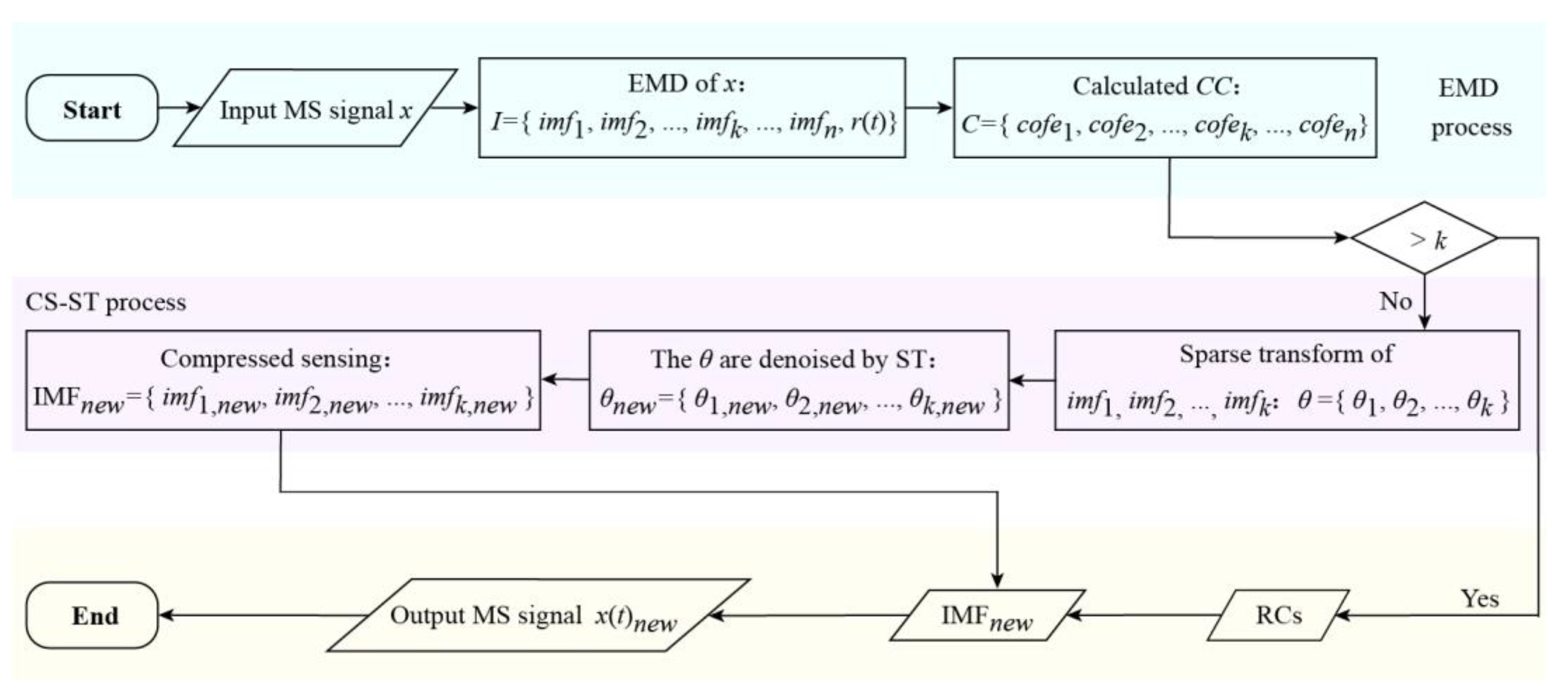
2. EMD_CS_ST Denoising Method

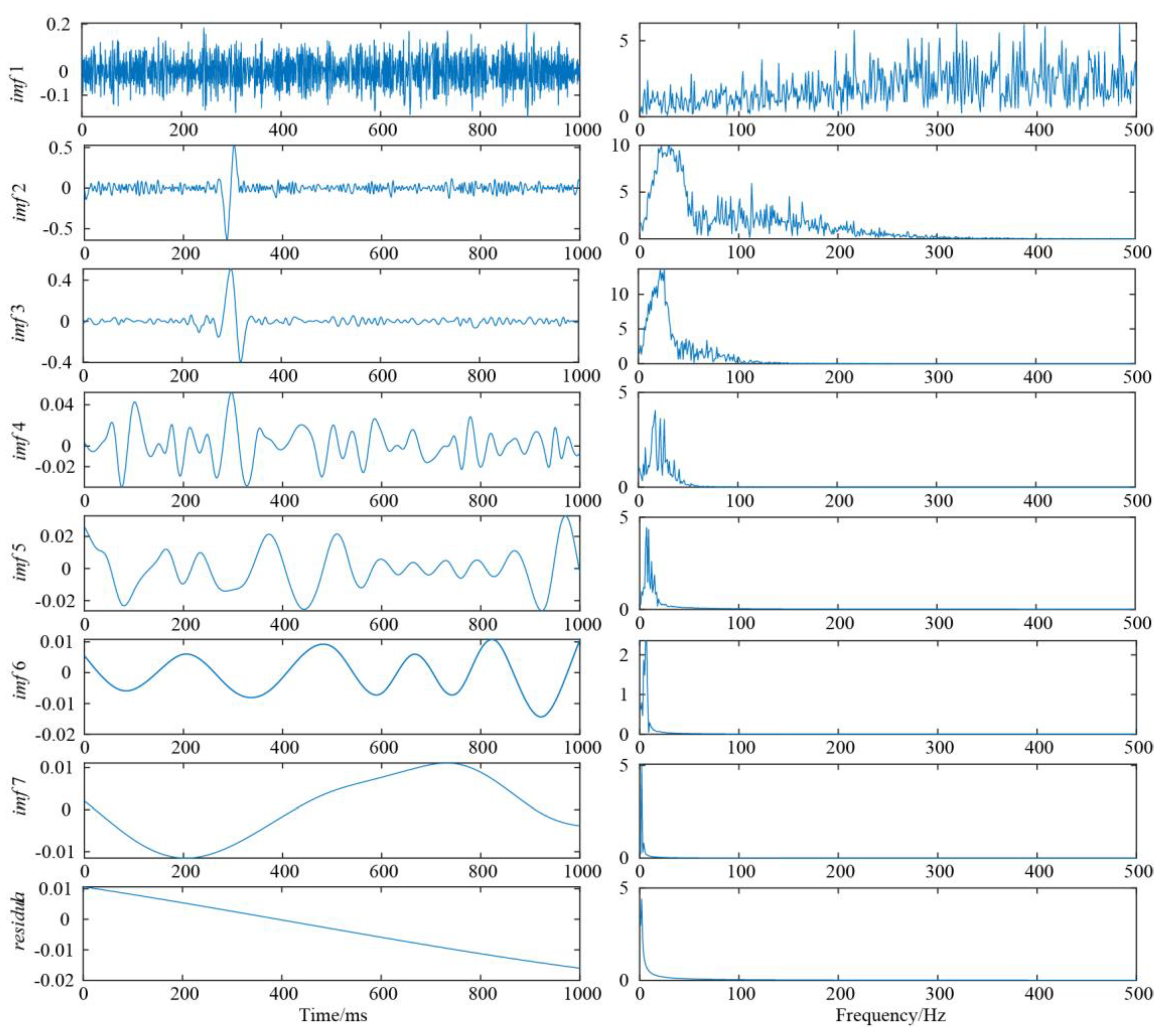
2.1. Empirical Mode Decomposition

The EMD method assumes that any complex signal consists of some simple Intrinsic Mode Functions (IMF) and that each IMF is independent of each other [26].

The IMF component must meet the following two conditions: (1) the number of extreme values and the number of zero crossings are the same or differ by at most one; (2) the upper and lower envelopes have local symmetry about the time axis. Any signal x(t) can be decomposed and can be expressed as follows:

$$x(t)={\displaystyle \sum _{i=1}^{n}i}m{f}_i(t)+r(t)$$

(1)

After decomposition, n IMF components are arranged in order of frequency from high to low, and the last one is the residual component r(t). Because the MS signal has the characteristics of low frequency and high energy, the noise in the MS signal is generally distributed in the higher frequency component, and the MS effective signal dominates the lower frequency component. Therefore, after the decomposition is completed, the components with more noise in the high-frequency region are discarded, and the residual components can be reconstructed to achieve denoising. The EMD method based on local features of signals has the advantages of a multi-resolution wavelet transform. It overcomes the difficulties in choosing a wavelet basis and determining the decomposition scale in the wavelet transform. It is suitable for signal analysis, non-linear and non-stationary. However, there may be some effective MS signals in the higher frequency components. If the high-frequency components are directly removed, signal distortion will inevitably occur [27,28].

According to the advantages of EMD decomposition, some scholars denoise the noise-containing components by determining the boundary component imf_k of the noise and the effective signal, and then reconstruct the residual components to obtain the denoised signal. The method of determining the boundary is as follows: Calculate the correlation coefficient Cofe between each IMF component and the original signal according to the following formula, denoted as C = {cofe₁, cofe₂, …, cofe_k, …, cofe_n}. Find the component that corresponds to the first minimum value in the coefficient C, and its next component is the boundary component between signal and noise, which is recorded as imf_k.

$$C(x,im{f}_i)=\frac{{\displaystyle \sum _{t=0}^{N-1}[x(t)-mean(x)][im{f}_i(t)-mean(im{f}_i)]}}{\sqrt{{\displaystyle \sum _{t=0}^{N-1}{[x(t)-mean(x)]}^2}}\sqrt{{\displaystyle \sum _{t=0}^{N-1}{[im{f}_i(t)-mean(im{f}_i)]}^2}}}$$

(2)

where x(t) is the original signal, imf_i(t) is the i-th IMF component, N is the number of sampling points, and mean is the mean function.

2.2. Compressed Sensing

CS theory has been widely used in information theory, image optimization, and other fields. It has accurate reconstruction ability for compressible target signals and has low requirements on sampling frequency. The basic idea of compressed sensing is the following: If the sparsity of an unknown signal is K or is transformed into K sparse by a sparse basis, then based on K sparse, combined with non-linear transformation, the original signal can be accurately reconstructed [21].

Let the expression of the noisy MS signal be:

$$x=X+e$$

(3)

where x is a noisy MS signal, X is a valid signal, and e is random noise.

The basic ideas of CS are as follows:

In the first step, a set of orthogonal basis matrices Ψ(N × N) is found to thin the MS signal x and obtain the sparse vector X₀:

$$X_0=\Psi x$$

(4)

In the second step, select a group of measurement matrix bases Φ (M × N, K < M < N), which are not related to the orthogonal basis, to project MS signal in low dimension, from N-dimension signal to M-dimension signal. Measured value y:

$$y=\Phi x$$

(5)

Combining Equations (4) and (5) gives:

$$y=\Phi {\Psi }^{-1}{X}_0=\Phi \theta$$

(6)

where θ is the coefficient to be reconstructed.

In the third step, in the case where the measured value y and the matrix Φ are known, the MS signal x is recovered from the measured value y with a high probability by an optimization method.

In the sparse transform domain, the effective signal X has sufficient sparsity, and the noise e does not have sparsity, so the noise cannot be restored in the process of signal reconstruction. This is the denoising principle of compressed sensing [22].

If the matrix Φ meets the Restricted Isometry Property (RIP) criterion, K sparse can obtain an optimal solution from the M measured values y. Since the dimension N of the coefficient to be reconstructed θ is much larger than the dimension M of the measured value y, the Equation (6) is an underdetermined system of formulas with an infinite set of solutions. Taking advantage of the sparsity of theta and using L1 norm regularization formula to find the optimal solution, it is a typical optimization algorithm to solve the underdetermined formula [29]:

$$\widehat{\theta }=\mathrm{argmin}\left\{\Vert y-\Phi \theta {\Vert }_2^2+\alpha \Vert \theta {\Vert }_1\right\}$$

(7)

Equation (7) is the theoretical basis of the compressed sensing algorithm, where || ||_p denotes the L_p norm; the first term in the braces is the constraint measurement term; the second term is the sparse constraint term, and the parameter α is the balance parameter. This paper chooses a sparse Bayesian learning algorithm that is more suitable for solving Equation (7) than the traditional L₁ norm regularization algorithm [30].

At present, commonly used measurement matrices include Gaussian random measurement matrices, random Bernoulli matrices, partially orthogonal matrices, Topliz and cyclic matrices and sparse random matrices, and other matrices. The Gaussian random measurement matrix is used as a universal compressed sensing matrix [31]. For this reason, it is used as the measurement matrix in this paper. The core idea is to construct the M × N measurement matrix Φ and make each element in the measurement matrix Φ obey the N(0,1/M) Gaussian distribution and conform to the RIP criterion. There is no correlation with most orthogonal bases [32]. The classical sparse transform methods include discrete cosine transform [33], discrete Fourier transform [34], discrete wavelet transform [35], and other transforms. In this paper, to organically combine with the following soft-thresholding denoising methods, a discrete wavelet transform is selected.

2.3. Soft-Thresholding

Wavelet threshold denoising is to distribute the energy of MS signals mainly in larger wavelet coefficients, and noise primarily distributed in smaller wavelet coefficients. Based on this distribution characteristic, the denoising can be achieved by converting the time domain signal into the wavelet domain and filtering the noise by setting an appropriate threshold value [36].

The key of the wavelet threshold is to select the appropriate threshold T to perform threshold quantization on the wavelet coefficients w_i,j of the noisy signal, to be as close as possible to the wavelet coefficient w of the original signal. Processed wavelet coefficients are represented as w₀, and wavelet reconstruction is performed to obtain a denoising signal.

Currently widely used is the data-driven threshold proposed by Donoho [36], the expression is as follows:

$$T_i=\frac{median\left\{\left|Y_i\right|\right\}}{0.6745}\sqrt{2\log N},(i=1,2,\cdots ,k)$$

(8)

where Y_i is the i-th IMF component, median is the median function, and T_i is the threshold of the i-th reconstruction coefficient θ_i.

Threshold denoising has a hard threshold and a soft thresholding. The hard thresholding function is better than the soft thresholding function in the sense of mean square error, but the signal will produce additional shocks, generate jumping points, and do not have the smoothness of the original signal, which greatly affects the initial pick-up of P wave and S wave of MS signal and the location of MS source. The overall continuity of the wavelet coefficients obtained from the soft threshold estimation is excellent, so that the estimated signal will not generate additional shocks, which is conducive to the later research work. Therefore, soft-thresholding denoising is used in this paper. The expression is:

$${\theta }_{i,new}=\{\begin{array}{ll}\mathrm{sgn}\left({\theta }_i\right)\cdot \left(\left|{\theta }_i\right|-T\right)\hfill & \left|{\theta }_i\right|⩾T\hfill \\ 0\hfill & \left|{\theta }_i\right|<T\hfill \end{array},(i=1,2,\cdots ,k)$$

(9)

where sgn is a symbol-function, and θ_i,new is a reconstruction coefficient after filtering the i-th IMF component.

2.4. EMD_CS_ST Denoising

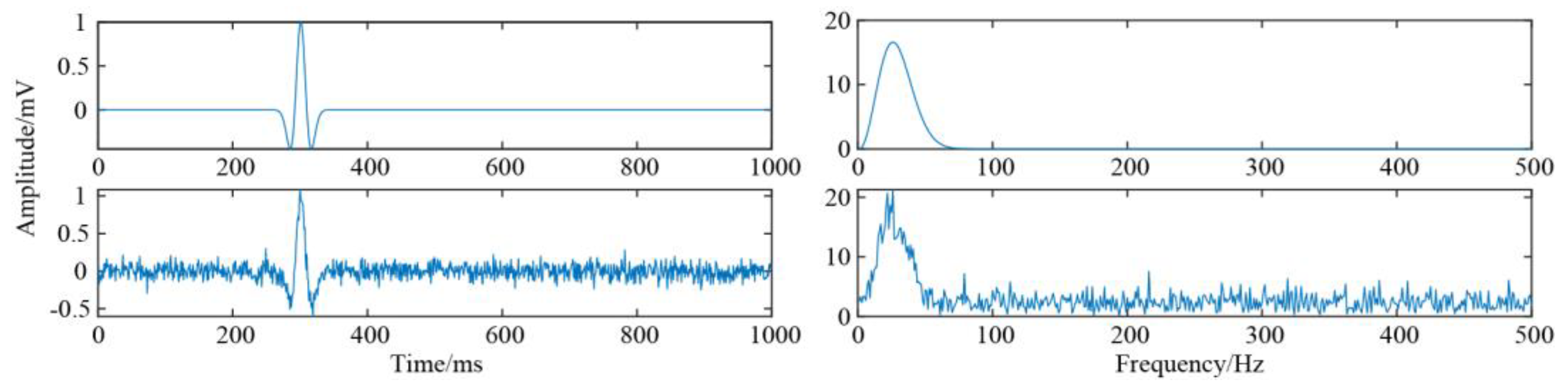
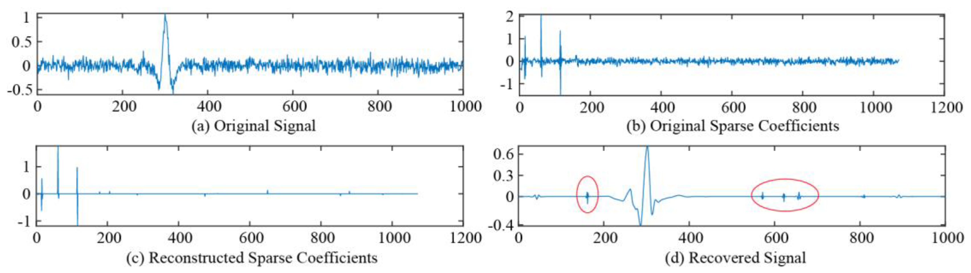
2.4.1. The Shortcomings of CS Denoising

To illustrate the problem of poor denoising performance when CS is facing a signal with a low signal-to-noise ratio. This paper verifies by digital simulation experiments. The Picker wavelet of the simulated seismic signal is used in the simulation experiment. The Picker wavelet can be expressed as:

$$f(t)=(1-2{\pi }^2{f}_p^2{t}^2)\exp (-{\pi }^2{f}_p^2{t}^2)$$

(10)

where f(t) is the amplitude, and f_p is the peak frequency. In the simulation analysis, f_p = 30 Hz, the sampling number is 1000, the sampling frequency is 1000 Hz, and random noise is added. The noise belongs to Gaussian distribution, and the variance is 0.09. Their waveforms and spectrums are shown in Figure 1.

Compressed sensing reconstruction of the noisy Ricker wavelet is shown in Figure 2. It can be known from Figure 2b that the original signal does not have sufficient sparsity in the sparse domain. After passing the CS algorithm, it can be seen from Figure 2c,d that the noise is removed, but the effect is not obvious, and the NF phenomenon (red circle) appears.

If soft-thresholding filtering is performed on the reconstruction coefficient θ and the sparse coefficient corresponding to the noise is removed, the obtained result is as shown in Figure 3. Although significant denoising was achieved, some NF phenomena (red circles) still appeared.

2.4.2. Improvement of CS Denoising

In view of the problems in Section 2.4.1, the MS signal is decomposed by EMD, and combined with the advantage of CS theory with certain denoising and soft-thresholding denoising, a method of denoising based on EMD_CS_ST is proposed. The specific steps of the denoising method are shown below.

Step 1: The EMD method is used to decompose the MS signal x(t) into a series of high-to-low frequency components, containing n IMF components and a residual component, denoted as I = {imf₁, imf₂, …, imf_k, …, imf_n, r(t)};

Step 2: Calculated the correlation coefficient of n IMF components by Equation (2), denoted as C = {cofe₁, cofe₂, …, cofe_k, …, cofe_n}, and found the first local minimum value of C, and the next IMF component corresponding to it is the boundary between noise and signal, recorded as imf_k;

Step 3: Performed discrete wavelet transform sparse processing on the imf_k component and the components before it, and calculated the coefficient θ to be reconstructed of k components, which are denoted as θ = {θ₁, θ₂, …, θ_k};

Step 4: Performed soft-thresholding filtering on the θ to obtain k reconstruction coefficients θ_new, which are denoted by θ_new = {θ_1,new, θ_2,new, …, θ_k,new };

Step 5: Reconstructed the reconstruction coefficient θ_new by CS to obtain k IMF_new, denoted as IMF_new = {imf_1,new, imf_2,new, …, imf_k,new };

Step 6: Recombined the k IMF_new components with the Remaining Components (RCs) to obtain the denoised signal, which is the effective MS signal x(t)_new after denoising.

The EMD_CS_ST algorithm flow chart is shown in Figure 4.

3. Simulation Experiment

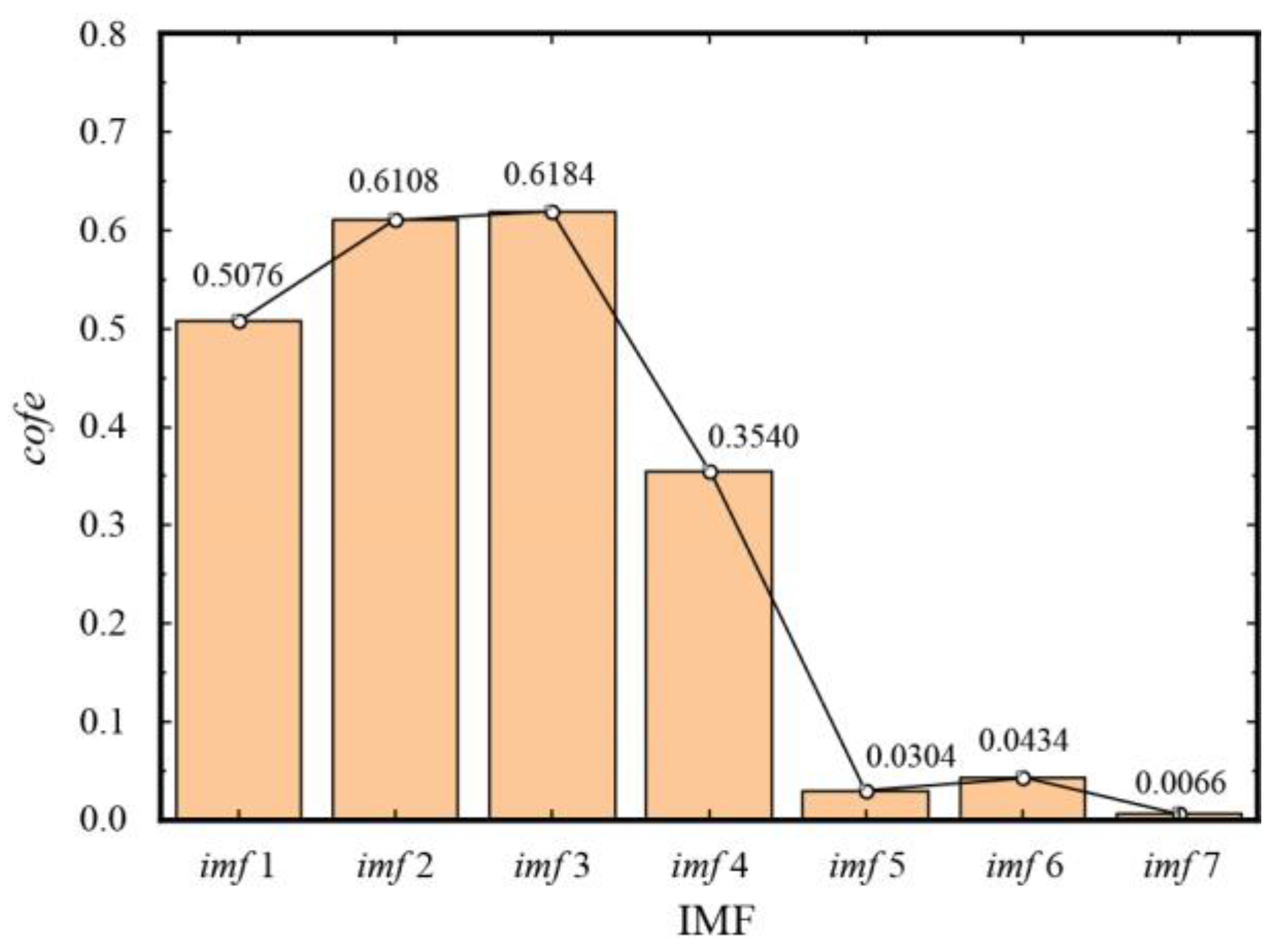
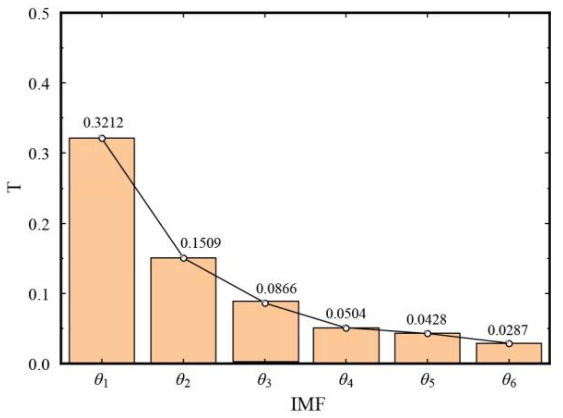
3.1. EMD_CS_ST Algorithm Application

Using the digital simulation analysis in Section 2.4.1, the EMD adaptive decomposition of the noisy Ricker wavelet is performed to obtain 7 IMF components. The waveforms of each component and its spectrum are shown in Figure 5.

The calculated cross-correlation coefficient is shown in Figure 6 with bar and dot charts. According to the demarcation point discrimination method of noise and signal, it can be known that imf₆ is a boundary. Then, the first six IMF components are respectively subjected to sparse transformation to obtain coefficients to be reconstructed θ = {θ₁, θ₂, …, θ₆}.

The threshold T is calculated according to the algorithm of Section 2.3, and the calculation result is shown in Figure 7, and soft-thresholding filtering is performed on the reconstruction coefficient θ. Finally, the denoised IMF_new component is reconstructed by discrete wavelet inverse transform, and the remaining IMF component is combined with IMF_new to obtain the denoised MS signal.

To further verify the effectiveness and feasibility of the proposed method, this paper compares with traditional discrete wavelet transform (DWT) denoising, EEMD denoising, and VMD_DWT [37] denoising methods. The simulation experiments of these denoising methods are carried out on the MATLAB platform. For the DWT denoising method of MS signals, the perform function is wdenoise, sym is used as the wavelet base, the number of filters is 8, and the number of decomposition layers is 5. The threshold rule is soft-threshold; estimate noise using only finest-scale wavelet coefficients. According to the signal-to-noise ratio (SNR), the signal standard deviation (SD), the correlation coefficient (CC) of the pure signal, and the denoising signal, these three indicators quantitatively illustrate the denoising effect of this paper. The waveforms and their spectra after denoising by these four methods are shown in Figure 8.

The SNR is defined as:

$$SNR=10\log \left\{\frac{{\displaystyle \sum _{t=0}^{N-1}x}{(t)}^2}{{\displaystyle \sum _{t=0}^{N-1}{\left[x(t)-x{(t)}_{new}\right]}^2}}\right\}$$

(11)

where x(t) is a pure signal, x(t)_new is a denoised signal, and N is the number of sampling points. If the signal has a high SNR after denoising, the denoising effect is better.

The SD is defined as:

$$SD=\sqrt{{\displaystyle \sum _{t=0}^{N-1}{\left[x(t)-x{(t)}_{new}\right]}^2}/N}$$

(12)

If the SD is smaller, it means that the smaller the fluctuation between the denoising signal and the pure signal, the closer to the pure signal.

The CC between the pure signal and the denoising signal is defined as:

$$CC=\frac{\mathrm{Cov}\left[x(t),x{(t)}_{new}\right]}{\sqrt{\mathrm{Var}[x(t)]\cdot \mathrm{Var}\left[x{(t)}_{new}\right]}}$$

(13)

where Cov is the covariance function, Var is the variance function. If the CC value is closer to 1, the denoising signal is similar to the clean signal.

Apply the Equations (11)–(13) to calculate the SNR before and after denoising of the noisy Picker wavelet, and the SD and CC after denoising. These results are shown in

Table 1. Four methods for comparative analysis of the denoise effect.

Category	B-SNR	A-SNR	SD	CC
EMD_CS_ST	4.651	27.170	0.028	0.972
DWT	4.651	22.624	0.035	0.955
EEMD	4.651	21.285	0.038	0.945
VMD_DWT	4.651	23.680	0.034	0.952

.

It can be seen from Table 1 and Figure 8 that the EMD_CS_ST has a better denoising effect than the other three methods. Analysis from Table 1 shows that the SNR of the noisy Ricker wavelet is 4.651 dB. After applying this method, the SNR is increased to 27.170 dB, the signal standard deviation is the smallest, and the correlation coefficient is the largest. Transient non-stationary characteristics of the MS signal are fully preserved compared to the other three methods.

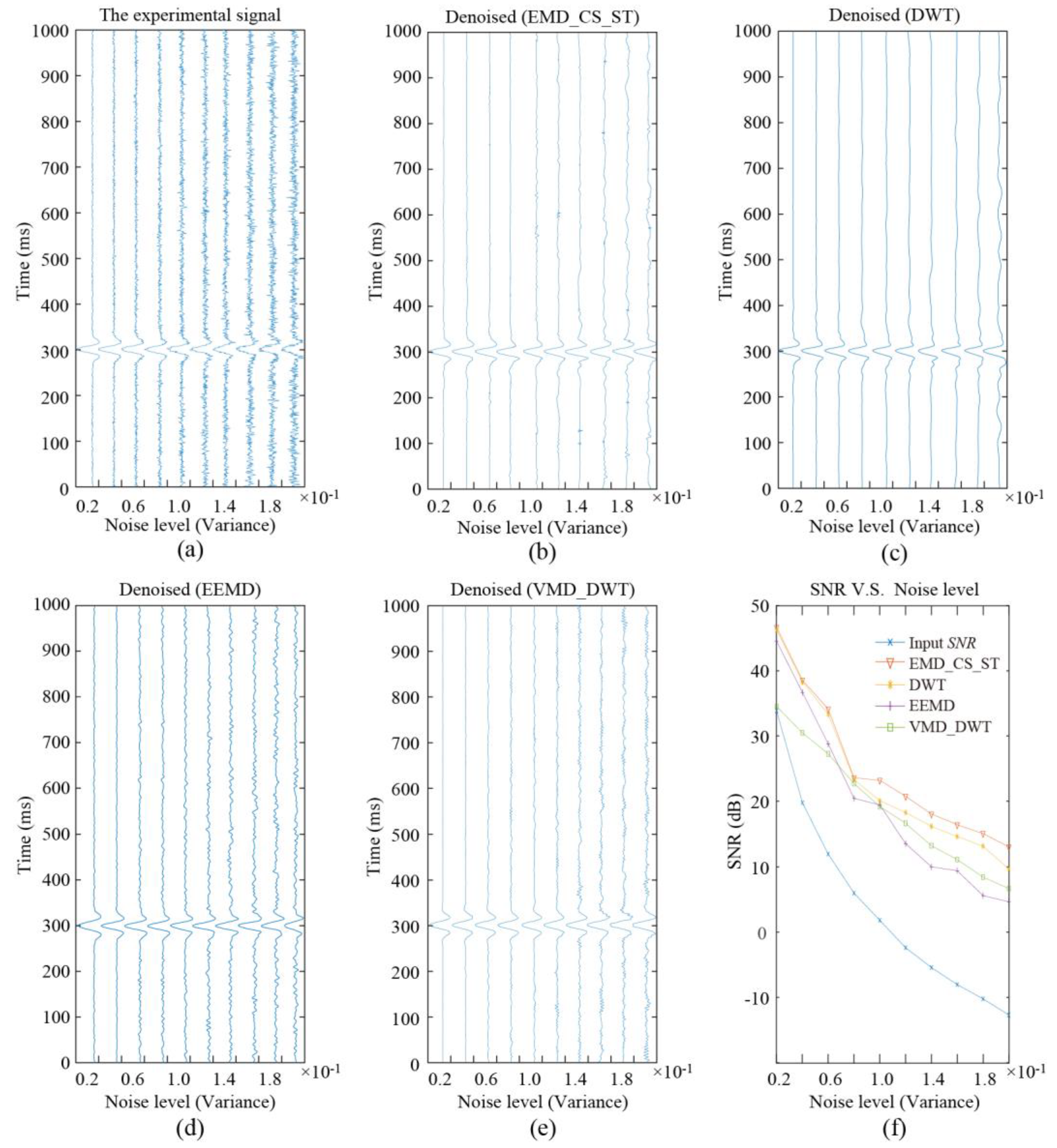
3.2. Comparison of Denoising Effects at Different Noise Levels

To test the performance of the four methods at different noise levels, we added 10 sets of random noise at different levels to the pure signal, and the noise variance changed from 0.02 to 0.20. Signals with different input noise levels, denoised signals, and SNR are shown in Figure 9. Figure 9f shows the SNR at different noise levels and the SNR after denoising. The red line is the proposed method. It can be seen directly from Figure 9f that the red line corresponding to this method is at the top of all other lines, indicating that the denoising effect is the best. When faced with high SNR signals, the proposed method is equivalent to DWT denoising, but when faced with low SNR signals, the proposed method seems to perform better than other methods. This phenomenon indicates that the proposed method is more effective for signals with higher noise levels.

4. Case Study

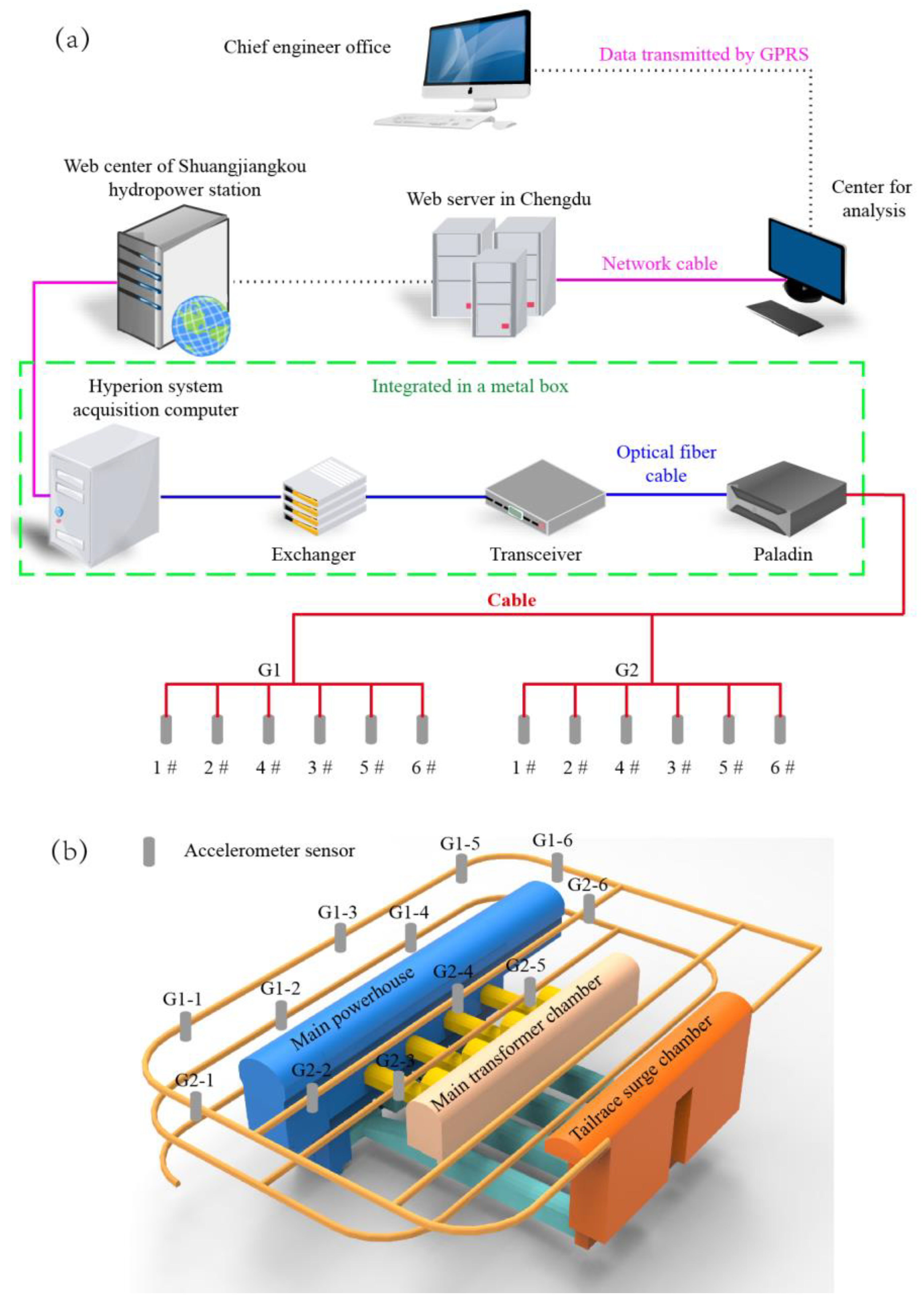
4.1. Description of the MS Monitoring System and Actual MS Signal

The actual MS signal comes from the safety construction monitoring system of the underground chamber of Shuangjiangkou Hydropower Station in Southwest China. In view of the severe problem of rock mass deformation and rockburst disasters in the underground main powerhouse, the seismic monitoring system of the Canadian Engineering Seismology Group (ESG) was adopted [38,39,40]. The seismic monitoring system mainly includes Paladin digital signal acquisition system, Hyperion digital signal processing system, acceleration sensor, cable fiber, and so on, as shown in Figure 10a. In the underground main powerhouse, two groups of acceleration sensors were installed; each group has six. They were installed in the upper and middle drainage gallery, as shown in Figure 10b. The monitoring region mainly covers the main powerhouse, involving the main transformer chamber, the surrounding rock of part of the pressure pipeline.

The acceleration sensors with a frequency response of 20 Hz to 5000 Hz were arranged in a spatial network distribution. The sensitivity of the acceleration sensor is 30 V/g, and the Paladin digital signal acquisition system has a sampling frequency of 10 kHz. According to the Short Time Average and Longtime Average algorithms (STA/LTA), the threshold of the trigger channel is set to 4. If multiple sensors detect the seismic waves generated by a rock fracture and the corresponding value exceeds the threshold, the sensors record them immediately. These recorded electrical signals will be sent to the digital acquisition system for processing and transmitted to WaveVis software via fiber optic cables to obtain a valid MS signal [41]. Often, the signal received by the system is not only the signal generated by rock fracture but also some blasting, mechanical vibration, current sound, and other noise signals. These mixed signals need to be denoised. After the acquisition, these electrical signals are transmitted to the processing system via fiber optic cables.

4.2. Field Data Examples

The ESG system has been operating in the main powerhouse of the Shuangjiangkou hydropower station for two years, during which thousands of MS events were obtained. Three groups of effective MS signals were randomly selected for EMD_CS_ST de-noising processing and analysis. To facilitate calculation and comparison, the effective MS signals are intercepted 1000 ms from each time-window of 1500 ms. Firstly, three groups of signals are denoised by the method of EMD_CS_ST, and then using the MATLAB platform to perform FFT spectrum analysis, it can more intuitively judge the denoising effect of MS signals. The waveform and time spectrum before and after denoising are shown in Figure 11.

It can be seen from Figure 11 that the three groups of original MS signals all contain a large amount of random noise. Even if the main spectrum distribution of these signals can be seen from the time spectrum, it is not obvious due to noise interference. After the denoising processing of this method, the waveform and time spectrum of the MS signal are clearer, the dominant spectrum is more visible, and there is almost no NF phenomenon. The EMD_CS_ST method was adopted to denoise MS signal, and the signal denoised has the advantages of high SNR and stable waveform. The effectiveness and practicability of the proposed method are proved qualitatively.

5. Conclusions

Considering that the MS signal contains a large amount of random noise, an EMD_CS_ST denoising method was proposed, and the advantages and disadvantages of the EMD_CS_ST, DWT, EEMD, and VMD_DWT are compared and analyzed through a numerical simulation experiment. The denoising analysis of MS signals obtained from the underground cavern of Shuangjiangkou hydropower station was carried out. The following conclusions are drawn.

The numerical simulation experiment demonstrates the NF phenomenon of the compressed sensing denoising method in the process of signal reconstruction with low SNR. Although the theory of CS has a certain ability to reduce noise in the denoising of MS signals, the effect is weak.

The CS denoising method is not suitable for direct application to the denoising processing of MS signals. The EMD_CS_ST method can better compensate for the deficiency of CS in MS signal denoising and greatly weaken the NF phenomenon caused by CS.

Simulation experiments were conducted to compare the effects of four kinds of MS signal denoising methods such as EMD_CS_ST, DWT, EEMD, and VMD_DWT. The FFT time spectrum of MS signals before and after denoising were compared and analyzed. The feasibility of the EMD_CS_ST method is demonstrated qualitatively.

By introducing the SNR, the SD, and the CC, the rationality and effectiveness of the EMD_CS_ST method were proved quantitatively. The actual three MS signals were denoised, and the effect was remarkable.

The CS technology itself has matured, and we can apply EMD_CS_ST to data collection, storage, and noise reduction in the later stage to achieve integrated data processing of the three, which can greatly reduce the space occupied by data.

References

1. Li, A.; Liu, Y.; Dai, F.; Liu, K.; Wei, M.D. Continuum analysis of the structurally controlled displacements for large-scale underground caverns in bedded rock masses. Tunn. Undergr. Sp. Technol. 2020, 97, 103288. [Google Scholar] [CrossRef]
2. Zhao, Y.; Yang, T.; Bohnhoff, M.; Zhang, P.; Yu, Q.; Zhou, J.; Liu, F. Study of the Rock Mass Failure Process and Mechanisms During the Transformation from Open-Pit to Underground Mining Based on Microseismic Monitoring. Rock Mech. Rock Eng. 2018, 51, 1473–1493. [Google Scholar] [CrossRef]
3. Xu, J.; Jiang, J.; Liu, Q.; Gao, Y. Stability Analysis and Failure Forecasting of Deep-Buried Underground Caverns Based on Microseismic Monitoring. Arab. J. Sci. Eng. 2018, 43, 1709–1719. [Google Scholar] [CrossRef]
4. Dai, F.; Li, B.; Xu, N.; Meng, G.; Wu, J.; Fan, Y. Microseismic Monitoring of the Left Bank Slope at the Baihetan Hydropower Station, China. Rock Mech. Rock Eng. 2017, 50, 225–232. [Google Scholar] [CrossRef]
5. Li, H.; Wang, R.; Cao, S.; Chen, Y.; Huang, W. A method for low-frequency noise suppression based on mathematical morphology in microseismic monitoring. Geophysics 2016, 81, V159–V167. [Google Scholar] [CrossRef]
6. Iqbal, N.; Zerguine, A.; Kaka, S.; Al-Shuhail, A. Observation-driven method based on IIR Wiener filter for microseismic data denoising. Pure Appl. Geophys. 2018, 175, 2057–2075. [Google Scholar] [CrossRef]
7. To, A.C.; Moore, J.R.; Glaser, S.D. Wavelet denoising techniques with applications to experimental geophysical data. Signal Process. 2009, 89, 144–160. [Google Scholar] [CrossRef]
8. Li, J.; Li, Y.; Li, Y.; Qian, Z. Downhole microseismic signal denoising via empirical wavelet transform and adaptive thresholding. J. Geophys. Eng. 2018, 15, 2469–2480. [Google Scholar] [CrossRef] [Green Version]
9. Han, J.; Mirko, V.D.B. Microseismic and seismic denoising via ensemble empirical mode decomposition and adaptive thresholding. Geophysics 2015, 80, KS69–KS80. [Google Scholar] [CrossRef] [Green Version]
10. Liang, Z.; Peng, S.; Zheng, J. Self-adaptive denoising for microseismic signal based on EMD and mutual information entropy. Comput. Eng. Applicat. 2014, 50, 7–11. [Google Scholar] [CrossRef]
11. Zuo, L.Q.; Sun, H.M.; Mao, Q.C.; Liu, X.Y.; Jia, R.S. Noise Suppression Method of Microseismic Signal Based on Complementary Ensemble Empirical Mode Decomposition and Wavelet Packet Threshold. IEEE Access 2019, 7, 176504–176513. [Google Scholar] [CrossRef]
12. Haghighatshoar, S.; Abbe, E. Polarization of the Rényi Information Dimension with applications to compressed sensing. IEEE Trans. Inform. Theory 2017, 63, 6858–6868. [Google Scholar] [CrossRef] [Green Version]
13. Deng, Q.; Zeng, H.; Zhang, J.; Tian, S.; Cao, J.; Li, Z.; Liu, A. Compressed sensing for image reconstruction via back-off and rectification of greedy algorithm. Signal Process. 2019, 157, 280–287. [Google Scholar] [CrossRef]
14. Mammone, N.; De Salvo, S.; Ieracitano, C.; Marino, S.; Cartella, E.; Bramanti, A.; Giorgianni, R.; Morabito, F.C. Compressibility of High-Density EEG Signals in Stroke Patients. Sensors 2018, 18, 4107. [Google Scholar] [CrossRef] [PubMed] [Green Version]
15. Mammone, N.; De Salvo, S.; Bonanno, L.; Ieracitano, C.; Marino, S.; Marra, A.; Morabito, F.C. Brain network analysis of compressive sensed high-density EEG signals in AD and MCI subjects. IEEE Trans. Ind. Inform. 2018, 15, 527–536. [Google Scholar] [CrossRef]
16. Bevacqua, M.T.; Crocco, L.; Di Donato, L.; Isernia, T. Non-linear inverse scattering via sparsity regularized contrast source inversion. IEEE Trans. Comput. Imag. 2017, 3, 296–304. [Google Scholar] [CrossRef]
17. Bevacqua, M.T.; Isernia, T. Boundary indicator for aspect limited sensing of hidden dielectric objects. IEEE Geosci. Remote Sens. 2018, 15, 838–842. [Google Scholar] [CrossRef]
18. Nianmin, G.; Meng, C.; Xuemei, F.; Haijun, S.; Ruirui, Z. Seismic data reconstruction method based compressed sensing theory. In Proceedings of the SPG/SEG 2016 International Geophysical Conference, Beijing, China, 20–22 April 2016; Society of Exploration Geophysicists and Society of Petroleum Geophysicists: Beijing, China, 2016; pp. 713–715. [Google Scholar] [CrossRef]
19. Sun, Y.Y.; Jia, R.S.; Sun, H.M.; Zhang, X.L.; Peng, Y.J.; Lu, X.M. Reconstruction of seismic data with missing traces based on optimized Poisson Disk sampling and compressed sensing. Comput. Geosci. 2018, 117, 32–40. [Google Scholar] [CrossRef]
20. Sun, M.; Li, Z.; Li, Z.; Li, Q.; Li, C.; Zhang, H. Reconstruction of seismic data with weighted MCA based on compressed sensing. Chin. J. Geophys. Chin. 2019, 62, 1007–1021. (In Chinese) [Google Scholar] [CrossRef]
21. Donoho, D.L. Compressed sensing. IEEE Trans. Inform. Theory. 2006, 52, 1289–1306. [Google Scholar] [CrossRef]
22. Zhu, L.; Zhu, Y.; Mao, H.; Gu, M. A new method for sparse signal denoising based on compressed sensing. In Proceedings of the 2009 2nd International Symposium on Knowledge Acquisition and Modeling, KAM 2009, Wuhan, China, 30 November–1 December 2009; IEEE Computer Society: Wuhan, China, 2009; pp. 35–38. [Google Scholar] [CrossRef]
23. Arias-Castro, E.; Eldar, Y.C. Noise folding in compressed sensing. IEEE Signal Proc. Lett. 2011, 18, 478–481. [Google Scholar] [CrossRef] [Green Version]
24. Davenport, M.A.; Laska, J.N.; Treichler, J.R.; Baraniuk, R.G. The pros and cons of compressive sensing for wideband signal acquisition: Noise folding versus dynamic range. IEEE Trans. Signal Procs. 2012, 60, 4628–4642. [Google Scholar] [CrossRef]
25. Wen, F.; Zhang, G.; Tao, Y.; Liu, S.; Feng, J. Adaptive compressive sensing toward low signal-to-noise ratio scene. Acta Phys. Sin. Chin. Ed. 2015, 64, 84301. (In Chinese) [Google Scholar] [CrossRef]
26. Huang, N.E.; Shen, Z.; Long, S.R.; Wu, M.C.; Shih, H.H.; Zheng, Q.; Yen, N.C.; Tung, C.C.; Liu, H.H. The empirical mode decomposition and the Hilbert spectrum for nonlinear and non-stationary time series analysis. Proc. R. Soc. 1998, 903–995. [Google Scholar] [CrossRef]
27. Li, Y.; Peng, J.; Ma, H.; Lin, H. Study of the influence of transition IMF on EMD do-noising and the improved algorithm. Chin. J. Geophys. Chin. 2013, 56, 626–634. (In Chinese) [Google Scholar] [CrossRef]
28. Wu, Z.; Huang, N.E. Ensemble empirical mode decomposition: A noise-assisted data analysis method. Advan. Adapt. Data Anal. 2009, 1, 1–41. [Google Scholar] [CrossRef]
29. Candes, E.J.; Wakin, M.B.; Boyd, S.P. Enhancing Sparsity by Reweighted ℓ 1 inimization. J. Fourier Ananl. Appl. 2008, 14, 877–905. [Google Scholar] [CrossRef]
30. Tipping, M.E. Sparse Bayesian Learning and the Relevance Vector Machine. J. Mach. Learn. Res. 2001, 1, 211–244. [Google Scholar] [CrossRef] [Green Version]
31. Candes, E.J.; Tao, T. Decoding by linear programming. IEEE Trans. Inform. Theory 2005, 51, 4203–4215. [Google Scholar] [CrossRef] [Green Version]
32. Baraniuk, R. Compressive sensing [Lecture notes]. IEEE Signal Proc. Mag. 2007, 24, 118–121. [Google Scholar] [CrossRef]
33. Ahmed, N.; Natarajan, T.; Rao, K. Discrete Cosine Transform. IEEE Trans. Comput. 1974, 23, 90–93. [Google Scholar] [CrossRef]
34. Bluestein, L.I. A linear filtering approach to the computation of discrete Fourier transform. IEEE Trans. Audio Electroacoust. 1970, 18, 451–455. [Google Scholar] [CrossRef] [Green Version]
35. Chang, C.; Girod, B. Direction-adaptive discrete wavelet transform for image compression. IEEE Trans. Image Process. 2007, 16, 1289–1302. [Google Scholar] [CrossRef] [PubMed] [Green Version]
36. Donoho, D.L. De-noising by soft-thresholding. IEEE Trans. Inform. Theory 1995, 41, 613–627. [Google Scholar] [CrossRef] [Green Version]
37. Zhang, W.; Zhang, M.; Zhao, Y.; Jin, B.; Dai, W. Denoising of the Fiber Bragg Grating Deformation Spectrum Signal Using Variational Mode Decomposition Combined with Wavelet Thresholding. Appl. Sci. 2019, 9, 180. [Google Scholar] [CrossRef] [Green Version]
38. Dai, F.; Li, B.; Xu, N.; Zhu, Y. Microseismic early warning of surrounding rock mass deformation in the underground powerhouse of the Houziyan hydropower station, China. Tunn. Undergr. Sp. Technol. 2017, 62, 64–74. [Google Scholar] [CrossRef]
39. Xu, N.; Li, T.; Dai, F.; Li, B.; Zhu, Y.; Yang, D. Microseismic monitoring and stability evaluation for the large scale underground caverns at the Houziyan hydropower station in Southwest China. Eng. Geol. 2015, 188, 48–67. [Google Scholar] [CrossRef]
40. Xu, N.; Dai, F.; Li, B.; Zhu, Y.; Zhao, T.; Yang, D. Comprehensive evaluation of excavation-damaged zones in the deep underground caverns of the Houziyan hydropower station, Southwest China. Bull. Eng. Geol. Env. 2017, 76, 275–293. [Google Scholar] [CrossRef]
41. Xiao, H.; Xu, Z.; Lyu, S. Quasi-Steady-State scheme and application on prewhirl flow and heat transfer in aeroengine. Int. J. Precis. Eng. Man 2015, 16, 343–350. [Google Scholar] [CrossRef]
Figure 1. Ricker waveform, noisy Ricker waveform, and their spectrums.
Applsci 10 02191 g001
Figure 2. Ricker waveform reconstructed by compressed sensing. (a) Original signal, (b) original sparse coefficients, (c) reconstructed sparse coefficients, and (d) recovered signal.
Applsci 10 02191 g002
Figure 3. Ricker waveform after compressed sensing threshold denoising. (a) The original signal, (b) original sparse coefficients, (c) reconstructed sparse coefficients, and (d) recovered signal.
Applsci 10 02191 g003
Figure 4. The EMD_CS_ST algorithm flow chart. First, Empirical Mode Decomposition (EMD) is performed on the MS signal. Then, CS_ST is used to denoise the Intrinsic Mode Functions (IMF) components to be denoised. Finally, the denoised components and the remaining IMF components are combined to obtain the final effective signal.
Applsci 10 02191 g004
Figure 5. EMD decomposed the results of the noise Ricker waveform and the IMF’s corresponding spectrum.
Applsci 10 02191 g005
Figure 6. Correlation coefficients of signal and IMF.
Applsci 10 02191 g006
Figure 7. The T value of the coefficient to be reconstructed of the first 6 components IMF.
Applsci 10 02191 g007
Figure 8. Four methods for denoised of the Ricker waveform and their spectra.
Applsci 10 02191 g008
Figure 9. The comparative experiments under different noise levels. (a) The original signal. (b) The EMD_CS_ST denoised signal. (c) The DWT denoised signal. (d) The EEMD denoised signal. (e) The VMD_DWT denoised signal. (f) The SNR before and after denoising.
Applsci 10 02191 g009
Figure 10. The layout of the MS monitoring system in the main powerhouse. (a) The MS monitoring system network topology. (b) The layout of the acceleration sensor.
Applsci 10 02191 g010
Figure 11. The waveform before and after denoising of the MS signal, and their time-frequency spectrum.
Applsci 10 02191 g011