Article

Parallelization of the Honeybee Search Algorithm for Object Tracking

by
Oscar E. Perez-Cham
1,
Cesar Puente
1,
Carlos Soubervielle-Montalvo
1,*,
Gustavo Olague
2,
Carlos A. Aguirre-Salado
1 and
Alberto S. Nuñez-Varela
1
1
Faculty of Engineering, Autonomous University of San Luis Potosi, Dr. Manuel Nava 8, Zona Universitaria Poniente, San Luis Potosi 78290, SLP, Mexico
2
EvoVisión Laboratory, CICESE Research Center, Carretera Ensenada-Tijuana 3918, Playitas, Ensenada 22860, BC, Mexico
*
Author to whom correspondence should be addressed.
Appl. Sci. 2020, 10(6), 2122; https://doi.org/10.3390/app10062122
Submission received: 27 December 2019 / Revised: 7 March 2020 / Accepted: 13 March 2020 / Published: 20 March 2020
(This article belongs to the Section Computing and Artificial Intelligence)

Abstract

:
Object tracking refers to the relocation of specific objects in consecutive frames of a video sequence. Presently, this visual task is still considered an open research issue, and the computer science community attempted solutions from the standpoint of methodologies, algorithms, criteria, benchmarks, and so on. This article introduces a GPU-parallelized swarm algorithm, called the Honeybee Search Algorithm (HSA), which is a hybrid algorithm combining swarm intelligence and evolutionary algorithm principles, and was previously designed for three-dimensional reconstruction. This heuristic inspired by the search for food of honeybees, and here adapted to the problem of object tracking using GPU parallel computing, is extended from the original proposal of HSA towards video processing. In this work, the normalized cross-correlation (NCC) criteria is used as the fitness function. Experiments using 314 video sequences of the ALOV benchmark provides evidence about the quality regarding tracking accuracy and processing time. Also, according to these experiments, the proposed methodology is robust to high levels of Gaussian noise added to the image frames, and this confirms that the accuracy of the original NCC is preserved with the advantage of acceleration, offering the possibility of accelerating latest trackers using this methodology.

1. Introduction

Object tracking deals with the problem of following a specific object from a video source in a frame by frame basis, and tries to solve several challenges such as the occlusion of objects [1,2]; and the abrupt changes in light, color or size [3]. Different approaches, known as trackers, have been proposed in order to solve the object tracking problem, but no definitive answer has been found [3,4,5,6,7]. Usually, researchers compare trackers against each other regarding speed and accuracy with focus on trackers which provide the most accurate results but have considerable low speeds.
In general, trackers are slower because they perform more operations to provide better accuracy. This apparent negative correlation between accuracy and speed makes it challenging to select a suitable tracker for any given application [8]. In summary, the studied problem in this work is how to accelerate a specific tracker without having negative effects on their accuracy.
The Graphics Processing Unit (GPU) is a useful tool to accelerate computational tasks in general, including object tracking [9,10]. This device thrives at the moment of accelerating trackers such as the Normalized Cross-Correlation (NCC) [11,12,13]. Although NCC is not a recent tracker it is one of the most studied trackers due to its low complexity and good performance regarding accuracy. NCC is well positioned compared to other trackers that used the ALOV video dataset for testing and evaluation [3]. Moreover, this work presents a GPU-based parallel version of the Honeybee Search Algorithm (HSA, detailed in Section 2.2) [14,15,16,17] to achieve greater NCC acceleration. While a GPU allows accelerating computations by performing numerous operations in parallel, HSA achieves acceleration by performing a heuristic search rather than an exhaustive search. In other words, HSA, such as other heuristics, converges to the optimal solutions after several iterations. It is important to mention that HSA is considered a pioneer on the subject of bio-inspired bees applied to the field of artificial intelligence [18].
Adaptation of Swarm Intelligence (SI) algorithms, such as HSA, for parallel execution on a GPU, is not a new idea. The research of Tan and Ding [19] proposes that when an SI algorithm is parallelized through the GPU, the implementation must fall in one of the following four categories: (1) naïve parallel model, (2) multiphase parallel model, (3) all-GPU parallel model, or (4) multiswarm parallel model. They identified those models by observing several parallel implementations of SI algorithms [20,21,22,23,24], most of which are based on the Particle Swarm Optimization heuristic. We selected HSA for this study as it differs from other SI algorithms on the following basis: (1) it can be used for real-valued optimization problems, while other heuristics are limited to discrete problems, (2) it is not explicitly designed for route searching problems, and (3) according to our knowledge, the parallelization of HSA has not been proposed or developed for object tracking.
SI has been used for object tracking in a few works [25,26], but as far as we know, the parallelized SI algorithms have been mostly tested with benchmarking functions, and less frequently used for object tracking [27]. This work uses the unique combination of: NCC as the tracker function, the HSA for heuristic search, and a GPU for hardware acceleration.
Experiments performed within this work show that the addition of HSA improves the speed against a purely GPU-accelerated NCC. Also, there are no observed adverse effects on the accuracy of the results and these are confirmed using a proposed evaluation criterion, called Score-Time Efficiency. The Score-Time Efficiency is used to facilitate the comparison of different tracker proposals regarding speed and accuracy. This work can be considered a proof of concept to increase the acceleration of object tracking by parallelizing HSA using the GPU with the NCC tracker as its fitness function.
This work is organized as follows: Section 2 describes the materials and methods, starting with a description of the honeybee dance language (Section 2.1) that serves as an inspiration for HSA (Section 2.2). Later, the Normalized Cross-Correlation (Section 2.3) tracker is described in detail, allowing us to understand its application as a fitness function (Section 2.4) for HSA and parallelized using a GPU (Section 2.5). We detail the procedure used to test the accuracy and speed of the different implementations in Section 2.6. Additionally, Section 3 presents the results of the different conducted experiments. Section 4 gives the discussion of the results. Finally, Section 5 provides the conclusion and future work.

2. Materials And Methods

2.1. The Honeybee Dance Language

The information shared by honeybees through their dance language [28] is the location, quality, and quantity of food they have found. Honeybees may take a long time to find food, depending on how far it is from their hive. Nevertheless, once one of them locates the source of food, then other honeybees swarm around it, making it clear that they have been taught where to go. The honeybee dance is never displayed if there are no other honeybees, which is proof that it is a communications tool that requires an audience.
While these insects are recruiting, they use odor samples to identify the location of resources, as well as the desirability of a resource. The possible recruits can confirm the quality of the food source by smelling samples brought by the explorer. The quantity of food is related to the “liveliness” and “enthusiasm” of the dance performance. The dancer makes pauses for antennal contact with peers, to transfer some harvested samples of nectar. The angle recorded by bees during their trajectory to the resource, relative to the sun’s azimuth (the horizontal component of direction towards the sun), is mirrored following the angle on the comb using the waggle portion of the dance.
The described process can be abstracted and represented using pseudocode, which can be useful to develop an algorithm. Algorithm 1 shows a very general view of the search process employed by honeybees. There are three main phases: exploration, recruitment, and harvest. The process is inherently parallel and the algorithm could be improved by embracing parallel processing technologies.
Algorithm 1 HSA is divided into 3 phases: exploration, recruitment, and harvest.
  Honeybee Search Algorithm()
 1 Exploration()
 2 Recruitment()
 3 Harvest()

2.2. The Honeybee Search Algorithm

The following section provides more details of HSA used as the basis for this work. The algorithm was initially proposed by Olague and Puente [14,15,16] defined as a meta-heuristic that combines Evolutionary Algorithms and Swarm Intelligence with individuals that emulate the behavior of foraging honeybees. As displayed in Algorithm 1, there are three main phases: exploration, recruitment, and harvest. The exploration phase consists of sending search agents called explorers to random points of a specific multidimensional space; these points or possible solutions are called food sources. We define the richness or attractiveness of the food sources through a function called fitness function. The next phase, recruitment, is where the explorers return to the hive and try to convince other honeybees to follow them to exploit the food source they have found. In the last phase, harvest, a massive search covers the space where the surroundings of the best food sources receive considerable greater attention. An evolutionary algorithm similar to Evolution Strategies ( μ + λ ) is at the core of in the harvest and exploration phases; mutation and crossover are used as the leading evolutionary operators [29].
The exploration stage (Algorithm 2) is actually a modified Evolution Strategy (ES) of the type μ + λ . These evolutionary algorithms serve as a simulation of the natural process in which the honeybees perform asynchronous exploration of the space in search of the food source. The exploration stage starts creating a random population μ e of multidimensional points called explorers, which are then transformed into a new population λ e using the mutation, crossover, and random steps. The best individuals are selected using a fitness value as criteria, obtained using a fitness function. The importance of mutation commonly distinguishes this kind of Evolutionary Algorithm as the main source of change between generations (instead of crossover). In this case, we follow the approach proposed by Boumaza and Louchet [30], with some changes in operators used to evolve the population. λ e sons are generated by three different methods: α e sons are generated by Polynomial Mutation [29], β e sons are generated by crossover using Simulated Binary Crossover [29] and γ e sons are generated randomly. It should be noted that α e + β e + γ e = λ e . Another important difference between the common ES and the one used in this algorithm is that a sharing operator [31] is used to penalize individuals that concentrate in a small space by reducing the individual’s fitness value. The algorithm repeats this stage until a given number of iterations or generations.
The recruiting phase is easily understood: we divide the total number λ of forager agents into groups. The proportional size p i of those groups is relative to the fitness value ( f i t i ) of each of the individuals that were selected from the exploration phase, as seen in Equation (1). Not all explorers may have assigned foragers to harvest their location; these might not have found a food source that is good enough.
p i = f i t i j = 1 μ e f i t j
r i = p i × μ h
The harvest phase (Algorithm 3) is also a ( μ + λ )-ES where the offspring is generated in the exact same way as in the exploration phase ( λ h = α h + β h + γ h ). The differences are that, instead of beginning with random points, the starting points are the results from the exploration phase; and the number of generations and individuals ( μ h , λ h ) may change. This phase means the algorithm performs an ES search for every good food source found during exploration. We compute the number of foragers assigned to each explorer trough the factor r i , shown in Equation (2), where μ h is the total size of the foragers’ population.
Algorithm 2 Pseudocode for the exploration phase of HSA
  Exploration ( μ e , λ e )
 1 Initialize ( μ e )
 2 Evaluate ( μ e )
 3 while stop condition = false
 4   Generate ( λ e )
 5   Evaluate ( λ e )
 6   Sharing ( μ e , λ e )
 7   Select μ best ( μ e , λ e )
Algorithm 3 Pseudocode for the harvest phase of HSA
  Harvest ( μ h , λ h , μ e )
 1 for each individual μ e
 2    Initialize ( μ h i )
 3    Evaluate ( μ h i )
 4    while stop condition = false
 5    Generate ( λ h i )
 6    Evaluate ( λ h i )
 7    Sharing ( μ h i , λ h i )
 8    Select μ best ( μ h i , λ h i )

2.2.1. Crossover

The Simulated Binary Crossover operator (SBX) [29] is used to generate a part of the offspring populations. The SBX operator emulates the working principle of the single point crossover operator on binary strings. From two parent solutions P 1 and P 2 , it creates two children C 1 and C 2 using Equations (3)–(5).
C 1 = 0.5 [ ( 1 + β ) P 1 + ( 1 β ) P 2 ]
C 2 = 0.5 [ ( 1 β ) P 1 + ( 1 + β ) P 2 ]
β = ( 2 u ) 1 / ( η c + 1 ) if u < 0.5 1 2 ( 1 u ) 1 / ( η c + 1 ) otherwise
The spread factor β is dependent on a random variable u [ 0 , 1 ] and on a user-defined non-negative value η c that characterizes the distribution of the children in relation to their parents.

2.2.2. Mutation

Mutation is applied to each of the real variables of the individual using a polynomial distribution perturbation [32]. The mutation operation modifies a parent P into a child C using the boundary values P ( L O W ) and P ( U P ) of each of the decision variables using Equations (6) and (7).
C = P + ( P ( U P ) P ( L O W ) ) δ
w i t h δ = ( 2 u ) 1 / ( η m + 1 ) 1 i f u < 0.5 1 [ 2 ( 1 u ) ] 1 / ( η m + 1 ) o t h e r w i s e

2.3. Normalized Cross-Correlation

As discussed in Section 1, the Normalized Cross-Correlation (NCC) is one of the less complicated approaches to object tracking, but is top tier compared to other trackers which used the ALOV video dataset for performance evaluation [3]. We use NCC as fitness function for HSA and describe the adaptations in further sections.
NCC is used to measure the correlation between two image templates, i.e., NCC quantifies how similar these image templates are [33,34,35]. The grade of similarity is a scalar number, the greater it is, the more correlated these images are. Usually, the aim of using NCC is to find the point ( u , v ) where certain template t is located within a certain image frame I (illustrated in Figure 1). In order to find the optimal ( u , v ) , every suitable point ( u , v ) in I must be checked using NCC. The range of possible values for ( u , v ) is limited by the dimensions w × h of I as well as the dimensions m × n of t. The range of u extends from 0 to w m while the range of v goes from 0 to h n .
The formula used to compute NCC for any given ( u , v ) is based on the squared Euclidean distance. Equation (8) shows how the squared Euclidean distance d I , t 2 ( u , v ) is obtained. The term I ( x , y ) refers to the value used to describe the gray level of pixel located at point ( x , y ) within frame I. Similarly, t ( x u , y v ) is the value of gray assigned to the pixel ( x u , y v ) of template t. Note ( x , y ) is any point contained by the rectangular window that has point ( u , v ) as the top left corner and ( u + m , v + n ) as bottom right corner, meaning u x u + m and v y v + n . Such inequalities ensure the top left corner of template t will always be ( 0 , 0 ) while the bottom right corner will always be ( m , n ) .
d I , t 2 ( u , v ) = x , y [ I ( x , y ) t ( x u , y v ) ] 2
d I , t 2 ( u , v ) = x , y I 2 ( x , y ) 2 I ( x , y ) t ( x u , y v ) + t 2 ( x u , y v )
The expression used to obtain d I , t 2 ( u , v ) may be expanded, as in Equation (9). This manipulation reveals that the result depends on three terms. The term x , y t 2 ( x u , y v ) , which remains constant, is ignored since it does not change for two different points ( u , v ) . On the other hand, the term x , y I 2 ( x , y ) does change for different values ( u , v ) , but this change reflects the fact that the selected point is different rather than measuring the similarity between pixels I ( x , y ) and t ( x u , y v ) . Only the term x , y I ( x , y ) t ( x u , y v ) is useful to get the cross-correlation c ( u , v ) (Equation (10)) and thus it is established as a starting point for NCC.
c ( u , v ) = x , y I ( x , y ) t ( x u , y v )
NCC presents an improvement over c ( u , v ) , since it provides resistance to changes across the frames of a video sequence. For example, a difference in the illumination of the targeted object that occurs between frames of the video. Another common problem that occurs when using c ( u , v ) is that bright spots in the image or template can cause confusion by provoking greater correlation values than actual features of the targeted object. In order to give NCC a greater resistance to the mentioned errors, the formula for c ( u , v ) is altered by normalizing the image and feature vectors to the unit length (see Equation (11)). The mean of all the pixels ( x , y ) in the region were u x u + m and v y v + n is denoted as I ¯ u , v and found using Equation (12). The term t ¯ is the mean of the pixels contained in t and requires Equation (13) to be evaluated.
γ ( u , v ) = x , y [ I ( x , y ) I ¯ u , v ] [ t ( x u , y v ) t ¯ ] x , y [ I ( x , y ) I ¯ u , v ] 2 x , y [ t ( x u , y v ) t ¯ ] 2
I ¯ u , v = x , y I ( x , y ) m × n
t ¯ = x , y t ( x u , y v ) m × n
The value γ ( u , v ) , called NCC, ranges between 1 and 1 [35]. As the value approaches 1, the certainty of finding t in point ( u , v ) with great robustness is greater. However, NCC is not capable of detecting certain transformations such as rotation and scale changes in the targeted object.

2.4. NCC as a Fitness Function

Each point ( u , v ) in the image has a value γ ( u , v ) . The fitness function in this case is γ ( u , v ) , while the individual is a 2D point ( u , v ) . In this case there are not different fitness functions for foraging and exploration phases. The formal definition of the optimization problem is as follows:
Maximize γ ( u , v ) subject to 0 u w m 0 v h n
where each individual ( u , v ) must belong to the feasible region Ω = { ( u , v ) R 2 : 0 u w m , 0 v h n } .
In this work, we made small changes to the original proposal of HSA to adapt to the specific problem of object tracking. The exploration and harvest phases of the algorithm are left almost intact, as described by [14,15,16]. A significant difference is in the sharing operator. Since object tracking requires an optimal 2D point rather than a sparse cloud of 2D points, thus we can omit the sharing operator to ease the convergence to the optimal value. Also, the initial random population of the exploration phase is not entirely random; it is around a small window that surrounds the last known position ( u , v ) of the object.
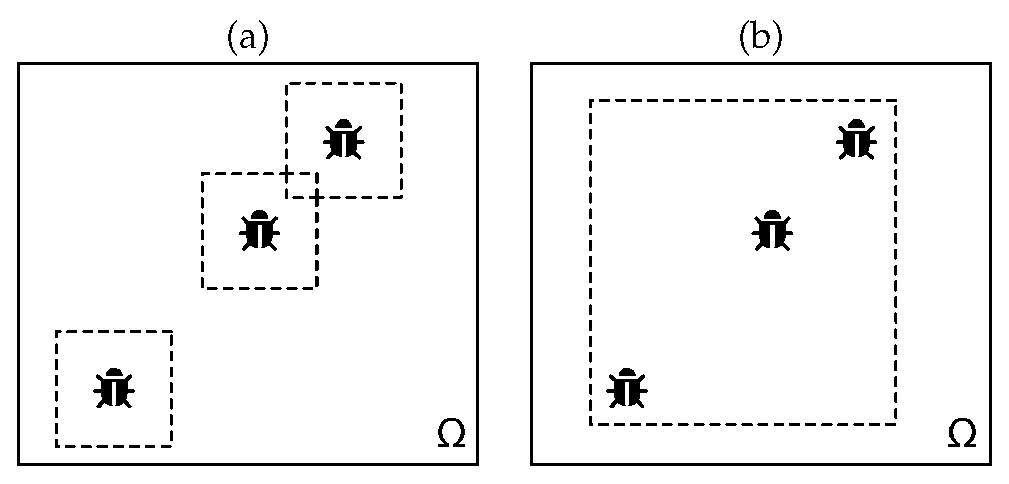
The recruitment phase was modified to limit the section of the feasible region to be searched. Originally, small search spaces were defined around each food source found during the exploration phase (Figure 2a). This was changed so that a unique subsection of the feasible region is defined. This single sub-region (Figure 2b) is defined to contain all explorers within it.

2.5. Workflow of Parallel Experiments

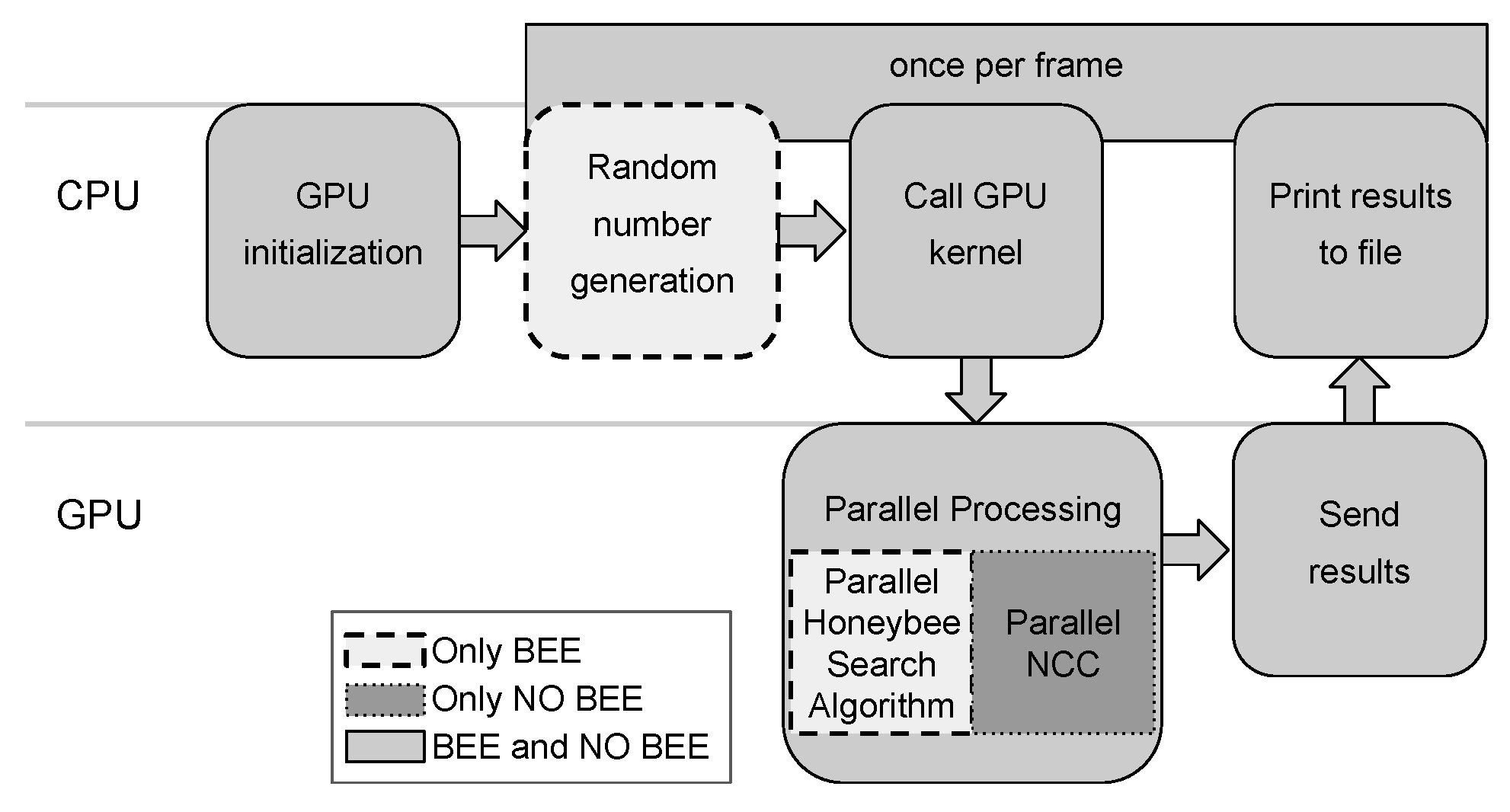
The following section provides information about several different tools that were used in conjunction to perform the experiments and evaluate the raw data that was obtained. Figure 3 shows the overall workflow. There are two main actors: the CPU and the GPU. It begins when the CPU performs operations that are required before the parallel processing is performed. Then, the GPU starts working to perform the search operations. Finally, results are sent back from the GPU to the CPU and then presented to the user.
Observe that the stage “Random number generation” (described in Section 2.5.2) is only used in program that uses HSA (BEE) because the heuristic procedure requires them. Another important note is that the stage of “Parallel Processing” changes drastically between programs. The parallel processing of program BEE uses Parallel HSA while the second program performs an exhaustive search (NO BEE), using NCC.

2.5.1. Hardware

The GPU used in most of the experiments is an AMD Radeon R9 270, and it was programmed using OpenCL. The clock speed of the GPU is of 925 MHz, and the communication with the CPU is made through a PCI Express x16 slot that transmits about 16 GB/s.
The architecture of the GPU is designed for parallel operations that require no synchronization [36]. The 1280 ALUs of the GPU can work independently, but not in a coordinated manner. If the program requires synchronization, the available resources are limited. The maximum number of synchronized work-items, also called the maximum work-group, is of 256 parallel work-items [37].
The CPU used to provide instructions to the GPU, image preprocessing, random number generation, and displaying results is a DELL XPS 8700 with an Intel Core i7-4790. The base frequency of the processor is 3.60 GHz. We use OpenCV for image manipulation. The CPU also has 15.6 GiB of RAM available.
The experiments of Section 3.7, which tested state of the art trackers, requiered a second GPU with the following characteristics: NVIDIA GeForce GTX 1050 with 640 cores and 1354MHz clock speed.

2.5.2. Random Number Generation

The processors of the GPU have a limited function set. This situation presents certain difficulties, such as the lack of native support for random number generation, required for several vital activities of HSA. The solution we implemented was to pre-generate random number arrays of different distributions with the CPU and sent them along with the frame image data to the GPU. Four arrays are generated and sent from the CPU to the GPU:
  • uniformly distributed integers (using OpenCV)
  • uniformly distributed real numbers (using OpenCV)
  • beta distribution for SBX [38,39]
  • and delta distribution for Polynomial Mutation [39].

2.5.3. GPU Kernel Parameters

The GPU kernel is the program that is executed by every work-item and can receive configuration parameters if required. In this case, we sent different configuration parameters for each program, Table 1 provides a summary.
Program BEE requires several values related to HSA. Many of the assigned parameters were optimal values found by Olague and Puente [14,15,16]. Those parameters are: η m , η c , α e / λ e , β e / λ e , γ e / λ e , α h / λ h , β h / λ h , and γ h / λ h (detailed in Section 2.2). The number of generations for the exploration phase was selected using an experiment (described in Section 3.4), the harvest phase has the half of the number of generations used for exploration.

2.5.4. Honeybee Search Algorithm Parallelization

Each honeybee is logically composed of q GPU work-items. The maximum number of individuals that can work simultaneously is p / q , where p is the maximum work-group. To take advantage of these p / q individuals, the size of populations μ e , λ e , μ h and λ h are all set to the same size of p / q .
When evaluating the fitness function, all work-items that belong to a certain individual have work to do. However, there are activities in HSA that require a lower level of parallelization and only use one processor per individual. The list of activities that fall in this category are:
  • generation of the initial random μ e population for the exploration phase
  • generation of λ populations using mutation, crossover and random exploration
  • merge μ and λ populations
  • selection of the μ best from μ + λ populations
Before the selection of the μ best from the μ + λ population, said population has to be sorted by fitness value. The sorting algorithm used in the described implementation is a parallelized merge-sort, that uses one work-item per honeybee [40].
The only phase not parallelized at all is the recruitment phase. One processor keeps working while the rest remain idle. This processor assigns how many foragers will be recruited by each explorer bee and defines the new search space.

2.6. Tests Procedure and Evaluation Criteria

The tests and evaluation of the different developed tracker proposals were carried out considering several evaluation criteria. First, the tests were performed using the ALOV video dataset (described in Section 2.6.1). Secondly, a quantitative evaluation is carried out using the F-score criterion for each proposal and analyzed using a survival curve (detailed in Section 2.6.2). Subsequently, the average time per frame criterion is obtained for each proposal and analyzed using a survival curve (detailed in Section 2.6.3). Besides, the time complexity is derived for each proposal and contrasted with the obtained results. Finally, performance in terms of accuracy and processing time for each proposal is analyzed through a proposed criterion, called Score-Time Efficiency (detailed in Section 2.6.4).

2.6.1. ALOV Video Dataset

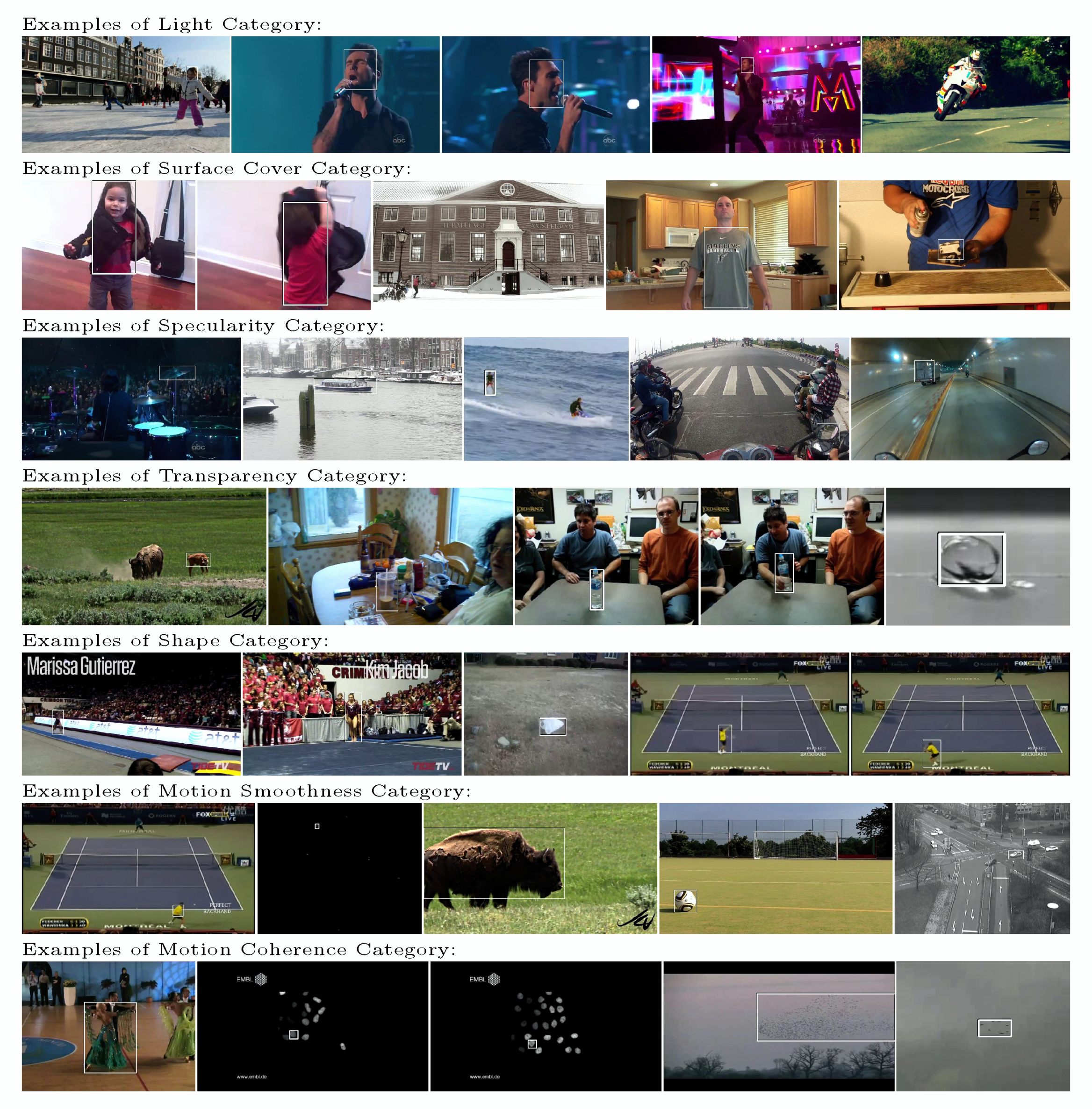
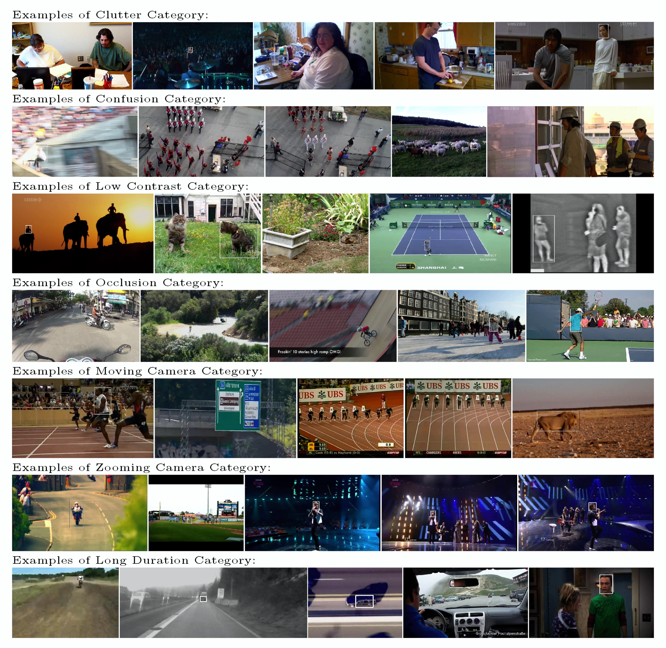
The tests were performed using the ALOV video dataset (Figure 4 and Figure 5) proposed by [3]. This dataset provides 314 videos and ground truth data for evaluation and has been used as a benchmark to test 19 different trackers.
The ALOV dataset has 14 categories and each one presents a different challenge for common trackers. The categories are:
  • Light: 33 videos that have sudden and intense changes in the main light source or how it illuminates the tracked object.
  • Surface Cover: 15 videos where the tracked object changes its surface cover, but this cover adopts the form of the object it covers.
  • Specularity: 18 videos with shiny objects that reflect light and produce specularities.
  • Transparency: 20 videos where the tracked object is transparent and easily confused with the background.
  • Shape: 24 videos in which the tracked object drastically changes its shape.
  • Motion Smoothness: 22 videos that show an object that moves so slowly that no movement is detected whatsoever.
  • Motion Coherence: 12 videos where the tracked object does not follow a predictable route of movement.
  • Clutter: 15 videos with tracked objects that display similar patterns to the ones observed in the background.
  • Confusion: 37 videos that show objects that are very similar to the object of interest, thus confusing the tracker.
  • Low Contrast: 23 videos where the tracked object shows little contrast with the background or other objects.
  • Occlusion: 34 videos where the object of interest is occluded by other objects or is not in the field of vision at a certain point.
  • Moving Camera: 22 videos that are affected by the camera’s sudden movements.
  • Zooming Camera: 29 videos where the zoom of the camera changes the displayed size of the object.
  • Long Duration: 10 videos that have greater duration, between one and two minutes.
To perform a quantitative evaluation against the other 19 trackers, the dataset authors suggest using the F-score [3], which is a measurement tool based on the intersection and union area between the provided answer and the real answer. We have successfully applied this measure to other evolutionary algorithms dealing with video tracking [6,7].
The authors of the dataset suggest the use of a survival curve; a type of graph that shows the results sorted in descending order and is more commonly used in the field of medicine to compare how different treatments affect patients [41,42]. The curves that are closer to the labeled horizontal line can be considered the most accurate.

2.6.2. F-Score

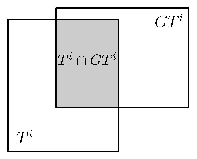
The F-score F is evaluated using Equations (14) and (15). The first Equation (14) is known as the PASCAL criterion and it helps to identify false positives and true positives. The criterion depends on how the rectangular window T i is given as a result for a certain frame (also called truth) intersects with the ground truth G T i and how this area compares to the union of both as illustrated in Figure 6. The ground truth data was also provided as part of the ALOV++ dataset to allow faster testing and measurement of new algorithms.
| T i G T i | | T i G T i | 0.5
The number of false positives n f p increases when the PASCAL criterion fails; the number of true positives n t p increases on the opposite case, and the number of false negatives n f n increases when the object is present on the frame according to the ground truth, but the tested algorithm determines the object was not detected.
p r e c i s i o n = n t p n t p + n f p r e c a l l = n t p n t p + n f n F-score = 2 · p r e c i s i o n · r e c a l l p r e c i s i o n + r e c a l l
Note F only has non-negative values lesser or equal to 1, and the PASCAL criterion measures not only that the result is in the correct place but also that it reflects the current, correct size of the tracked object.

2.6.3. Average Time per Frame

The average time per frame is obtained using the summation of the seconds used to process each frame (seconds per frame, spf) of each video sequence divided by the number of frames in that sequence.
Average Time per Frame = sec onds per frame i Number of frames
The average time per frame should be obtained for each video of the dataset and each one of the different tracker proposals. We also used the survival curve plots to visualize the average time per frame data. Moreover, the time complexity is formally detailed and later confirmed with experimental results.

2.6.4. Score-Time Efficiency

To allow the comparison in terms of F-score and seconds per frame, this work proposes the Score-Time Efficiency. This rate describes how much benefit is obtained in terms of F-score by each second spent to process the frame. The tracker proposal with the greater Score-Time Efficiency will be considered better. Equation (17) shows how we obtained the Score-Time Efficiency.
Score-Time Efficiency = F-score Average Time per Frame

3. Results

The Big O notation or asymptotic notation is used in the literature to describe the running time of algorithms [43]; this work uses it with to predict how a certain proposed tracker would compare against another one and how parallelization affects its performance in an abstract and formal manner (see Section 3.1). The theoretical analysis is later confirmed by experimental evidence.
Section 3.2 observes the difference between using CPU or GPU to process exhaustive NCC. To continue, our NCC implementation is validated and compared to other trackers using the results reported by Smeulders et al. [3] (Section 3.3). Later, Section 3.4 describes the experiment that was performed to find the optimal number of generations for HSA. Ultimately, the experiment in Section 3.5 determines which of the proposed implementations is the best alternative in terms of accuracy and speed. Additionally, Section 3.6 uses artificial noise to test the robustness of the best alternative. Finally, Section 3.7 provides the comparison of the performance of our best alternative against other recent trackers.

3.1. Polynomial Time Complexity

The time complexity of NCC is obtained by observing Equations (11), (12) and (13). The time it takes to get t ¯ using Equation (13) is of O ( m × n ) . The next term I ¯ u , v is also obtained in a time of O ( m × n ) . Finally, γ ( u , v ) is computed using three different summations, each of them require O ( m × n ) . To conclude, the time complexity of computing γ ( u , v ) for a single point ( u , v ) is O ( m × n ) .
Sequential exhaustive NCC requires to compute every single possible γ ( u , v ) for every ( u , v ) . This is the size of the feasible region ( w m ) × ( h n ) . So O ( m × n ) × O ( ( w m ) × ( h n ) ) = O ( m 2 n h + m n w h + m 2 n 2 m n 2 w ) = O ( m n w h ) , note that m n w h is the greatest term because m should be smaller or equal to w and n should be lesser or equal to h (as illustrated in Figure 1). This is the time complexity of sequential exhaustive NCC (Table 2 row 1).
In exhaustive parallel NCC, the GPU performs the computation of several γ ( u , v ) simultaneously. Let c be the maximum number of simultaneous work-items of the GPU, then the time complexity of parallel exhaustive NCC is O ( m n w h c ) (Table 2 row 2).
HSA time complexity can be obtained observing the pseudocode in Figure 1, Figure 2 and Figure 3; and Equations (1) and (2). Please note that this analysis is specific to the case where the fitness function is γ ( u , v ) , if the fitness function experiences any change, then so does the time complexity. The first line of the Exploration pseudocode takes O ( μ e ) , as it is a constrained random generation of μ e individuals. The second line of the exploration pseudocode has a time complexity of O ( μ e m n ) since γ ( u , v ) is computed for every one of the μ e individuals. Next, the time for line 4 is of O ( λ e ) and O ( λ e m n ) for line 5; line 6 is omitted (no sharing). Exploration line 7 performs sorting, taking O ( ( μ e + λ e ) log ( μ e + λ e ) ) . In total, lines 4–7 have a time complexity of O ( λ e m n ) , since line 5 should be significantly slower to compute. This O ( λ e m n ) time complexity operation is repeated several times (line 3), this number is called the maximum number of generations or g, producing a time complexity of O ( g λ e m n ) which is polynomially greater than the cost of lines 1–2. Thus, the exploration phase takes O ( g λ e m n ) . The recruitment phase requires the summation of the fitness of all the μ e individuals (Equation (1)) and then Equation (2) has to be computed for each of those individuals, producing a time complexity of O ( μ e ) . The harvest phase is very similar to the exploration phase; the key difference is the size of the evaluated populations ( μ h and λ h ) resulting in time complexity of O ( g λ h m n ) . In polynomial terms, the greatest time complexity between exploration, recruitment, and harvest phases is that of the harvest phase given that it should be true that λ h > λ e ; taking those considerations the time complexity for sequential HSA NCC (Table 2 row 3) is of O ( g λ h m n ) time complexity.
The parallelization of HSA is described in Section 2.5.4. The evaluation of the fitness function γ ( u , v ) for each individual is performed by q work-items simultaneously. Please note that all individuals are processed in parallel because the number of individuals is p / q , and this is dependent on the capacity of the GPU. This step derives in a O ( m n q ) time complexity to get the fitness of all individuals in the population once. Still, it is not possible to process several generations at the same time; they are dependent on the results of the previous generation. Thus, the overall time complexity of Parallel HSA NCC (Table 2 row 4) is O ( g m n q ) .
It is clear that O ( m n w h ) > O ( m n w h c ) and O ( g λ h m n ) > O ( g m n q ) , then the parallelization is expected to successfully accelerate computations in both cases. However, the comparison between using exhaustive search or using HSA is non-intuitive. Still, we could reduce it to the simple idea that HSA will be faster if the size of the image frame ( w × h ) is significantly greater than the number of individuals in the λ h population multiplied by the number of generations g. In summary, HSA is expected to be faster than exhaustive search as long as w h > g λ h , which should be the case in most if not all of the tested videos. In the following sections, the different tracker proposals are tested in terms of speed and accuracy, to contrast the time complexity derivations of each proposal, and to confirm the advantages of parallelizing HSA for object tracking.

3.2. Sequential Exhaustive NCC vs. Parallel Exhaustive NCC

Our theoretical analysis has supported the assumption that using a GPU produces an acceleration against using the CPU to compute NCC with an exhaustive search. The experiments show that the assumption is correct, the GPU implementation of exhaustive NCC takes fewer seconds per frame on average.
We considered impractical to fully process all videos of the ALOV dataset using the CPU and exhaustive search, but in order to estimate the average time per frame, we tested the first two frames of each video. We made this decision because the CPU required 1 day and 18 h to process the first 5 videos of the ALOV dataset. To check that the accuracy of the results is not affected, a few random videos from the ALOV dataset were selected and used for testing, According to the results (Table 3), the GPU computes NCC for a full frame around 170 times faster than the CPU. A small difference was observed in the average F-score, equivalent to 12.60% of the overall standard deviation (not relevant).
As expected, the parallelization of exhaustive NCC successfully accelerated the execution. This result supports our previous time complexity analysis: O ( m n w h ) > O ( m n w h c ) .

3.3. Reported NCC and Other Trackers versus This Work’s NCC

This experiment was performed to show that the proposed NCC implementation behaves as reported by other authors. We used all the 314 videos of the ALOV dataset for testing in this experiment. The tests labeled OURS use the described GPU implementation of NCC and the tests labeled CTRL are the ones reported for NCC [3,44].
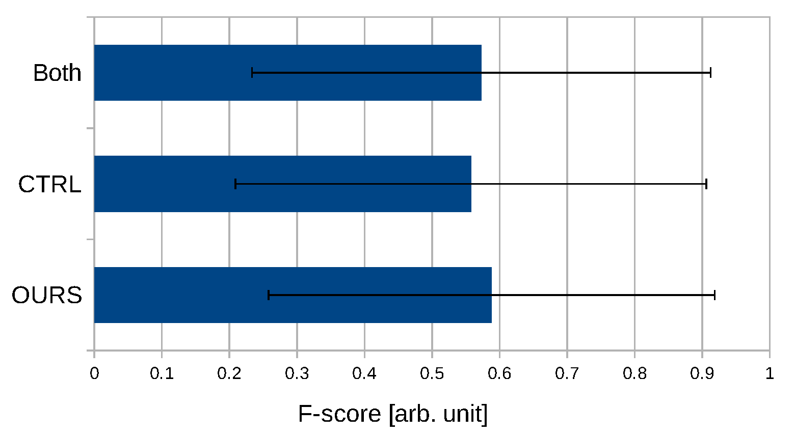
As illustrated in Figure 7, the difference in average F-score between OURS and CTRL is small. The distance between the averages is 9.06% of the standard deviation of all the tests, not significant. These results validate that the proposed GPU implementation of NCC performs as good as expected in terms of F-score.
Figure 8 shows survival curves for OURS, CTRL and 18 trackers reported by Puddu [44]. Survival curves are obtained by sorting the scores for every video and show a general overview of the video tracker performance; the closer the curve is to the perfect score (1.0), the better. The other trackers that are displayed are: Struck (STR) [45], Foreground-Background Tracker (FBT) [46], Tracking Learning and Detection (TLD) [47], Tracking by Sampling Trackers (TST) [48], Lucas-Kanade Tracker (LKT) [49], Kalman Appearance Tracker (KAT) [50], Fragments-based Robust Tracking (FRT) [51], Mean Shift Tracking (MST) [52], Locally Orderless Tracking (LOT) [53], Incremental Visual Tracking (IVT) [54], Tracking on the Affine Group (TAG) [55], Tracking by Monte Carlo (TMC) [56], Adaptive Coupled-layer Tracking (ACT) [57], 1 -minimization Tracker (L1T) [58], 1 Tracker with Occlusion detection (L1O) [59], Hough-Based Tracking (HBT) [60], Super Pixel tracking (SPT) [61], and Multiple Instance learning Tracking (MIT) [62].
According to this experiment, our implementation of NCC is validated and can be considered a tracker of acceptable performance in terms of accuracy.

3.4. Adjusting the Honeybee Search Algorithm

This experiment was designed to determine if the time per frame is reduced when the number of generations (explained in Section 2.2) is lower, and what is the optimal number of generations. This experiment considers all the 314 videos of the ALOV dataset. All the tests use NCC, GPU, and HSA. The variation is made in the number of generations. The other configuration parameters of HSA reuse optimal values proposed by Olague and Puente [14,15,16] after numerous experiments.
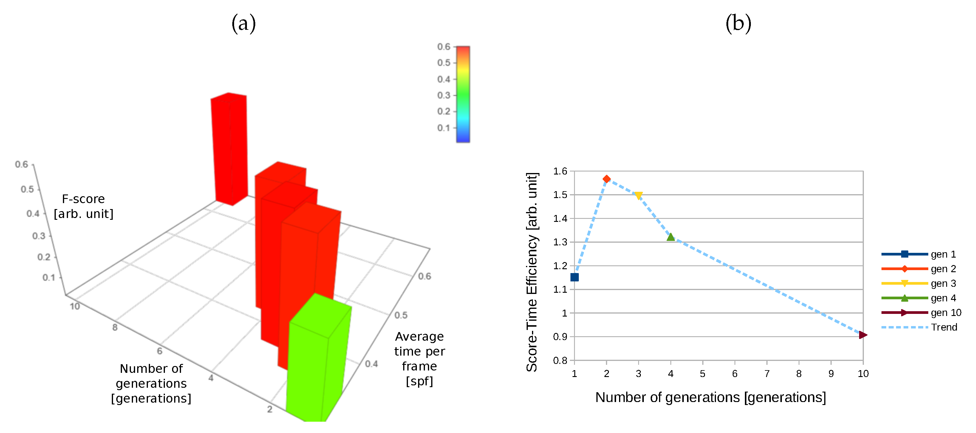
Figure 9a shows that the average F-score is stable between generations 2 to 10. The difference in score between 2 and 3 generations is 3.50% of the overall standard deviation, and 1.95% between 3 and 4 generations. The leap between 4 and 10 generations is only of 4.02%. On the other hand, there is a notable difference between 1 and 2 generations, measured as 66.79% of the overall standard deviation.
Figure 9b shows that as the number of generations increases, the average time per frame increases. From 1 to 2 generations, the average time per frame increases by 8.65% of the overall standard deviation. From 2 to 3 generations, the increment is 4.50%. When changing from 3 to 4 generations, time per frame increases by 8.48%. The pattern is caused by the increment in the number of generations for the harvest phase, which is the half of the generations used for the exploration phase. Finally, an increment from 4 to 10 generations causes the average time per frame to increase by 38.82% of the overall standard deviation, showing that the trend continues.
Figure 10a shows a three-dimensional plot, the axes show the average F-score, the average time per frame and the number of generations; the color of the bars indicates a difference in the average F-score; this helps to visualize the trend observed when the number of generations of HSA varies. After two generations, the average F-score stabilizes. In contrast, the average time per frame keeps increasing. We inferred from that information that two generations provide the right balance between time and score. Nevertheless, the Score-Time Efficiency shows without a doubt that two generations is the best option (Figure 10b).
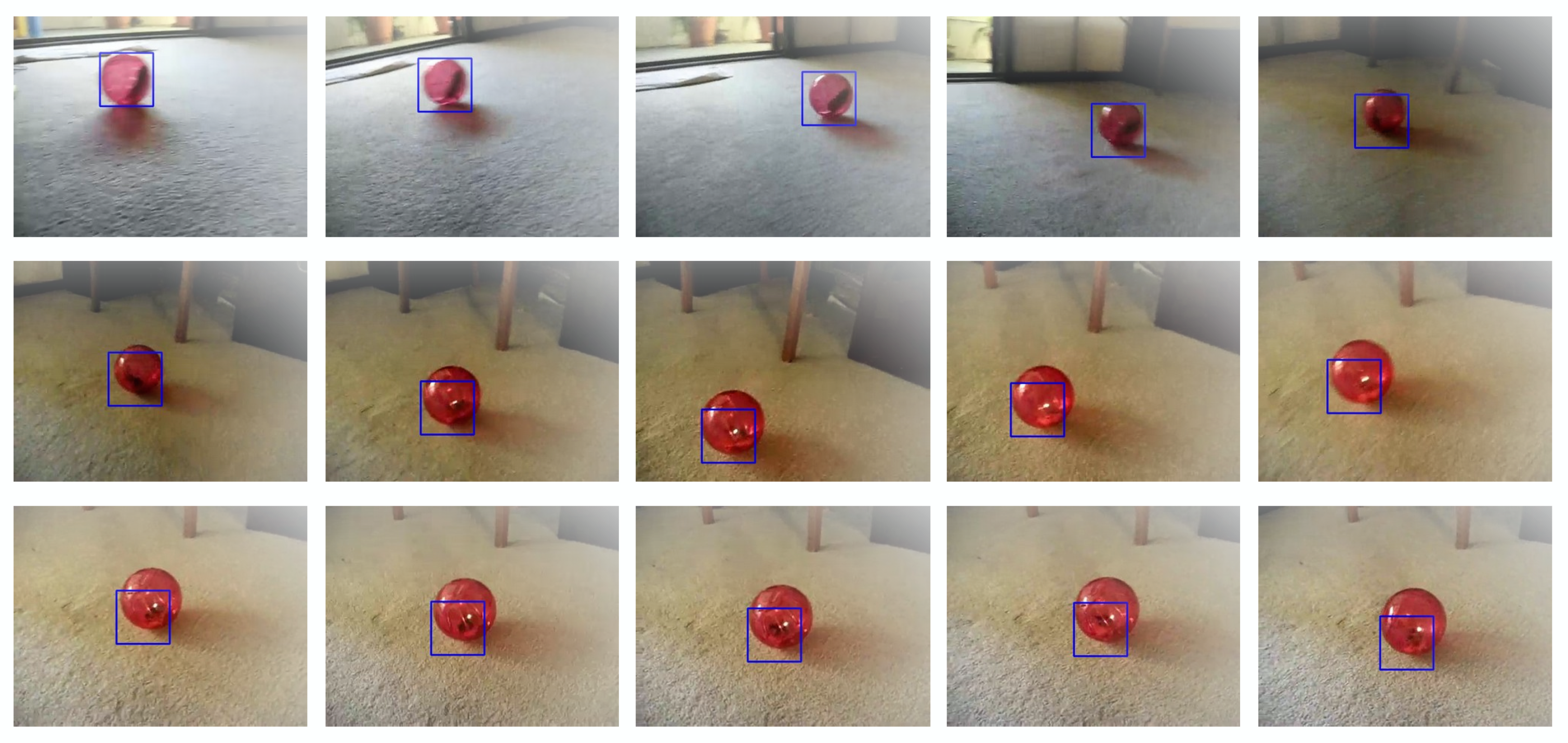
As expected, the average time increases with each new generation. This aspect supports the time complexity analysis of parallel HSA with NCC as fitness function: O ( g m n q ) , where the number of generations is of significant influence. This result shows the practical utility of the Score-Time Efficiency, using it to determine that the optimal number of generations. Also, the observation that the F-score has asymptotic behaviour starting on two generations ensures that selecting that number does not mean a negative effect on accuracy. Figure 11 shows an example of the results that were obtained using two generations, the location of the object (a ball) is obtained with a certain degree of accuracy even when the size and illumitation of the object changes.

3.5. GPU Exhaustive vs. GPU with Honeybee Search Algorithm

This experiment also uses all the 314 videos of the ALOV dataset and all the tests use NCC and the GPU. The tests labeled BEE use Parallel HSA configured to run for two generations, and the ones labeled NO BEE use exhaustive search. Keep in mind that the full capacity of the GPU is not used in BEE because of the synchronization needs.
Notice in Figure 12 that the average difference of F-score between BEE and NO BEE is relatively small. This difference is 1.54% of the overall standard deviation, an irrelevant difference. This validates that BEE performs as good as the exhaustive NCC tracker.
The difference of average time per frame, displayed in Figure 13a, is of 42.22% of the overall standard deviation. However, there is a remarkable difference in the standard deviation of both groups. In other words, BEE provides a lower and more stable time per frame (about 7.58 times steadier). This result validates that using Parallel HSA provides an improvement in time per frame against a plain GPU-accelerated NCC. Figure 13b shows how using the GPU accelerates the implementation that uses HSA and how it compares against exhaustive search. This outcome shows how the polynomial time complexity of GPU BEE is lower than GPU NO BEE, which is lower than CPU NO BEE, supporting the theoretical analysis O ( m n w h ) > O ( m n w h c ) > O ( g m n q ) .
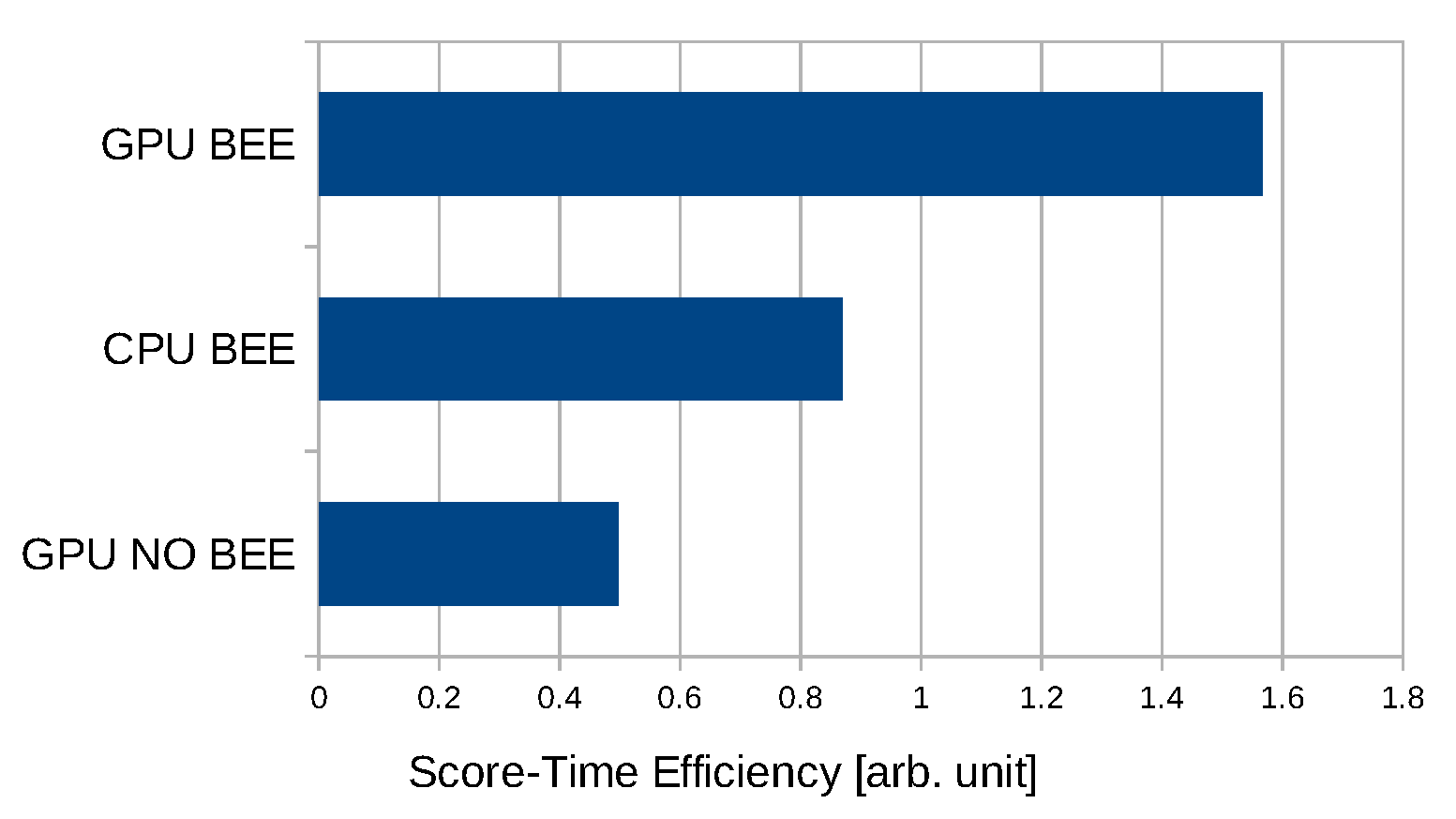
Finally, Figure 14 shows that using parallel HSA (GPU BEE) provides a greater Score-Time Efficiency meaning it is the best alternative. This simple observation is an intuitive condensation of the previous analysis of both the F-score and average time per frame observations.

3.6. Tests with Gaussian Noise

This experiment uses 14 videos of the ALOV dataset, one for each category. All the tests use NCC, HSA with two generations, and GPU. We apply Gaussian noise to test the resistance of the proposal to external perturbations. Gaussian noise requires the configuration parameters of median and standard deviation to generate random numbers with that distrubution [63], and then these are added to the values of each color channel. Figure 15 shows an example frame without noise (a), this is labeled as noise level 0. Then, the same frame with Gaussian noise using median and standard deviation with a noise level of 50 shown in (b). Finally, the same example frame with Gaussian noise using median and standard deviation with a noise level of 100 shown in (c).
The Figure 16a shows that there is a difference in F-score between videos that display different levels of noise. In other words, the underlying object tracker (NCC) shows a degree susceptibility to noisy image frames. The difference between noise level 0 and level 50 is 34.88% of the overall standard deviation, and the difference between levels 50 and 100 is of 10.38% of the total standard deviation. On the other hand, Figure 16b shows that noise has no noticeable effect on the average time per frame.
A conclusion drew from the results obtained with the combination of NCC, HSA with two generations, and GPU is that Gaussian noise affects the accuracy. Nevertheless, the difference in F-score observed between no noise (level 0), and some noise (50 and 100) is in the range of 0.11 to 0.14, which is small considering that the full range of the F-score is from 0 to 1. On the other hand, the noise has no effect on speed.

3.7. Our Best Tracker Proposal versus Two Recent Trackers

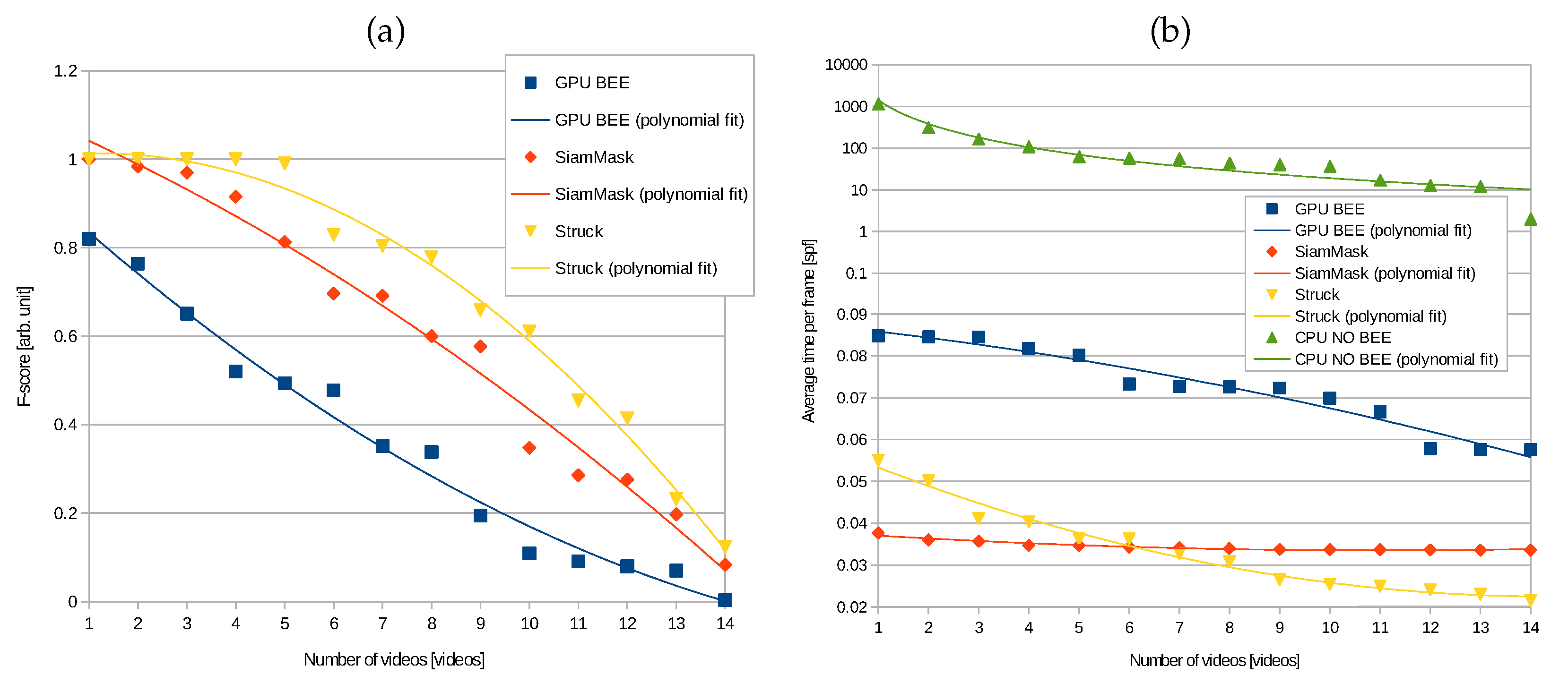
Two different recent trackers were selected for contrast: Struck [45] and SiamMask [10]. Struck remains relevant because it is a purely online tracking proposal that requires no kind of training and is still able to participate in the latest issues of the VOT challenge [64]. On the other hand, SiamMask is considered among the best tracker proposals that participated in the latest VOT challenge (top 20) in terms of accuracy, also several techniques that take inspiration from SiamMask are positioned in the toptier. SiamMask relies on pre trainined models as it is based on convolutional neural networks. This section compares the performance of this two state of the art trackers against our best proposal (GPU BEE) in terms of speed and accuracy using 14 videos of the ALOV dataset, one per category.
The analysis of Struck and SiamMask revealed that both trackers preprocess the image frames before actually performing tracking, in the case of SiamMask this is usefull to reduce latency caused by the CPU to GPU communication. Taking that into account, a simple reduction of the frame size is performed in our proposal, by scaling the picture accordingly, whenever the width or the height of the frame is greater than 300 pixels. The effect on the accuracy caused by the reduction of frames can be considered negligible compared to the full resolution frame. On the other hand, a relevant reduction of the average time per frame is obtained.
Figure 17a shows that the accuracy of GPU BEE is inferior to that of SiamMask and Struck. This is not surprising since GPU BEE uses NCC as a tracker, and different sources have found it to be surpassed in accuracy by Struck. However it is interesting to note that Struck showed a better accuracy than SiamMask in this particular setting, which is not the general case. The conclusion that is drawn is that Struck shows greater robustness in certain cases: low resolution videos and videos with background objects that resemble the target. In addition, it is clear that the parallelization of the HSA does not improve the accuracy of its fitness function (Figure 13), but a significant acceleration is observed compared to the conventional NCC tracker. As shown in (Figure 17b), the average time per frame of our best proposal (GPU BEE) is almost four orders of magnitude smaller than that obtained for CPU NO BEE. Moreover, the survival curve of average time per frame of GPU BEE is in the same window (from 0.2 to 0.9 spf) of Struck and SiamMask, a remarkable improvement against CPU NO BEE.

4. Discussion

The main concern of this work is to find out whether our proposed combination of HSA and GPU is capable of accelerating a given object tracker. It is shown in Figure 12 and Figure 13 that the optimal proposal, the one that maximizes accuracy and speed, is parallel HSA. An area of opportunity that arises from this work is whether or not parallel HSA using NCC as fitness function can compete against other trackers in terms of speed. During the tests combining the GPU, HSA, and NCC, the minimum observed latency was of 0.0351 s per frame; the maximum was 2.6715 s per frame; and the average was of 0.3729 s per frame. The results show that the tracker’s speed is affected by the dimensions of the frame (width and height); as well as the size of the tracked object.
We reviewed the literature and found that the ALOV dataset was not used to test the speed of trackers due to the authors’ emphasis on accuracy. On the other hand, the dataset presents a demanding task because the frame sizes that range from 192 × 144 to 1920 × 1080 pixels and post many different challenges. Other authors have reported speed of their tracker proposals. For example, Wu et al. [4] which used video sequences with frame sizes than range from 128 × 96 to 640 × 480 pixels, which are significantly smaller than ALOV frame sizes. Using the data of the most accurate trackers reported in that benchmark [4], we found that the minimal latency is of 0.0027 s per frame, the maximum latency is of 1.9607 s per frame and the average is 0.3228 s per frame. In contrast our average time (0.3729 s per frame) seems to fall on the average, despite the fact that the ALOV dataset has larger frame sizes and presents more complex challenges.
This work presents the results of tests using only one object tracker (NCC), but the parallelized version of the Honeybee Search Algorithm as presented could and ought to be combined with other object trackers. This combination can provide more evidence of the benefits of combining these tools. Testing with other object trackers is not a trivial undertaking since this requires the study and understanding of the tracker and an analysis to determine if it can be accurately translated into a fitness function. We believe the main objective of this work has been fulfilled by providing the proof that the combination of HSA and the GPU is useful to accelerate the NCC object tracker without adverse effects on its accuracy. For future work, we have decided to address this further by testing this configuration with other trackers (Section 5.1). Another relevant point that supports the previous observation is that the parallel HSA was capable of accelerating NCC to the point of reaching Struck and SiamMask speed levels even when NCC is not a state of the art tracker as is confirmed in Section 3.7.
According to our results, the GPU may not be the best tool for the parallelization of HSA or other Swarm Intelligence algorithms. The GPU was designed to perform vector operations with small synchronization requirements, while many Swarm Intelligence algorithms focus on the idea of synchronization of individuals. Usually, a GPU has a limit to the number of possible synchronized threads, often a fraction of the full capacity of the GPU. Nevertheless, our parallel implementation of HSA achieved a higher speed than naïve parallelization of the NCC tracker. Even though, the used hardware is not the best alternative in the market, we found that our parallelization approach enhances the performance of the NCC tracker and this should be translatable to another GPU with higher capacities.

5. Conclusions

The presented results provide evidence to conclude that the proposed combination of a GPU and HSA can be useful to accelerate NCC, and possibly other trackers. Furthermore, using HSA, together with the GPU, provides a greater acceleration than using the GPU alone. Even when HSA is not a deterministic tool, the accuracy is not negatively affected when using it.
The experiments helped find the optimal value for the number of generations (two generations), an important configuration parameter for HSA that has an effect in speed and accuracy. Both the time complexity analysis and the experimental evidence showed the extent of the influence that this parameter has in the tracker’s execution speed. Other experiments showed that the proposal is resistant to high levels of noise.
The proposed Score-Time Efficiency criterion was found useful to make simple comparisons of different tracker proposals in terms of accuracy and speed, allowing making decisions that require the optimization of both variables. According to the analysis performed using this criterion, the best option was parallel HSA with 2 generations using NCC as fitness function.
Comparison experiments of our best proposal against other recent trackers such as SiamMask and Struck show evidence that parallel HSA has no relevant effects on the accuracy of its tracker function (NCC), but dramatically reduces latency, almost four orders of magnitude in terms of average time per frame. This evidence exposes an opportunity area in which to focus future efforts: to employ the proposed methodology but using state of the art trackers as a starting point.

5.1. Future Work

  • Perform tests with different datasets. Since the ALOV dataset is mainly focused on accuracy. An interesting dataset could be the object tracking benchmark of Kristan et al. [64]. Also, use state-of-the-art trackers and other well-known traditional trackers for testing. For instance, Struck [45] and SiamMask [10] are currently considered some of the most accurate and fast trackers [3,64].
  • Perform tests with different parallel computing or hardware acceleration technologies. The synchronization required by HSA could be provided by another architecture such as the FPGA [65], which would allow designing a parallel computing architecture with custom capabilities.
  • Comparisons with other Swarm Intelligence heuristics. This work used HSA, which could be compared against other similar heuristics, such as Particle Swarm Optimization or Artificial Bee Colony.

Author Contributions

Conceptualization, O.E.P.-C. and C.P.; Methodology, C.S.-M. and C.P.; Formal analysis, C.S.-M., G.O. and C.A.A.-S.; Investigation, O.E.P.-C. and C.P.; Validation, C.S.-M., G.O. and C.A.A.-S.; Data curation, O.E.P.-C. and A.S.N.-V.; Software, O.E.P.-C., C.P. and A.S.N.-V.; Writing—original draft preparation, O.E.P.-C., C.S.-M. and C.P.; Writing—review and editing, G.O., C.A.A.-S. and A.S.N.-V. All authors have read and agreed to the published version of the manuscript.

Funding

This research was funded by CONACYT grant number 25096. Also, this research was partially supported by CONACYT, through the project CB-2012/177041.

Acknowledgments

The authors especially wish to thank José de Jesús Díaz for his English usage suggestions to improve the writing of the article.

Conflicts of Interest

The authors declare no conflict of interest.

References

  1. Roy, A.; Chattopadhyay, P.; Sural, S.; Mukherjee, J.; Rigoll, G. Modelling, synthesis and characterisation of occlusion in videos. IET Comput. Vis. 2015, 9, 821–830. [Google Scholar] [CrossRef]
  2. Tesfaye, Y.T.; Zemene, E.; Pelillo, M.; Prati, A. Multi-object tracking using dominant sets. IET Comput. Vis. 2016, 10, 289–298. [Google Scholar] [CrossRef]
  3. Smeulders, A.W.; Chu, D.M.; Cucchiara, R.; Calderara, S.; Dehghan, A.; Shah, M. Visual tracking: An experimental survey. IEEE Trans. Pattern Anal. Mach. Intell. 2014, 36, 1442–1468. [Google Scholar]
  4. Wu, Y.; Lim, J.; Yang, M.H. Object tracking benchmark. IEEE Trans. Pattern Anal. Mach. Intell. 2015, 37, 1834–1848. [Google Scholar] [CrossRef] [PubMed] [Green Version]
  5. Galoogahi, H.K.; Fagg, A.; Huang, C.; Ramanan, D.; Lucey, S. Need for speed: A benchmark for higher frame rate object tracking. In Proceedings of the IEEE International Conference on Computer Vision (ICCV), Venice, Italy, 22–29 October 2017; IEEE: Hoboken, NJ, USA, 2017; pp. 1134–1143. [Google Scholar]
  6. Olague, G.; Hernández, D.E.; Llamas, P.; Clemente, E.; Briseño, J.L. Brain programming as a new strategy to create visual routines for object tracking. Multimed. Tools Appl. 2019, 78, 5881–5918. [Google Scholar] [CrossRef]
  7. Olague, G.; Hernández, D.E.; Clemente, E.; Chan-Ley, M. Evolving Head Tracking Routines With Brain Programming. IEEE Access 2018, 6, 26254–26270. [Google Scholar] [CrossRef]
  8. Yazdi, M.; Bouwmans, T. New trends on moving object detection in video images captured by a moving camera: A survey. Comput. Sci. Rev. 2018, 28, 157–177. [Google Scholar] [CrossRef]
  9. Björkman, M.; Bergström, N.; Kragic, D. Detecting, segmenting and tracking unknown objects using multi-label MRF inference. Comput. Vis. Image Underst. 2014, 118, 111–127. [Google Scholar] [CrossRef] [Green Version]
  10. Wang, Q.; Zhang, L.; Bertinetto, L.; Hu, W.; Torr, P.H. Fast online object tracking and segmentation: A unifying approach. In Proceedings of the IEEE Conference on Computer Vision and Pattern Recognition, Long Beach, CA, USA, 15–20 June 2019; pp. 1328–1338. [Google Scholar]
  11. Lu, S.; Yu, X.; Li, R.; Zong, Y.; Wan, M. Passive cavitation mapping using dual apodization with cross-correlation in ultrasound therapy monitoring. Ultrason. Sonochem. 2019, 54, 18–31. [Google Scholar] [CrossRef]
  12. Yang, X.; Deka, S.; Righetti, R. A hybrid CPU-GPGPU approach for real-time elastography. IEEE Trans. Ultrason. Ferroelectr. Freq. Control 2011, 58, 2631–2645. [Google Scholar] [CrossRef]
  13. Idzenga, T.; Gaburov, E.; Vermin, W.; Menssen, J.; De Korte, C.L. Fast 2-D ultrasound strain imaging: The benefits of using a GPU. IEEE Trans. Ultrason. Ferroelectr. Freq. Control 2014, 61, 207–213. [Google Scholar] [CrossRef] [PubMed]
  14. Olague, G.; Puente, C. The honeybee search algorithm for three-dimensional reconstruction. In Proceedings of the Workshop on Applications of Evolutionary Computation, Budapest, Hungary, 10–12 April 2006; Springer: Berlin/Heidelberg, Germany, 2006; pp. 427–437. [Google Scholar]
  15. Olague, G.; Puente, C. Parisian evolution with honeybees for three-dimensional reconstruction. In Proceedings of the 8th Annual Conference on Genetic and Evolutionary Computation, Seattle, WA, USA, 8–12 July 2006; ACM: New York, NY, USA, 2006; pp. 191–198. [Google Scholar] [CrossRef]
  16. Olague, G.; Puente, C. Honeybees as an intelligent based approach for 3D reconstruction. In Proceedings of the 18th International Conference on Pattern Recognition (ICPR’06), Hong Kong, China, 20–24 August 2006; IEEE: Hoboken, NJ, USA, 2006; Volume 1, pp. 1116–1119. [Google Scholar] [CrossRef] [Green Version]
  17. Olague, G. Evolutionary Computer Vision: The First Footprints; Springer: Berlin/Heidelberg, Germany, 2016. [Google Scholar]
  18. Simonite, T. Virtual Bees Help Robots See in 3D. Available online: https://www.google.com.mx/amp/s/www.newscientist.com/article/dn10129-virtual-bees-help-robots-see-in-3d/amp/ (accessed on 20 December 2019).
  19. Tan, Y.; Ding, K. A survey on GPU-based implementation of swarm intelligence algorithms. IEEE Trans. Cybern. 2016, 46, 2028–2041. [Google Scholar] [CrossRef] [PubMed]
  20. Kalivarapu, V.; Winer, E. Implementation of digital pheromones in PSO accelerated by commodity graphics hardware. In Proceedings of the 12th AIAA/ISSMO Multidisciplinary Analysis and Optimization Conference, Victoria, BC, Canada, 10–12 September 2008; pp. 1–17. [Google Scholar]
  21. Hsieh, H.T.; Chu, C.H. Particle swarm optimisation (PSO)-based tool path planning for 5-axis flank milling accelerated by graphics processing unit (GPU). Int. J. Comput. Integr. Manuf. 2011, 24, 676–687. [Google Scholar] [CrossRef]
  22. Tsutsui, S.; Fujimoto, N. ACO with tabu search on a GPU for solving QAPs using move-cost adjusted thread assignment. In Proceedings of the 13th Annual Conference on Genetic and Evolutionary Computation, Dublin, Ireland, 12–16 July 2011; ACM: New York, NY, USA, 2011; pp. 1547–1554. [Google Scholar]
  23. Calazan, R.M.; Nedjah, N.; de Macedo Mourelle, L. Three alternatives for parallel GPU-based implementations of high performance particle swarm optimization. In Proceedings of the International Work-Conference on Artificial Neural Networks, Puerto de la Cruz, Tenerife, Spain, 12–14 June 2013; Springe: Berlin/Heidelberg, Germany, 2013; pp. 241–252. [Google Scholar]
  24. Souza, D.L.; Teixeira, O.N.; Monteiro, D.C.; de Oliveira, R.C.L. A new cooperative evolutionary multi-swarm optimizer algorithm based on CUDA parallel architecture applied to solve engineering optimization problems. In Proceedings of the 3rd International Workshop on Combinations of Intelligent Methods and Applications (CIMA 2012), Montpellier, France, 27–31 August 2012; p. 49. [Google Scholar]
  25. Rohilla, R.; Sikri, V.; Kapoor, R. Spider monkey optimisation assisted particle filter for robust object tracking. IET Comput. Vis. 2016, 11, 207–219. [Google Scholar] [CrossRef]
  26. Naiel, M.A.; Ahmad, M.O.; Swamy, M.; Lim, J.; Yang, M.H. Online multi-object tracking via robust collaborative model and sample selection. Comput. Vis. Image Underst. 2017, 154, 94–107. [Google Scholar] [CrossRef]
  27. Kang, K.; Bae, C.; Yeung, H.W.F.; Chung, Y.Y. A hybrid gravitational search algorithm with swarm intelligence and deep convolutional feature for object tracking optimization. Appl. Soft Comput. 2018, 66, 319–329. [Google Scholar] [CrossRef]
  28. Crist, E. Can an insect speak? The case of the honeybee dance language. Soc. Stud. Sci. 2004, 34, 7–43. [Google Scholar] [CrossRef] [Green Version]
  29. Deb, K.; Beyer, H.G. Self-adaptive genetic algorithms with simulated binary crossover. Evol. Comput. 2001, 9, 197–221. [Google Scholar] [CrossRef]
  30. Boumaza, A.M.; Louchet, J. Dynamic flies: Using real-time parisian evolution in robotics. In Proceedings of the Workshop on Applications of Evolutionary Computation, Como, Italy, 18–20 April 2011; Springer: Berlin/Heidelberg, Germany, 2001; pp. 288–297. [Google Scholar]
  31. Goldberg, D.E.; Richardson, J. Genetic algorithms with sharing for multimodal function optimization. In Genetic Algorithms and Their Applications: Proceedings of the Second International Conference on Genetic Algorithms; Lawrence Erlbaum: Hillsdale, NJ, USA, 1987; pp. 41–49. [Google Scholar]
  32. Deb, K. Multi-Objective Optimization Using Evolutionary Algorithms; John Wiley & Sons: Hoboken, NJ, USA, 2001; Volume 16. [Google Scholar]
  33. Lewis, J.P. Fast Normalized Cross-Correlation; Vision Interface: Quebec, QC, Canada, 1995; Volume 10, pp. 120–123. [Google Scholar]
  34. Di Stefano, L.; Mattoccia, S.; Tombari, F. ZNCC-based template matching using bounded partial correlation. Pattern Recognit. Lett. 2005, 26, 2129–2134. [Google Scholar] [CrossRef]
  35. Bätz, M.; Richter, T.; Garbas, J.U.; Papst, A.; Seiler, J.; Kaup, A. High dynamic range video reconstruction from a stereo camera setup. Signal Process. Image Commun. 2014, 29, 191–202. [Google Scholar] [CrossRef]
  36. Mantour, M. AMD Radeon HD 7970 with graphics core next (GCN) architecture. In Proceedings of the Hot Chips 24 Symposium (HCS), Cupertino, CA, USA, 27–29 August 2012; pp. 1–35. [Google Scholar]
  37. Gaster, B.; Howes, L.; Kaeli, D.R.; Mistry, P.; Schaa, D. Heterogeneous Computing with OpenCL: Revised OpenCL 1; Newnes; Morgan Kaufman: San Francisco, CA, USA, 2012. [Google Scholar]
  38. Deb, K. Multi-Objective Optimization using Evolutionary Algorithms; John Wiley & Sons: Hoboken, NJ, USA, 2001. [Google Scholar]
  39. Khare, V.; Yao, X.; Deb, K. Performance scaling of multi-objective evolutionary algorithms. In Evolutionary Multi-Criterion Optimization; Springer: Berlin/Heidelberg, Germany, 2003; p. 72. [Google Scholar]
  40. Davidson, A.; Tarjan, D.; Garland, M.; Owens, J.D. Efficient parallel merge sort for fixed and variable length keys. In Proceedings of the Innovative Parallel Computing (InPar), San Jose, CA, USA, 13–14 May 2012; pp. 1–9. [Google Scholar]
  41. Lawless, J.F. Statistical Models and Methods for Lifetime Data; John Wiley & Sons: Hoboken, NJ, USA, 2011; Volume 362. [Google Scholar]
  42. Collett, D. Modelling Survival Data in Medical Research; CRC Press: Boca Raton, FL, USA, 2015. [Google Scholar]
  43. Cormen, T.H.; Leiserson, C.E.; Rivest, R.L.; Stein, C. Introduction to Algorithms; MIT Press: Boston, MA, USA, 2009. [Google Scholar]
  44. Puddu, L. ALOV300++ Dataset. Available online: http://alov300pp.joomlafree.it/ (accessed on 20 December 2019).
  45. Hare, S.; Golodetz, S.; Saffari, A.; Vineet, V.; Cheng, M.M.; Hicks, S.L.; Torr, P.H. Struck: Structured output tracking with kernels. IEEE Trans. Pattern Anal. Mach. Intell. 2016, 38, 2096–2109. [Google Scholar] [CrossRef] [PubMed] [Green Version]
  46. Nguyen, H.T.; Smeulders, A.W. Robust tracking using foreground-background texture discrimination. Int. J. Comput. Vis. 2006, 69, 277–293. [Google Scholar] [CrossRef]
  47. Kalal, Z.; Matas, J.; Mikolajczyk, K. PN learning: Bootstrapping binary classifiers by structural constraints. In Proceedings of the IEEE Conference on Computer Vision and Pattern Recognition (CVPR), San Francisco, CA, USA, 13–18 June 2010; pp. 49–56. [Google Scholar]
  48. Maggio, E.; Cavallaro, A. Video Tracking: Theory and Practice; John Wiley & Sons: Hoboken, NJ, USA, 2011. [Google Scholar]
  49. Baker, S.; Matthews, I. Lucas-kanade 20 years on: A unifying framework. Int. J. Comput. Vis. 2004, 56, 221–255. [Google Scholar] [CrossRef]
  50. Nguyen, H.T.; Smeulders, A.W. Fast occluded object tracking by a robust appearance filter. IEEE Trans. Pattern Anal. Mach. Intell. 2004, 26, 1099–1104. [Google Scholar] [CrossRef] [PubMed]
  51. Adam, A.; Rivlin, E.; Shimshoni, I. Robust fragments-based tracking using the integral histogram. In Proceedings of the 2006 IEEE Computer Society Conference on Computer Vision and Pattern Recognition, New York, NY, USA, 17–22 June 2006; Volume 1, pp. 798–805. [Google Scholar]
  52. Comaniciu, D.; Ramesh, V.; Meer, P. Real-time tracking of non-rigid objects using mean shift. In Proceedings of the IEEE Conference on Computer Vision and Pattern Recognition, Hilton Head Island, SC, USA, 15 June 2000; Volume 2, pp. 142–149. [Google Scholar]
  53. Oron, S.; Bar-Hillel, A.; Levi, D.; Avidan, S. Locally orderless tracking. Int. J. Comput. Vis. 2015, 111, 213–228. [Google Scholar] [CrossRef]
  54. Ross, D.A.; Lim, J.; Lin, R.S.; Yang, M.H. Incremental learning for robust visual tracking. Int. J. Comput. Vis. 2008, 77, 125–141. [Google Scholar] [CrossRef]
  55. Kwon, J.; Lee, K.M.; Park, F.C. Visual tracking via geometric particle filtering on the affine group with optimal importance functions. In Proceedings of the IEEE Conference on Computer Vision and Pattern Recognition, Miami, FL, USA, 20–25 June 2009; pp. 991–998. [Google Scholar]
  56. Kwon, J.; Lee, K.M. Tracking of a non-rigid object via patch-based dynamic appearance modeling and adaptive basin hopping monte carlo sampling. In Proceedings of the 2009 IEEE Conference on Computer Vision and Pattern Recognition, Miami, FL, USA, 20–25 June 2009; pp. 1208–1215. [Google Scholar]
  57. Čehovin, L.; Kristan, M.; Leonardis, A. An adaptive coupled-layer visual model for robust visual tracking. In Proceedings of the 2011 International Conference on Computer Vision, Barcelona, Spain, 6–13 November 2011; pp. 1363–1370. [Google Scholar]
  58. Mei, X.; Ling, H. Robust visual tracking using 1-minimization. In Proceedings of the 2009 IEEE 12th International Conference on Computer Vision, Kyoto, Japan, 29 September–2 October 2009; pp. 1436–1443. [Google Scholar]
  59. Mei, X.; Ling, H.; Wu, Y.; Blasch, E.; Bai, L. Minimum Error Bounded Efficient L1 Tracker with Occlusion Detection; Technical report; Air Force Research Lab Wright-Patterson AFB OH: Wright-Patterson, OH, USA, 2011; Preprint. [Google Scholar]
  60. Godec, M.; Roth, P.M.; Bischof, H. Hough-based tracking of non-rigid objects. Comput. Vis. Image Underst. 2013, 117, 1245–1256. [Google Scholar] [CrossRef]
  61. Wang, S.; Lu, H.; Yang, F.; Yang, M.H. Superpixel tracking. In Proceedings of the 2011 IEEE International Conference on Computer Vision, Barcelona, Spain, 6–13 November 2011; pp. 1323–1330. [Google Scholar]
  62. Babenko, B.; Yang, M.H.; Belongie, S. Visual tracking with online multiple instance learning. In Proceedings of the IEEE Conference on Computer Vision and Pattern Recognition, Miami, FL, USA, 20–25 July 2009; pp. 983–990. [Google Scholar]
  63. Nataraj, L.; Sarkar, A.; Manjunath, B.S. Adding gaussian noise to “denoise” JPEG for detecting image resizing. In Proceedings of the 2009 16th IEEE International Conference on Image Processing (ICIP), Cairo, Egypt, 7–10 November 2009; pp. 1493–1496. [Google Scholar]
  64. Kristan, M.; Matas, J.; Leonardis, A.; Felsberg, M.; Pflugfelder, R.; Kamarainen, J.K.; Cehovin Zajc, L.; Drbohlav, O.; Lukezic, A.; Berg, A.; et al. The seventh visual object tracking vot2019 challenge results. In Proceedings of the IEEE International Conference on Computer Vision Workshops, Seoul, Korea, 27–28 October 2019. [Google Scholar]
  65. Nou-Shene, T.; Pudi, V.; Sridharan, K.; Thomas, V.; Arthi, J. Very large-scale integration architecture for video stabilisation and implementation on a field programmable gate array-based autonomous vehicle. IET Comput. Vis. 2015, 9, 559–569. [Google Scholar] [CrossRef]
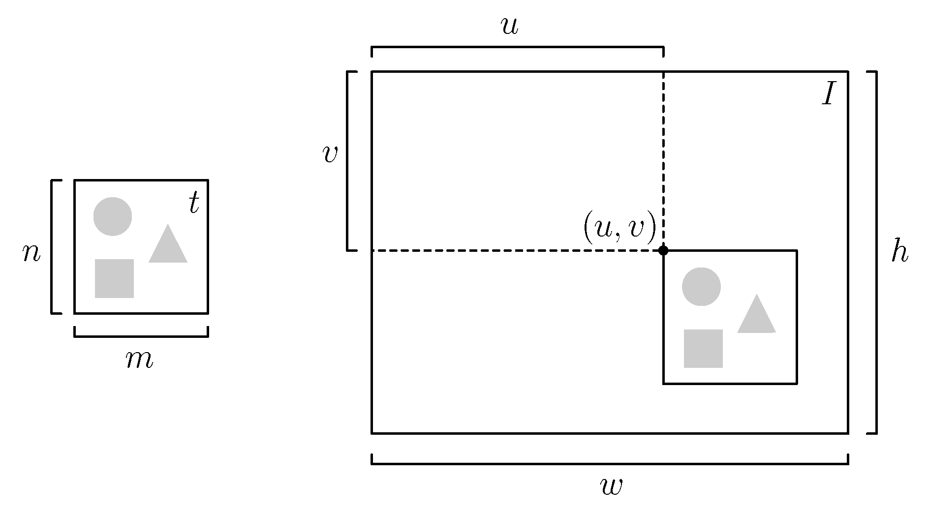
Figure 1. Template t can be contained in frame I in a rectangle of size m × n which has point ( u , v ) as top left corner.
Applsci 10 02122 g001
Figure 2. The original HSA defined a smaller search region around each recruiter. The proposed parallel version defines a unique region that contains the recruiters. (a) Original; (b) New proposal.
Applsci 10 02122 g002
Figure 3. Workflow of programs BEE and NO BEE. The random number generation is only used in program BEE. Parallel NCC is specific to program NO BEE and Parallel HSA is specific to program BEE.
Applsci 10 02122 g003
Figure 4. Example videos from the ALOV dataset (first 7 categories). Only first frames are shown. The target object is enclosed.
Applsci 10 02122 g004
Figure 5. Example videos from the ALOV dataset (last seven categories). Only first frames are shown. The target object is enclosed.
Applsci 10 02122 g005
Figure 6. T i (truth) and G T i (ground truth) may intersect. The PASCAL criterion helps to quantify how similar T i and G T i are, based on this.
Applsci 10 02122 g006
Figure 7. Comparison of F-score between using this work’s NCC (OURS) and another NCC implementation (CTRL), the raw data was obtained from [44]. ’Both’ shows the average and standard deviation of OURS and CTRL combined.
Applsci 10 02122 g007
Figure 8. Comparison of F-score survival curves between using this work’s NCC (OURS) and the NCC implementation reproduced from [3,44] (CTRL). Other video trackers are shown for reference.
Applsci 10 02122 g008
Figure 9. The effects of increasing the number of generations of HSA. (a) Comparison of F-score. (b) Comparison of average time per frame.
Applsci 10 02122 g009
Figure 10. Selecting the optimal number of generations in terms of average time per frame and F-score using the Score-Time Efficiency. (a) Average time per frame vs. F-score vs. generations. (b) Comparison of Score-Time Efficiency.
Applsci 10 02122 g010
Figure 11. Visual example of the results that were obtained using NCC and HSA with two generations. The frames that are shown correspond to the 23th video of the Light category of the ALOV dataset. Every 14th frame is shown.
Applsci 10 02122 g011
Figure 12. (a) Comparison of F-score between using parallel HSA (GPU BEE) or parallel exhaustive search (GPU NO BEE). ’Both’ shows the average and standard deviation of GPU NO BEE and GPU BEE combined. (b) Comparison of F-score survival curves between using parallel HSA (GPU BEE), parallel exhaustive search (NO BEE) or sequential HSA (CPU BEE).
Applsci 10 02122 g012
Figure 13. (a) Comparison of average time per frame between using parallel HSA (GPU BEE) or parallel exhaustive search (GPU NO BEE). ’Both’ shows the average and standard deviation of GPU NO BEE and GPU BEE combined. (b) Comparison of average seconds per frame survival curves between HSA (BEE) and exhaustive search (NO BEE). There are four survival curves, these are also marked as sequential (CPU) or parallel (GPU).
Applsci 10 02122 g013
Figure 14. Comparison of Score-Time Efficiency between using parallel HSA (GPU BEE), parallel exhaustive search (GPU NO BEE) and sequential HSA (CPU BEE).
Applsci 10 02122 g014
Figure 15. Example frames showing visual effect of Gaussian noise as parameters increase. (a) Noise level 0; (b) Noise level 50; (c) Noise level 100.
Applsci 10 02122 g015
Figure 16. (a) Comparison of F-score survival curves between different levels of noise. (b) Comparison of average time per frame survival curves between different levels of noise.
Applsci 10 02122 g016
Figure 17. (a) Comparison of F-score survival curves between GPU BEE (our best tracker proposal), Struck and SiamMask. (b) Comparison of average time per frame survival curves between GPU BEE, CPU NO BEE (conventional NCC), Struck and SiamMask. In the average time per frame axis, the scale from 0.02 to 0.1 is linear but logarithmic above 0.1, in order to contrast substantial difference of average time per frame between CPU NO BEE and the rest of the trackers.
Applsci 10 02122 g017
Table 1. Summary of the configuration parameters used in the tests.
ParameterDescriptionBEENO BEE
μ e Size of all populations64
Generations2
η m Parameter for mutation25
η c Parameter for crossover2
α e / λ e Mutation sons, exploration60%
β e / λ e Crossover sons, exploration10%
γ e / λ e Random sons, exploration30%
α r / λ r Mutation sons, harvest60%
β r / λ r Crossover sons, harvest30%
γ r / λ r Random sons, harvest10%
Table 2. Time Complexity of different implementations to be compared
ImplementationAbbreviationTime Complexity
Sequential exhaustive NCCCPU NO BEE O ( m n w h )
Parallel exhaustive NCCGPU NO BEE O ( m n w h c )
Sequential HSA NCCCPU BEE O ( g λ h m n )
Parallel HSA NCCGPU BEE O ( g m n q )
Table 3. Comparison between using GPU or CPU to compute exhaustive NCC. The average time per frame contemplates all the videos of the dataset, the units are seconds per frame. ’Both’ shows the average and standard deviation of CPU NO BEE and GPU NO BEE combined.
AverageF-Score *F-Score *
Time per FrameAverageDeviation
[spf][arb. unit][arb. unit]
CPU NO BEE202.13990.54530.3056
GPU NO BEE1.18230.50510.3327
Both101.66110.52520.3193
(*) Only 100 random videos of the dataset taken into account.