GIS-Based Gully Erosion Susceptibility Mapping: A Comparison of Computational Ensemble Data Mining Models

 ,
, 
 ,
,  , ,
, ,  ,
, 
 , ,
, , 
Abstract
1. Introduction
2. Materials and Methods
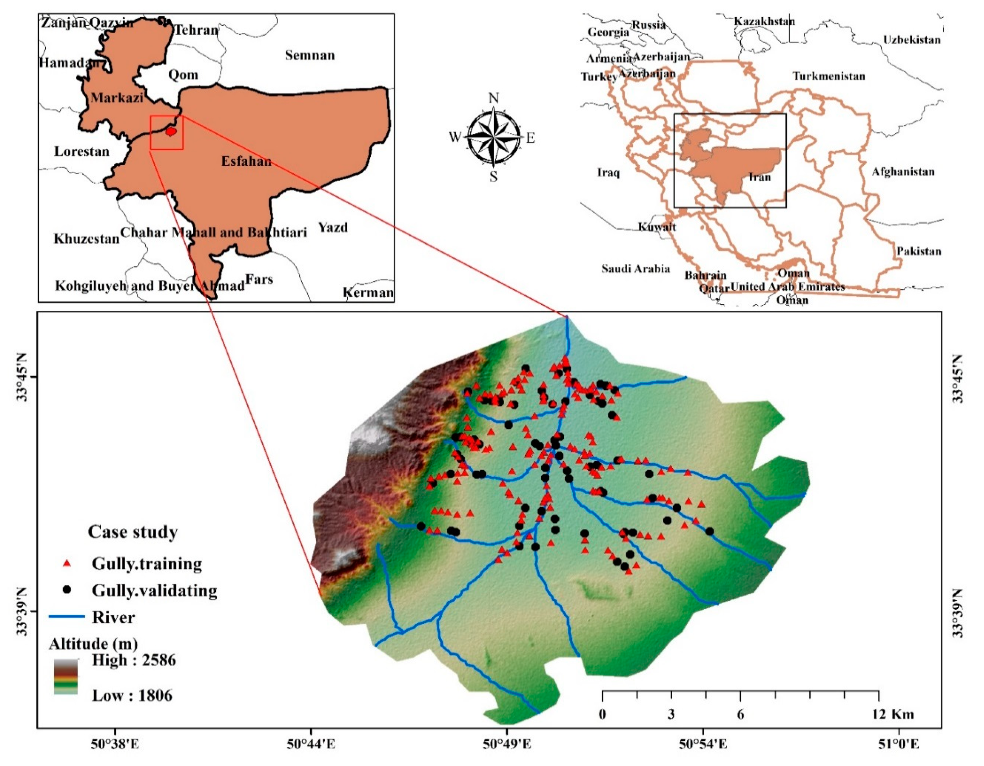
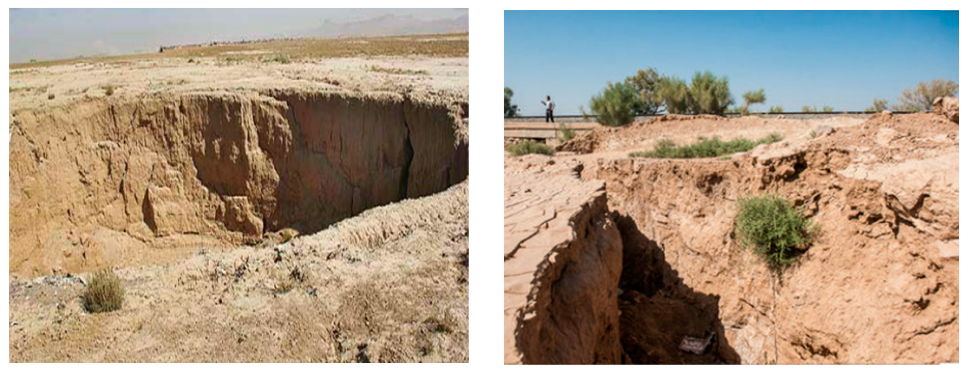
2.1. Study Area
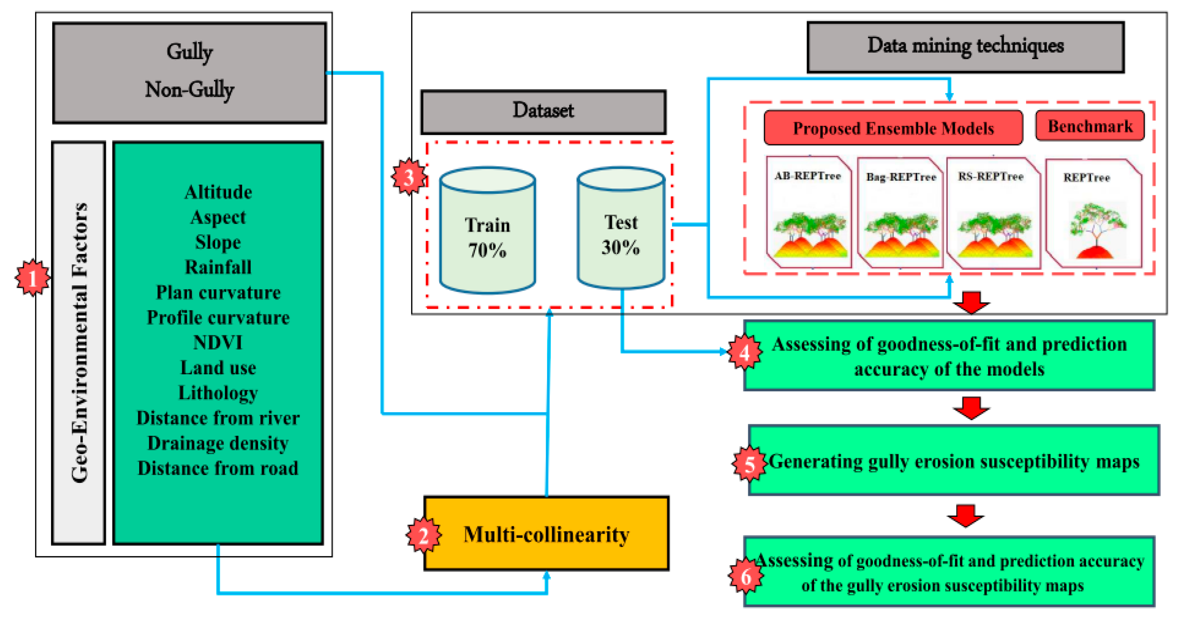
2.2. Methodology
2.2.1. Gully Inventory Map
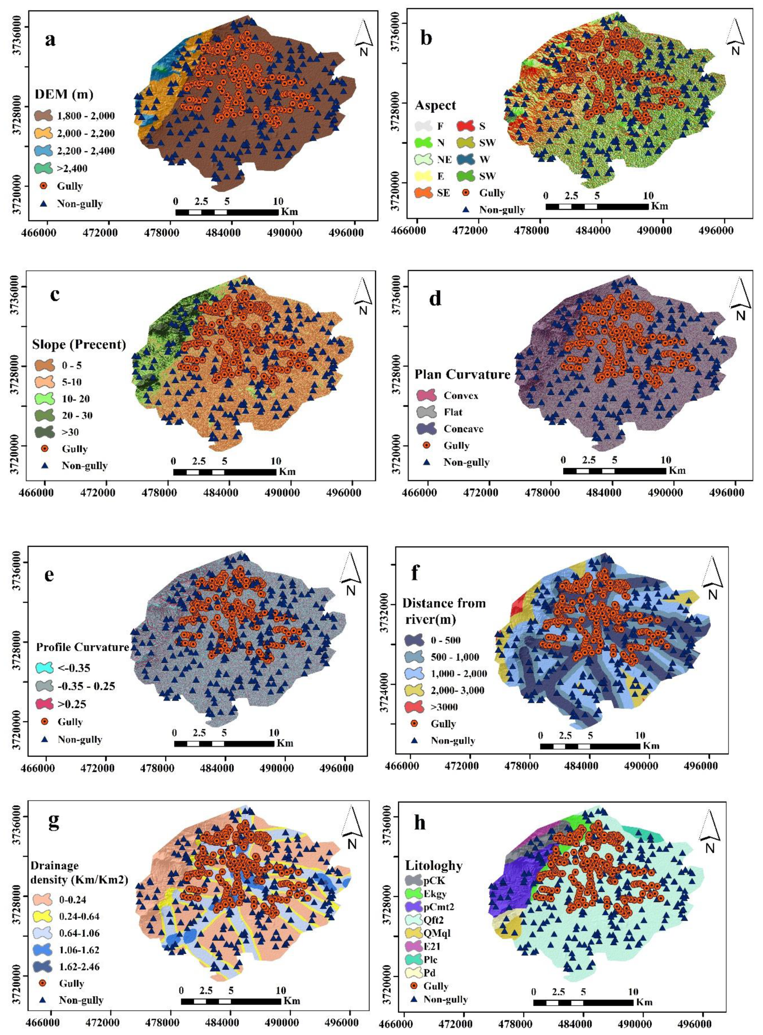
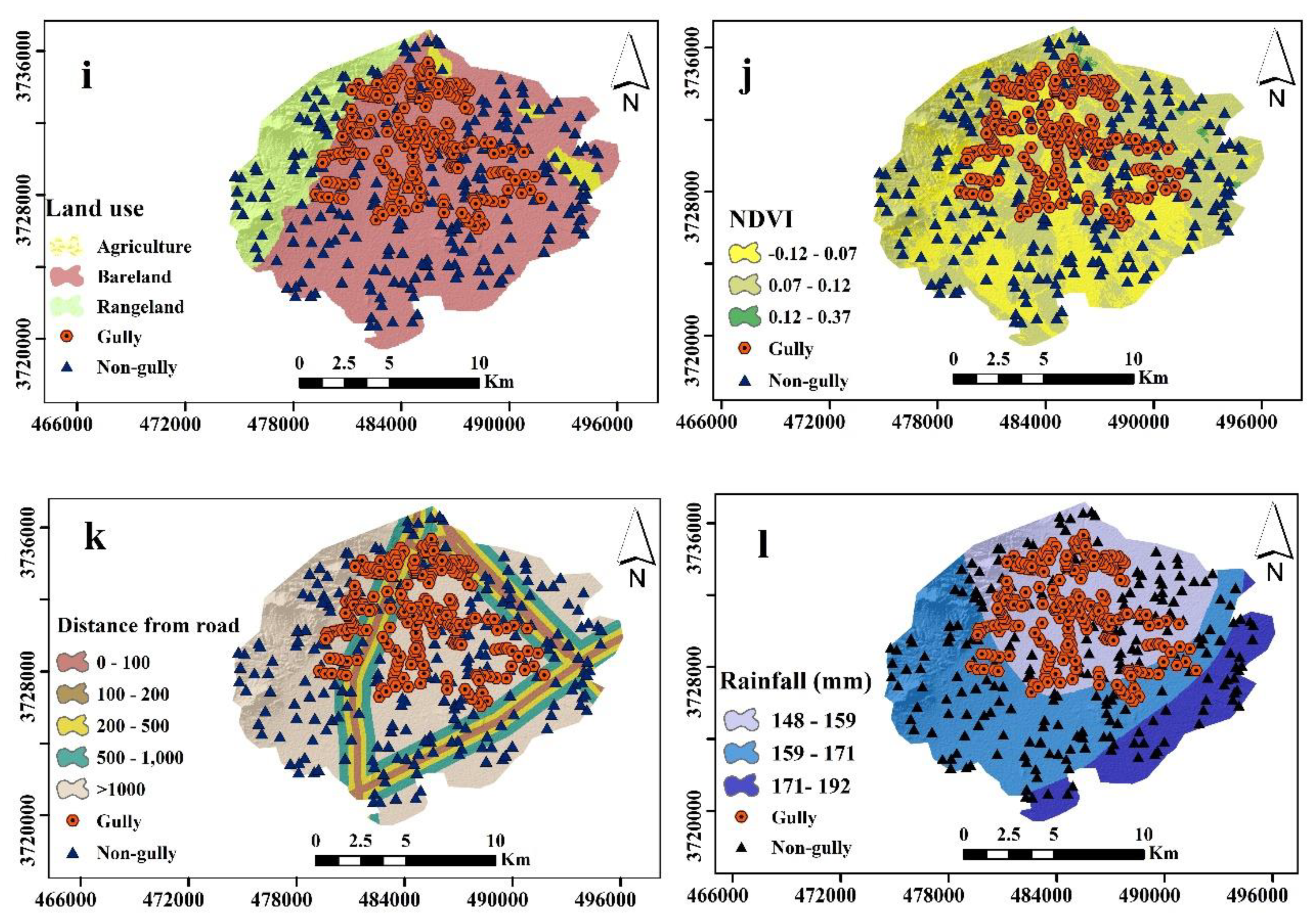
2.2.2. Gully Conditioning Factors
2.2.3. Gully Erosion Susceptibility Modeling
AdaBoost (AB)
Bagging (Bag)
- Input: training set S, inducer T, integer T (number of bootstrap samples)
- (1)
- for i = 1 to T {
- (2)
- = bootstrap sample from S (sample with replacement)
- (3)
- (4)
- }
- (5)
- (6)
- Output: classifier
Random Subspace
- (1)
- Repeat for b = 1, 2, ..., B:
- (a)
- Select a r-dimensional random subspace from the original p-dimensional feature space.
- (b)
- Construct a classifier with a decision boundary in .
- (2)
- Combine classifiers by simple majority voting to obtain a final decision rule:where is the Kronecker symbol and y is a decision (class label) of the classifier.
Reduced-Error Pruning Tree (REPTree)
2.2.4. Comparison and Validation of Gully Erosion Models and Susceptibility Maps
Machine Learning Evaluation Metrics
Error-Based Evaluation Metrics
2.2.5. Factor Ranking and Selection by the Information Gain Ratio Technique
3. Results
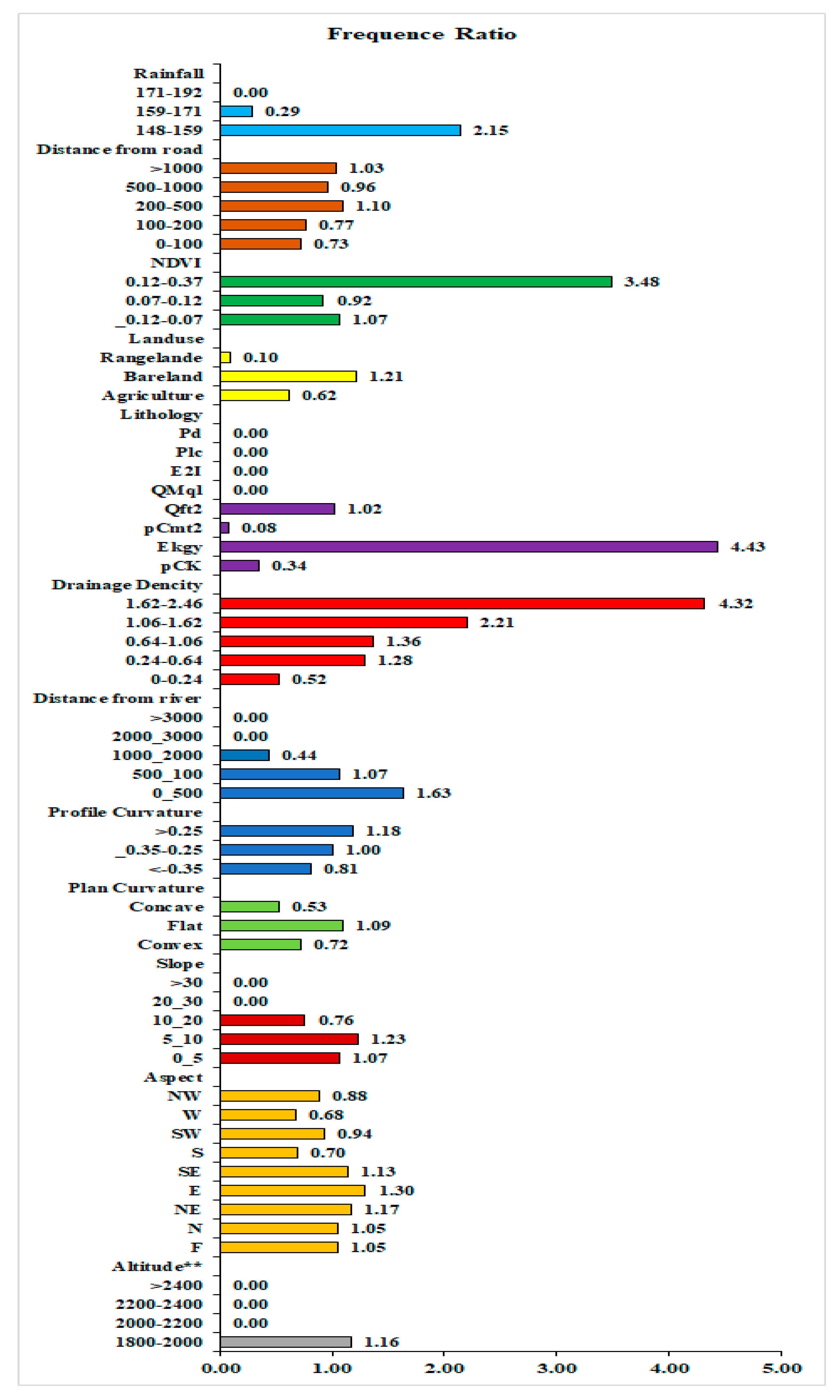
3.1. Correlation between Conditioning Factors and Gully Occurrence Using the Frequency Ratio Method
3.2. Analysis of Factor Multi-Collinearity
3.3. The Most Important Factors for Gully Modeling
3.4. Evaluation of Gully Erosion Susceptibility Models
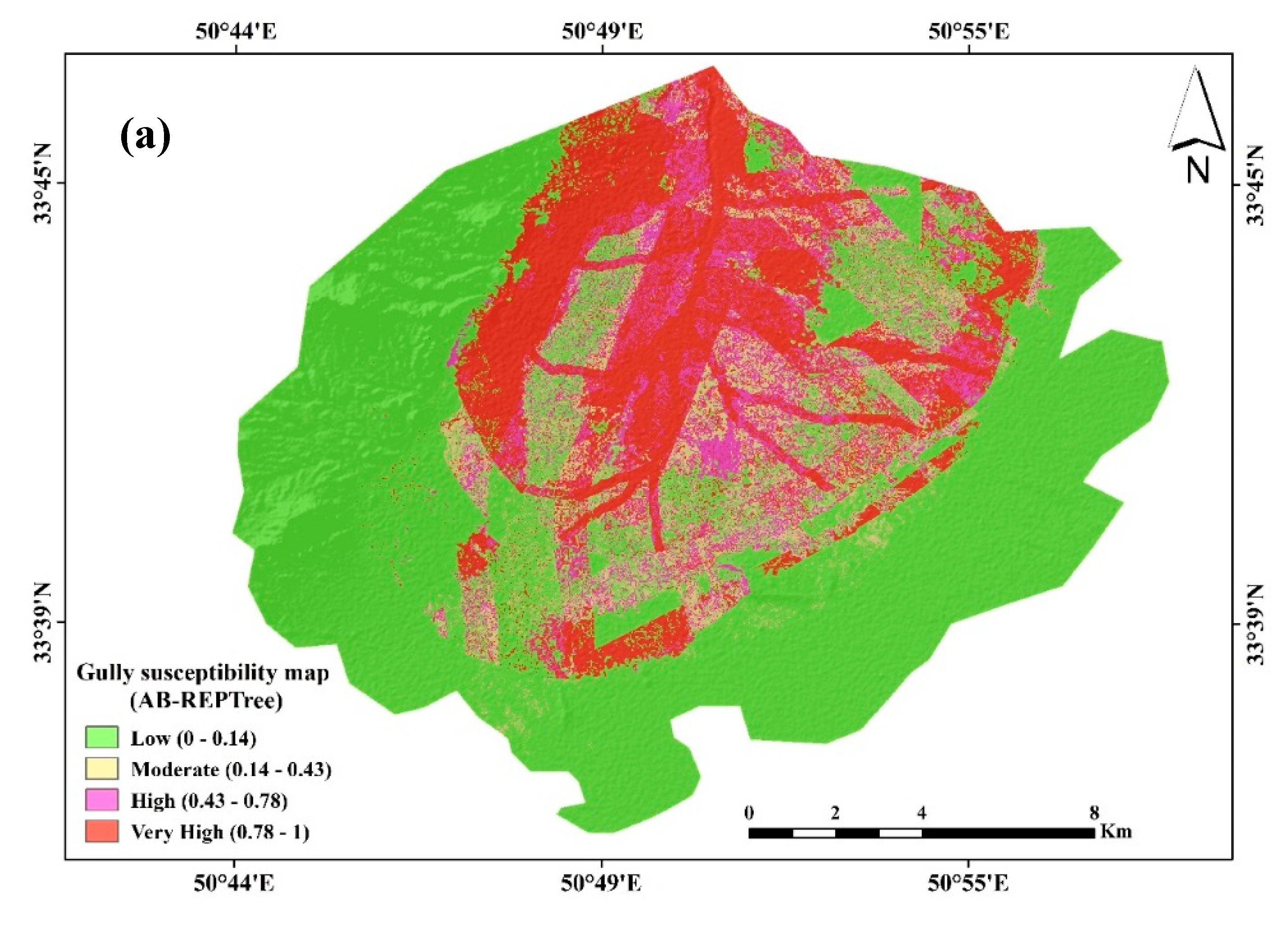
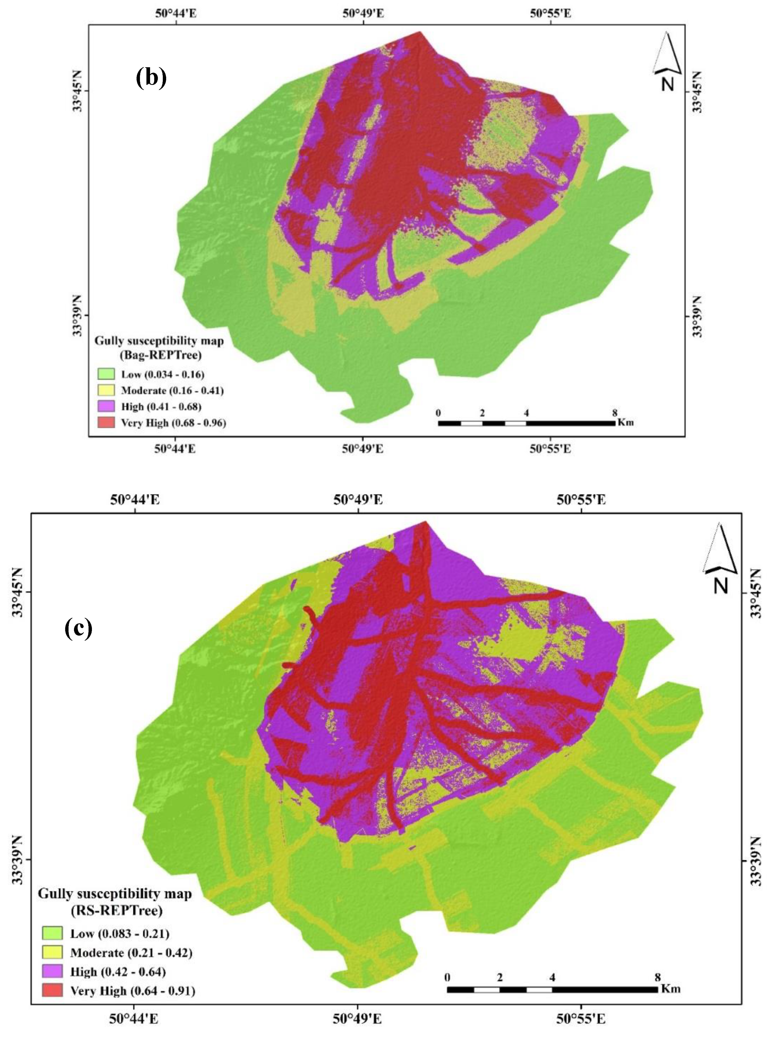
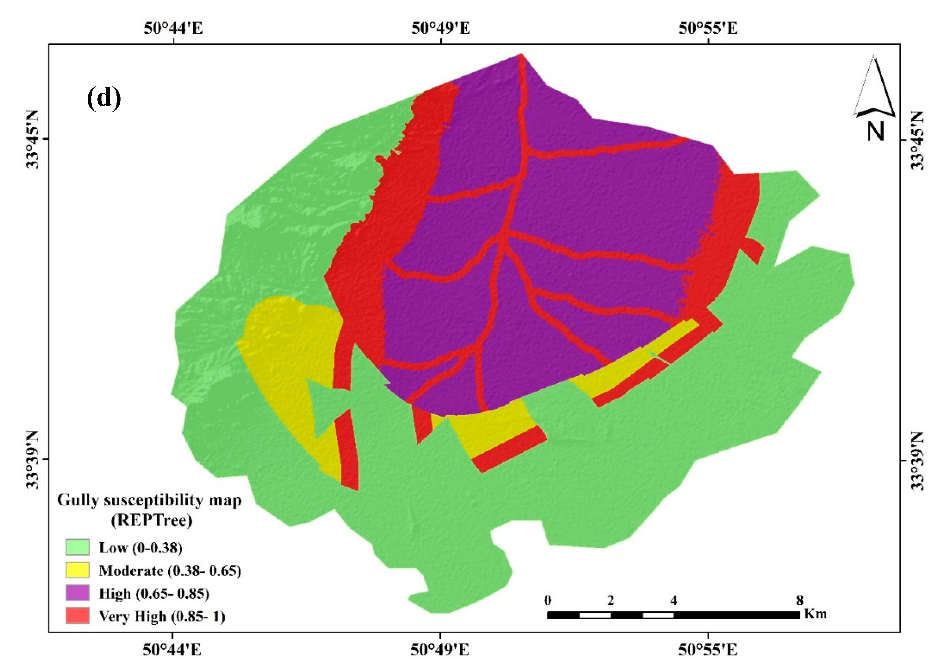
3.5. Development of Gully Erosion Susceptibility Maps
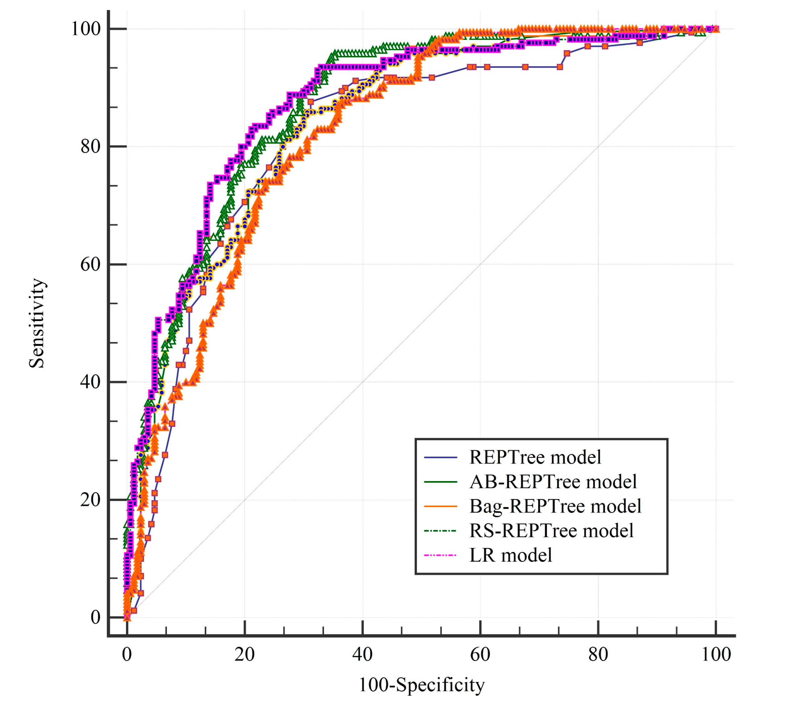
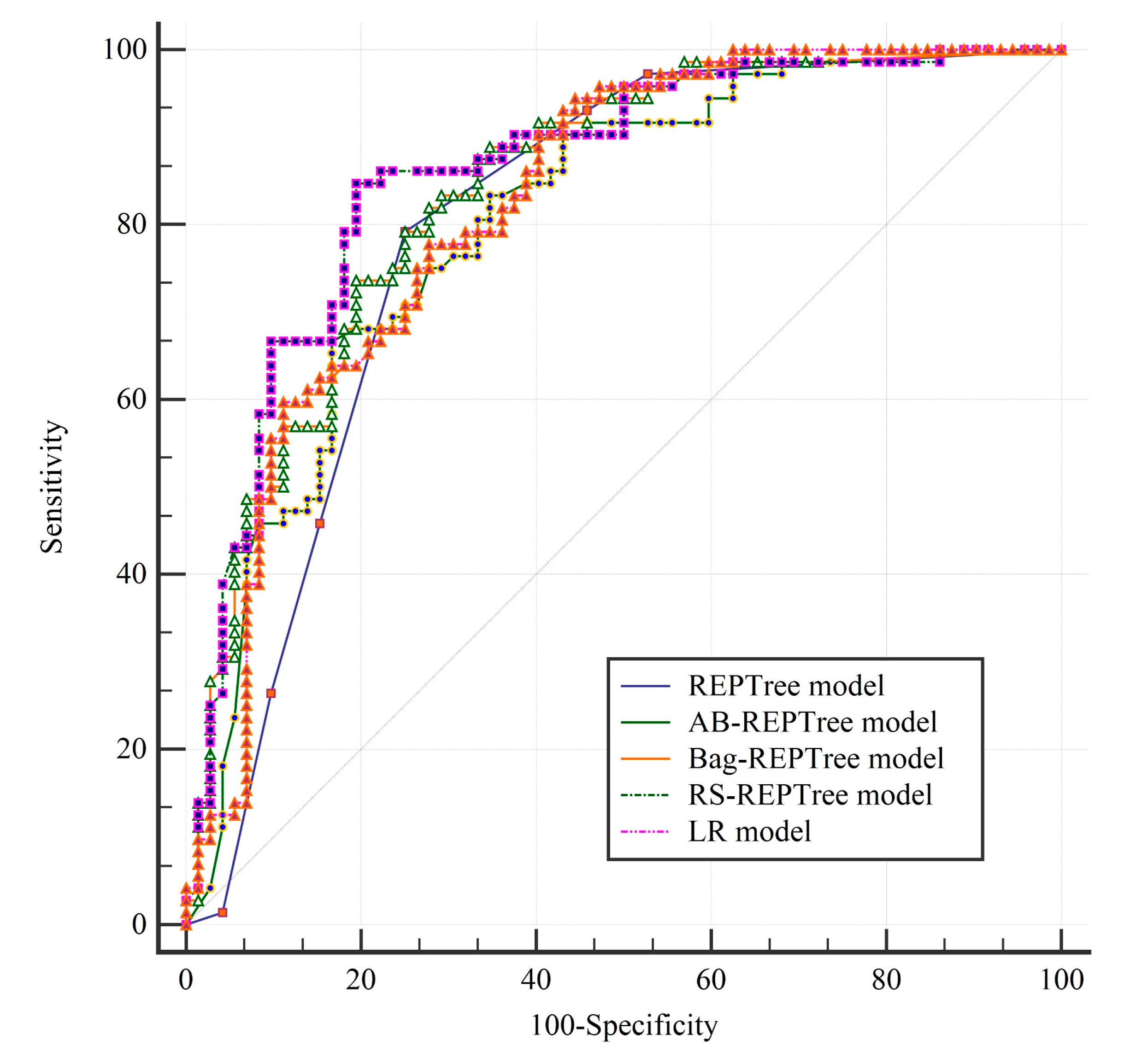
3.6. Evaluation and Comparison of the Models
4. Discussion
5. Conclusions
Author Contributions
Funding
Conflicts of Interest
References
- Morgan, R.P.C. Soil Erosion and Conservation; John Wiley & Sons: Hoboken, NJ, USA, 2009. [Google Scholar]
- Conoscenti, C.; Angileri, S.; Cappadonia, C.; Rotigliano, E.; Agnesi, V.; Märker, M. Gully erosion susceptibility assessment by means of gis-based logistic regression: A case of sicily (Italy). Geomorphology 2014, 204, 399–411. [Google Scholar] [CrossRef]
- Moradi, H.; Avand, M.T.; Janizadeh, S. Landslide susceptibility survey using modeling methods. In Spatial Modeling in Gis and R for Earth and Environmental Sciences; Elsevier: New York, NY, USA, 2019; pp. 259–275. [Google Scholar]
- Ionita, I.; Fullen, M.A.; Zgłobicki, W.; Poesen, J. Gully erosion as a natural and human-induced hazard. Nat. Hazards 2015, 79. [Google Scholar] [CrossRef]
- Ni, H.; Li, Z.; Tie, Y.; Song, Z. Formation condition, disaster characteristics and developing trend analysis on debris flows in moxi river basin, sw China. In Landslide Science for a Safer Geoenvironment; Springer: Berlin/Heidelberg, Germany, 2014; pp. 5–11. [Google Scholar]
- Jurchescu, M.; Grecu, F. Modelling the occurrence of gullies at two spatial scales in the olteţ drainage basin (Romania). Nat. Hazards 2015, 79, 255–289. [Google Scholar] [CrossRef]
- Kirkby, M. Thresholds and Instability in Stream Head Hollows: A Model of Magnitude and Frequency for Wash Processes; School of Geography, University of Leeds: Leeds, UK, 1992. [Google Scholar]
- Lucà, F.; Conforti, M.; Robustelli, G. Comparison of gis-based gullying susceptibility mapping using bivariate and multivariate statistics: Northern Calabria, South Italy. Geomorphology 2011, 134, 297–308. [Google Scholar] [CrossRef]
- Poesen, J.; Vandekerckhove, L.; Nachtergaele, J.; Oostwoud Wijdenes, D.; Verstraeten, G.; van Wesemael, B. Gully erosion in dryland environments. In Dryland Rivers: Hydrology and Geomorphology of Semi-Arid Channels; Bull, L.J., Kirkby, M.J., Eds.; Wiley: Chichester, UK, 2002; pp. 229–262. [Google Scholar]
- Valentin, C.; Poesen, J.; Li, Y. Gully erosion: Impacts, factors and control. Catena 2005, 63, 132–153. [Google Scholar] [CrossRef]
- Istanbulluoglu, E.; Tarboton, D.G.; Pack, R.T.; Luce, C. A probabilistic approach for channel initiation. Water Resour. Res. 2002, 38, 1–14. [Google Scholar] [CrossRef]
- Shellberg, J.; Spencer, J.; Brooks, A.; Pietsch, T. Degradation of the mitchell river fluvial megafan by alluvial gully erosion increased by post-european land use change, queensland, australia. Geomorphology 2016, 266, 105–120. [Google Scholar] [CrossRef]
- Burkard, M.; Kostaschuk, R. Patterns and controls of gully growth along the shoreline of lake huron. Earth Surf. Process. Landf. J. Br. Geomorphol. Group 1997, 22, 901–911. [Google Scholar] [CrossRef]
- Heathwaite, A.L.; Burt, T.; Trudgill, S. Land-use controls on sediment production in a lowland catchment, south-west England. In Soil Erosion on Agricultural Land, Proceedings of the Workshop Sponsored by the British Geomorphological Research Group, Coventry, UK, 17–19 January 1989; John Wiley & Sons Ltd.: Hoboken, NJ, USA, 1990; pp. 69–86. [Google Scholar]
- Nachtergaele, J.; Poesen, J.; Sidorchuk, A.; Torri, D. Prediction of concentrated flow width in ephemeral gully channels. Hydrol. Process. 2002, 16, 1935–1953. [Google Scholar] [CrossRef]
- Nyssen, J.; Poesen, J.; Moeyersons, J.; Luyten, E.; Veyret-Picot, M.; Deckers, J.; Haile, M.; Govers, G. Impact of road building on gully erosion risk: A case study from the northern ethiopian highlands. Earth Surf. Process. Landf. J. Br. Geomorphol. Group 2002, 27, 1267–1283. [Google Scholar] [CrossRef]
- McCloskey, G.; Wasson, R.; Boggs, G.; Douglas, M. Timing and causes of gully erosion in the riparian zone of the semi-arid tropical victoria river, australia: Management implications. Geomorphology 2016, 266, 96–104. [Google Scholar] [CrossRef]
- Wang, Y.; Hong, H.; Chen, W.; Li, S.; Panahi, M.; Khosravi, K.; Shirzadi, A.; Shahabi, H.; Panahi, S.; Costache, R. Flood susceptibility mapping in Dingnan county (China) using adaptive neuro-fuzzy inference system with biogeography based optimization and imperialistic competitive algorithm. J. Environ. Manag. 2019, 247, 712–729. [Google Scholar] [CrossRef] [PubMed]
- Khosravi, K.; Shahabi, H.; Pham, B.T.; Adamowski, J.; Shirzadi, A.; Pradhan, B.; Dou, J.; Ly, H.-B.; Gróf, G.; Ho, H.L. A comparative assessment of flood susceptibility modeling using multi-criteria decision-making analysis and machine learning methods. J. Hydrol. 2019, 573, 311–323. [Google Scholar] [CrossRef]
- He, Q.; Shahabi, H.; Shirzadi, A.; Li, S.; Chen, W.; Wang, N.; Chai, H.; Bian, H.; Ma, J.; Chen, Y. Landslide spatial modelling using novel bivariate statistical based naïve bayes, rbf classifier, and rbf network machine learning algorithms. Sci. Total Environ. 2019, 663, 1–15. [Google Scholar] [CrossRef] [PubMed]
- Tien Bui, D.; Shirzadi, A.; Chapi, K.; Shahabi, H.; Pradhan, B.; Pham, B.T.; Singh, V.P.; Chen, W.; Khosravi, K.; Bin Ahmad, B. A hybrid computational intelligence approach to groundwater spring potential mapping. Water 2019, 11, 2013. [Google Scholar] [CrossRef]
- Tien Bui, D.; Shahabi, H.; Shirzadi, A.; Chapi, K.; Hoang, N.-D.; Pham, B.; Bui, Q.-T.; Tran, C.-T.; Panahi, M.; Bin Ahamd, B. A novel integrated approach of relevance vector machine optimized by imperialist competitive algorithm for spatial modeling of shallow landslides. Remote Sens. 2018, 10, 1538. [Google Scholar] [CrossRef]
- Tien Bui, D.; Khosravi, K.; Li, S.; Shahabi, H.; Panahi, M.; Singh, V.; Chapi, K.; Shirzadi, A.; Panahi, S.; Chen, W. New hybrids of anfis with several optimization algorithms for flood susceptibility modeling. Water 2018, 10, 1210. [Google Scholar] [CrossRef]
- Shafizadeh-Moghadam, H.; Valavi, R.; Shahabi, H.; Chapi, K.; Shirzadi, A. Novel forecasting approaches using combination of machine learning and statistical models for flood susceptibility mapping. J. Environ. Manag. 2018, 217, 1–11. [Google Scholar] [CrossRef]
- Chapi, K.; Singh, V.P.; Shirzadi, A.; Shahabi, H.; Bui, D.T.; Pham, B.T.; Khosravi, K. A novel hybrid artificial intelligence approach for flood susceptibility assessment. Environ. Model. Softw. 2017, 95, 229–245. [Google Scholar] [CrossRef]
- Chen, W.; Li, Y.; Xue, W.; Shahabi, H.; Li, S.; Hong, H.; Wang, X.; Bian, H.; Zhang, S.; Pradhan, B. Modeling flood susceptibility using data-driven approaches of naïve bayes tree, alternating decision tree, and random forest methods. Sci. Total Environ. 2020, 701, 134979. [Google Scholar] [CrossRef]
- Shahabi, H.; Shirzadi, A.; Ghaderi, K.; Omidvar, E.; Al-Ansari, N.; Clague, J.J.; Geertsema, M.; Khosravi, K.; Amini, A.; Bahrami, S. Flood detection and susceptibility mapping using sentinel-1 remote sensing data and a machine learning approach: Hybrid intelligence of bagging ensemble based on k-nearest neighbor classifier. Remote Sens. 2020, 12, 266. [Google Scholar] [CrossRef]
- Khosravi, K.; Melesse, A.M.; Shahabi, H.; Shirzadi, A.; Chapi, K.; Hong, H. Flood susceptibility mapping at Ningdu catchment, China using bivariate and data mining techniques. In Extreme Hydrology and Climate Variability; Elsevier: New York, NY, USA, 2019; pp. 419–434. [Google Scholar]
- Jaafari, A.; Zenner, E.K.; Panahi, M.; Shahabi, H. Hybrid artificial intelligence models based on a neuro-fuzzy system and metaheuristic optimization algorithms for spatial prediction of wildfire probability. Agric. For. Meteorol. 2019, 266, 198–207. [Google Scholar] [CrossRef]
- Taheri, K.; Shahabi, H.; Chapi, K.; Shirzadi, A.; Gutiérrez, F.; Khosravi, K. Sinkhole susceptibility mapping: A comparison between bayes-based machine learning algorithms. Land Degrad. Dev. 2019, 30, 730–745. [Google Scholar] [CrossRef]
- Roodposhti, M.S.; Safarrad, T.; Shahabi, H. Drought sensitivity mapping using two one-class support vector machine algorithms. Atmos. Res. 2017, 193, 73–82. [Google Scholar] [CrossRef]
- Choubin, B.; Soleimani, F.; Pirnia, A.; Sajedi-Hosseini, F.; Alilou, H.; Rahmati, O.; Melesse, A.M.; Singh, V.P.; Shahabi, H. Effects of drought on vegetative cover changes: Investigating spatiotemporal patterns. In Extreme Hydrology and Climate Variability; Elsevier: New York, NY, USA, 2019; pp. 213–222. [Google Scholar]
- Lee, S.; Panahi, M.; Pourghasemi, H.R.; Shahabi, H.; Alizadeh, M.; Shirzadi, A.; Khosravi, K.; Melesse, A.M.; Yekrangnia, M.; Rezaie, F. Sevucas: A novel gis-based machine learning software for seismic vulnerability assessment. Appl. Sci. 2019, 9, 3495. [Google Scholar] [CrossRef]
- Alizadeh, M.; Alizadeh, E.; Asadollahpour Kotenaee, S.; Shahabi, H.; Beiranvand Pour, A.; Panahi, M.; Bin Ahmad, B.; Saro, L. Social vulnerability assessment using Artificial Neural Network (ANN) model for earthquake hazard in Tabriz city, Iran. Sustainability 2018, 10, 3376. [Google Scholar] [CrossRef]
- Tien Bui, D.; Shahabi, H.; Shirzadi, A.; Chapi, K.; Pradhan, B.; Chen, W.; Khosravi, K.; Panahi, M.; Bin Ahmad, B.; Saro, L. Land subsidence susceptibility mapping in south korea using machine learning algorithms. Sensors 2018, 18, 2464. [Google Scholar] [CrossRef]
- Rahmati, O.; Samadi, M.; Shahabi, H.; Azareh, A.; Rafiei-Sardooi, E.; Alilou, H.; Melesse, A.M.; Pradhan, B.; Chapi, K.; Shirzadi, A. Swpt: An automated gis-based tool for prioritization of sub-watersheds based on morphometric and topo-hydrological factors. Geosci. Front. 2019, 10, 2167–2175. [Google Scholar] [CrossRef]
- Choubin, B.; Rahmati, O.; Tahmasebipour, N.; Feizizadeh, B.; Pourghasemi, H.R. Application of fuzzy analytical network process model for analyzing the gully erosion susceptibility. In Natural Hazards GIS-Based Spatial Modeling Using Data Mining Techniques; Springer: Berlin/Heidelberg, Germany, 2019; pp. 105–125. [Google Scholar]
- Chen, W.; Pradhan, B.; Li, S.; Shahabi, H.; Rizeei, H.M.; Hou, E.; Wang, S. Novel hybrid integration approach of bagging-based fisher’s linear discriminant function for groundwater potential analysis. Nat. Resour. Res. 2019, 28, 1239–1258. [Google Scholar] [CrossRef]
- Miraki, S.; Zanganeh, S.H.; Chapi, K.; Singh, V.P.; Shirzadi, A.; Shahabi, H.; Pham, B.T. Mapping groundwater potential using a novel hybrid intelligence approach. Water Resour. Manag. 2019, 33, 281–302. [Google Scholar] [CrossRef]
- Rahmati, O.; Naghibi, S.A.; Shahabi, H.; Bui, D.T.; Pradhan, B.; Azareh, A.; Rafiei-Sardooi, E.; Samani, A.N.; Melesse, A.M. Groundwater spring potential modelling: Comprising the capability and robustness of three different modeling approaches. J. Hydrol. 2018, 565, 248–261. [Google Scholar] [CrossRef]
- Chen, W.; Li, Y.; Tsangaratos, P.; Shahabi, H.; Ilia, I.; Xue, W.; Bian, H. Groundwater spring potential mapping using artificial intelligence approach based on kernel logistic regression, random forest, and alternating decision tree models. Appl. Sci. 2020, 10, 425. [Google Scholar] [CrossRef]
- Avand, M.; Janizadeh, S.; Tien Bui, D.; Pham, V.H.; Ngo, P.T.T.; Nhu, V.H. A tree-based intelligence ensemble approach for spatial prediction of potential groundwater. Int. J. Digit. Earth 2020, 1–22. [Google Scholar] [CrossRef]
- Chen, W.; Tsangaratos, P.; Ilia, I.; Duan, Z.; Chen, X. Groundwater spring potential mapping using population-based evolutionary algorithms and data mining methods. Sci. Total Environ. 2019, 684, 31–49. [Google Scholar] [CrossRef]
- Chen, W.; Zhao, X.; Tsangaratos, P.; Shahabi, H.; Ilia, I.; Xue, W.; Wang, X.; Ahmad, B.B. Evaluating the usage of tree-based ensemble methods in groundwater spring potential mapping. J. Hydrol. 2020, 583, 124602. [Google Scholar] [CrossRef]
- Tien Bui, D.; Shahabi, H.; Shirzadi, A.; Chapi, K.; Alizadeh, M.; Chen, W.; Mohammadi, A.; Ahmad, B.; Panahi, M.; Hong, H. Landslide detection and susceptibility mapping by airsar data using support vector machine and index of entropy models in cameron highlands, malaysia. Remote Sens. 2018, 10, 1527. [Google Scholar] [CrossRef]
- Chen, W.; Peng, J.; Hong, H.; Shahabi, H.; Pradhan, B.; Liu, J.; Zhu, A.-X.; Pei, X.; Duan, Z. Landslide susceptibility modelling using gis-based machine learning techniques for Chongren county, Jiangxi province, China. Sci. Total Environ. 2018, 626, 1121–1135. [Google Scholar] [CrossRef]
- Pham, B.T.; Shirzadi, A.; Shahabi, H.; Omidvar, E.; Singh, S.K.; Sahana, M.; Asl, D.T.; Ahmad, B.B.; Quoc, N.K.; Lee, S. Landslide susceptibility assessment by novel hybrid machine learning algorithms. Sustainability 2019, 11, 4386. [Google Scholar] [CrossRef]
- Shirzadi, A.; Bui, D.T.; Pham, B.T.; Solaimani, K.; Chapi, K.; Kavian, A.; Shahabi, H.; Revhaug, I. Shallow landslide susceptibility assessment using a novel hybrid intelligence approach. Environ. Earth Sci. 2017, 76, 60. [Google Scholar] [CrossRef]
- Pham, B.T.; Prakash, I.; Dou, J.; Singh, S.K.; Trinh, P.T.; Tran, H.T.; Le, T.M.; Van Phong, T.; Khoi, D.K.; Shirzadi, A. A novel hybrid approach of landslide susceptibility modelling using rotation forest ensemble and different base classifiers. Geocarto Int. 2019. [Google Scholar] [CrossRef]
- Pradhan, B. A comparative study on the predictive ability of the decision tree, support vector machine and neuro-fuzzy models in landslide susceptibility mapping using gis. Comput. Geosci. 2013, 51, 350–365. [Google Scholar] [CrossRef]
- Chen, W.; Shahabi, H.; Shirzadi, A.; Hong, H.; Akgun, A.; Tian, Y.; Liu, J.; Zhu, A.-X.; Li, S. Novel hybrid artificial intelligence approach of bivariate statistical-methods-based kernel logistic regression classifier for landslide susceptibility modeling. Bull. Eng. Geol. Environ. 2019, 78, 4397–4419. [Google Scholar] [CrossRef]
- Dou, J.; Yunus, A.P.; Bui, D.T.; Merghadi, A.; Sahana, M.; Zhu, Z.; Chen, C.-W.; Khosravi, K.; Yang, Y.; Pham, B.T. Assessment of advanced random forest and decision tree algorithms for modeling rainfall-induced landslide susceptibility in the Izu-Oshima Volcanic Island, Japan. Sci. Total Environ. 2019, 662, 332–346. [Google Scholar] [CrossRef] [PubMed]
- Jaafari, A.; Panahi, M.; Pham, B.T.; Shahabi, H.; Bui, D.T.; Rezaie, F.; Lee, S. Meta optimization of an adaptive neuro-fuzzy inference system with grey wolf optimizer and biogeography-based optimization algorithms for spatial prediction of landslide susceptibility. Catena 2019, 175, 430–445. [Google Scholar] [CrossRef]
- Hong, H.; Shahabi, H.; Shirzadi, A.; Chen, W.; Chapi, K.; Ahmad, B.B.; Roodposhti, M.S.; Hesar, A.Y.; Tian, Y.; Bui, D.T. Landslide susceptibility assessment at the Wuning area, China: A comparison between multi-criteria decision making, bivariate statistical and machine learning methods. Nat. Hazards 2019, 96, 173–212. [Google Scholar] [CrossRef]
- Shafizadeh-Moghadam, H.; Minaei, M.; Shahabi, H.; Hagenauer, J. Big data in geohazard; pattern mining and large scale analysis of landslides in Iran. Earth Sci. Inform. 2019, 12, 1–17. [Google Scholar] [CrossRef]
- Nguyen, V.V.; Pham, B.T.; Vu, B.T.; Prakash, I.; Jha, S.; Shahabi, H.; Shirzadi, A.; Ba, D.N.; Kumar, R.; Chatterjee, J.M. Hybrid machine learning approaches for landslide susceptibility modeling. Forests 2019, 10, 157. [Google Scholar] [CrossRef]
- Nguyen, P.T.; Tuyen, T.T.; Shirzadi, A.; Pham, B.T.; Shahabi, H.; Omidvar, E.; Amini, A.; Entezami, H.; Prakash, I.; Phong, T.V. Development of a novel hybrid intelligence approach for landslide spatial prediction. Appl. Sci. 2019, 9, 2824. [Google Scholar] [CrossRef]
- Tien Bui, D.; Shahabi, H.; Omidvar, E.; Shirzadi, A.; Geertsema, M.; Clague, J.J.; Khosravi, K.; Pradhan, B.; Pham, B.T.; Chapi, K. Shallow landslide prediction using a novel hybrid functional machine learning algorithm. Remote Sens. 2019, 11, 931. [Google Scholar] [CrossRef]
- Tien Bui, D.; Shirzadi, A.; Shahabi, H.; Geertsema, M.; Omidvar, E.; Clague, J.J.; Thai Pham, B.; Dou, J.; Talebpour Asl, D.; Bin Ahmad, B. New ensemble models for shallow landslide susceptibility modeling in a semi-arid watershed. Forests 2019, 10, 743. [Google Scholar] [CrossRef]
- Chen, W.; Zhao, X.; Shahabi, H.; Shirzadi, A.; Khosravi, K.; Chai, H.; Zhang, S.; Zhang, L.; Ma, J.; Chen, Y. Spatial prediction of landslide susceptibility by combining evidential belief function, logistic regression and logistic model tree. Geocarto Int. 2019, 34, 1177–1201. [Google Scholar] [CrossRef]
- Shirzadi, A.; Solaimani, K.; Roshan, M.H.; Kavian, A.; Chapi, K.; Shahabi, H.; Keesstra, S.; Ahmad, B.B.; Bui, D.T. Uncertainties of prediction accuracy in shallow landslide modeling: Sample size and raster resolution. Catena 2019, 178, 172–188. [Google Scholar] [CrossRef]
- Shirzadi, A.; Soliamani, K.; Habibnejhad, M.; Kavian, A.; Chapi, K.; Shahabi, H.; Chen, W.; Khosravi, K.; Thai Pham, B.; Pradhan, B. Novel gis based machine learning algorithms for shallow landslide susceptibility mapping. Sensors 2018, 18, 3777. [Google Scholar] [CrossRef] [PubMed]
- Chen, W.; Shahabi, H.; Zhang, S.; Khosravi, K.; Shirzadi, A.; Chapi, K.; Pham, B.; Zhang, T.; Zhang, L.; Chai, H. Landslide susceptibility modeling based on gis and novel bagging-based kernel logistic regression. Appl. Sci. 2018, 8, 2540. [Google Scholar] [CrossRef]
- Zhang, T.; Han, L.; Chen, W.; Shahabi, H. Hybrid integration approach of entropy with logistic regression and support vector machine for landslide susceptibility modeling. Entropy 2018, 20, 884. [Google Scholar] [CrossRef]
- Abedini, M.; Ghasemian, B.; Shirzadi, A.; Shahabi, H.; Chapi, K.; Pham, B.T.; Bin Ahmad, B.; Tien Bui, D. A novel hybrid approach of bayesian logistic regression and its ensembles for landslide susceptibility assessment. Geocarto Int. 2019, 34, 1427–1457. [Google Scholar] [CrossRef]
- Chen, W.; Xie, X.; Peng, J.; Shahabi, H.; Hong, H.; Bui, D.T.; Duan, Z.; Li, S.; Zhu, A.-X. Gis-based landslide susceptibility evaluation using a novel hybrid integration approach of bivariate statistical based random forest method. Catena 2018, 164, 135–149. [Google Scholar] [CrossRef]
- Chen, W.; Shirzadi, A.; Shahabi, H.; Ahmad, B.B.; Zhang, S.; Hong, H.; Zhang, N. A novel hybrid artificial intelligence approach based on the rotation forest ensemble and naïve bayes tree classifiers for a landslide susceptibility assessment in Langao county, China. Geomat. Nat. Hazards Risk 2017, 8, 1955–1977. [Google Scholar] [CrossRef]
- Hong, H.; Liu, J.; Zhu, A.-X.; Shahabi, H.; Pham, B.T.; Chen, W.; Pradhan, B.; Bui, D.T. A novel hybrid integration model using support vector machines and random subspace for weather-triggered landslide susceptibility assessment in the Wuning area (China). Environ. Earth Sci. 2017, 76, 652. [Google Scholar] [CrossRef]
- Shadman Roodposhti, M.; Aryal, J.; Shahabi, H.; Safarrad, T. Fuzzy shannon entropy: A hybrid gis-based landslide susceptibility mapping method. Entropy 2016, 18, 343. [Google Scholar] [CrossRef]
- Shahabi, H.; Hashim, M.; Ahmad, B.B. Remote sensing and gis-based landslide susceptibility mapping using frequency ratio, logistic regression, and fuzzy logic methods at the central zab basin, Iran. Environ. Earth Sci. 2015, 73, 8647–8668. [Google Scholar] [CrossRef]
- Shahabi, H.; Khezri, S.; Ahmad, B.B.; Hashim, M. Landslide susceptibility mapping at central zab basin, Iran: A comparison between analytical hierarchy process, frequency ratio and logistic regression models. Catena 2014, 115, 55–70. [Google Scholar] [CrossRef]
- Zhao, X.; Chen, W. Gis-based evaluation of landslide susceptibility models using certainty factors and functional trees-based ensemble techniques. Appl. Sci. 2020, 10, 16. [Google Scholar] [CrossRef]
- Abedini, M.; Ghasemian, B.; Shirzadi, A.; Bui, D.T. A comparative study of support vector machine and logistic model tree classifiers for shallow landslide susceptibility modeling. Environ. Earth Sci. 2019, 78, 560. [Google Scholar] [CrossRef]
- Chaplot, V.; Le Brozec, E.C.; Silvera, N.; Valentin, C. Spatial and temporal assessment of linear erosion in catchments under sloping lands of northern laos. Catena 2005, 63, 167–184. [Google Scholar] [CrossRef]
- Kornejady, A.; Ownegh, M.; Bahremand, A. Landslide susceptibility assessment using maximum entropy model with two different data sampling methods. Catena 2017, 152, 144–162. [Google Scholar] [CrossRef]
- Tien Bui, D.; Shirzadi, A.; Shahabi, H.; Chapi, K.; Omidavr, E.; Pham, B.T.; Talebpour Asl, D.; Khaledian, H.; Pradhan, B.; Panahi, M. A novel ensemble artificial intelligence approach for gully erosion mapping in a semi-arid watershed (Iran). Sensors 2019, 19, 2444. [Google Scholar] [CrossRef]
- Pham, B.T.; Avand, M.; Janizadeh, S.; Phong, T.V.; Al-Ansari, N.; Ho, L.S.; Jafari, F. GIS Based Hybrid Computational Approaches for Flash Flood Susceptibility Assessment. Water 2020, 12, 683. [Google Scholar] [CrossRef]
- Pourghasemi, H.R.; Yousefi, S.; Kornejady, A.; Cerdà, A. Performance assessment of individual and ensemble data-mining techniques for gully erosion modeling. Sci. Total Environ. 2017, 609, 764–775. [Google Scholar] [CrossRef]
- Yariyan, P.; Avand, M.; Soltani, F.; Ghorbanzadeh, O.; Blaschke, T. Earthquake Vulnerability Mapping Using Different Hybrid Models. Symmetry 2020, 12, 405. [Google Scholar] [CrossRef]
- Nguyen, M.D.; Pham, B.T.; Tuyen, T.T.; Yen, H.; Phan, H.; Prakash, I.; Vu, T.T.; Chapi, K.; Shirzadi, A.; Shahabi, H. Development of an artificial intelligence approach for prediction of consolidation coefficient of soft soil: A sensitivity analysis. Open Constr. Build. Technol. J. 2019, 13. [Google Scholar] [CrossRef]
- Hosseinalizadeh, M.; Kariminejad, N.; Chen, W.; Pourghasemi, H.R.; Alinejad, M.; Behbahani, A.M.; Tiefenbacher, J.P. Spatial modelling of gully headcuts using uav data and four best-first decision classifier ensembles (bftree, bag-bftree, rs-bftree, and rf-bftree). Geomorphology 2019, 329, 184–193. [Google Scholar] [CrossRef]
- Azareh, A.; Rahmati, O.; Rafiei-Sardooi, E.; Sankey, J.B.; Lee, S.; Shahabi, H.; Ahmad, B.B. Modelling gully-erosion susceptibility in a semi-arid region, Iran: Investigation of applicability of certainty factor and maximum entropy models. Sci. Total Environ. 2019, 655, 684–696. [Google Scholar] [CrossRef] [PubMed]
- Shahabi, H.; Jarihani, B.; Tavakkoli Piralilou, S.; Chittleborough, D.; Avand, M.; Ghorbanzadeh, O. A Semi-Automated Object-Based Gully Networks Detection Using Different Machine Learning Models: A Case Study of Bowen Catchment, Queensland, Australia. Sensors 2019, 19, 4893. [Google Scholar] [CrossRef]
- Ahmadlou, M.; Karimi, M.; Alizadeh, S.; Shirzadi, A.; Parvinnejhad, D.; Shahabi, H.; Panahi, M. Flood susceptibility assessment using integration of Adaptive Network-Based Fuzzy Inference System (ANFIS) and Biogeography-Based Optimization (BBO) and Bat Algorithms (BA). Geocarto Int. 2019, 34, 1252–1272. [Google Scholar] [CrossRef]
- Bui, D.T.; Panahi, M.; Shahabi, H.; Singh, V.P.; Shirzadi, A.; Chapi, K.; Khosravi, K.; Chen, W.; Panahi, S.; Li, S. Novel hybrid evolutionary algorithms for spatial prediction of floods. Sci. Rep. 2018, 8, 1–14. [Google Scholar] [CrossRef]
- Chen, W.; Hong, H.; Panahi, M.; Shahabi, H.; Wang, Y.; Shirzadi, A.; Pirasteh, S.; Alesheikh, A.A.; Khosravi, K.; Panahi, S. Spatial prediction of landslide susceptibility using gis-based data mining techniques of anfis with Whale Optimization Algorithm (WOA) and Grey Wolf Optimizer (GWO). Appl. Sci. 2019, 9, 3755. [Google Scholar] [CrossRef]
- Shirzadi, A.; Shahabi, H.; Chapi, K.; Bui, D.T.; Pham, B.T.; Shahedi, K.; Ahmad, B.B. A comparative study between popular statistical and machine learning methods for simulating volume of landslides. Catena 2017, 157, 213–226. [Google Scholar] [CrossRef]
- Khosravi, K.; Pham, B.T.; Chapi, K.; Shirzadi, A.; Shahabi, H.; Revhaug, I.; Prakash, I.; Bui, D.T. A comparative assessment of decision trees algorithms for flash flood susceptibility modeling at haraz watershed, Northern Iran. Sci. Total Environ. 2018, 627, 744–755. [Google Scholar] [CrossRef]
- Chen, W.; Shahabi, H.; Shirzadi, A.; Li, T.; Guo, C.; Hong, H.; Li, W.; Pan, D.; Hui, J.; Ma, M. A novel ensemble approach of bivariate statistical-based logistic model tree classifier for landslide susceptibility assessment. Geocarto Int. 2018, 33, 1398–1420. [Google Scholar] [CrossRef]
- Gómez-Gutiérrez, Á.; Conoscenti, C.; Angileri, S.E.; Rotigliano, E.; Schnabel, S. Using topographical attributes to evaluate gully erosion proneness (susceptibility) in two mediterranean basins: Advantages and limitations. Nat. Hazards 2015, 79, 291–314. [Google Scholar] [CrossRef]
- Gayen, A.; Pourghasemi, H.R. Spatial modeling of gully erosion: A new ensemble of cart and glm data-mining algorithms. In Spatial Modeling in Gis and R for Earth and Environmental Sciences; Elsevier: New York, NY, USA, 2019; pp. 653–669. [Google Scholar]
- Garosi, Y.; Sheklabadi, M.; Conoscenti, C.; Pourghasemi, H.R.; Van Oost, K. Assessing the performance of gis-based machine learning models with different accuracy measures for determining susceptibility to gully erosion. Sci. Total Environ. 2019, 664, 1117–1132. [Google Scholar] [CrossRef] [PubMed]
- Avand, M.; Janizadeh, S.; Naghibi, S.A.; Pourghasemi, H.R.; Khosrobeigi Bozchaloei, S.; Blaschke, T. A comparative assessment of random forest and k-nearest neighbor classifiers for gully erosion susceptibility mapping. Water 2019, 11, 2076. [Google Scholar] [CrossRef]
- Pham, B.T.; Prakash, I.; Singh, S.K.; Shirzadi, A.; Shahabi, H.; Bui, D.T. Landslide susceptibility modeling using reduced error pruning trees and different ensemble techniques: Hybrid machine learning approaches. Catena 2019, 175, 203–218. [Google Scholar] [CrossRef]
- Pham, B.T.; Jaafari, A.; Prakash, I.; Singh, S.K.; Quoc, N.K.; Bui, D.T. Hybrid computational intelligence models for groundwater potential mapping. Catena 2019, 182, 104101. [Google Scholar] [CrossRef]
- Dube, F.; Nhapi, I.; Murwira, A.; Gumindoga, W.; Goldin, J.; Mashauri, D. Potential of weight of evidence modelling for gully erosion hazard assessment in mbire district–zimbabwe. Phys. Chem. Earth Parts A/B/C 2014, 67, 145–152. [Google Scholar] [CrossRef]
- Rahmati, O.; Pourghasemi, H.R.; Zeinivand, H. Flood susceptibility mapping using frequency ratio and weights-of-evidence models in the Golastan province, Iran. Geocarto Int. 2016, 31, 42–70. [Google Scholar] [CrossRef]
- Janizadeh, S.; Avand, M.; Jaafari, A.; Phong, T.V.; Bayat, M.; Ahmadisharaf, E.; Prakash, I.; Pham, B.T.; Lee, S. Prediction success of machine learning methods for flash flood susceptibility mapping in the tafresh watershed, Iran. Sustainability 2019, 11, 5426. [Google Scholar] [CrossRef]
- Rengers, F.K.; Tucker, G. Analysis and modeling of gully headcut dynamics, north american high plains. J. Geophys. Res. Earth Surf. 2014, 119, 983–1003. [Google Scholar] [CrossRef]
- Hosseinalizadeh, M.; Kariminejad, N.; Chen, W.; Pourghasemi, H.R.; Alinejad, M.; Behbahani, A.M.; Tiefenbacher, J.P. Gully headcut susceptibility modeling using functional trees, naïve bayes tree, and random forest models. Geoderma 2019, 342, 1–11. [Google Scholar] [CrossRef]
- Oostwoud Wijdenes, D.; BRYAN, R. The significance of gully headcuts as a source of sediment on low-angle slopes at baringo, kenya, and initial control measures. Adv. Geoecol. 1994, 27, 205–231. [Google Scholar]
- Wijdenes, D.J.O.; Poesen, J.; Vandekerckhove, L.; Ghesquiere, M. Spatial distribution of gully head activity and sediment supply along an ephemeral channel in a mediterranean environment. Catena 2000, 39, 147–167. [Google Scholar] [CrossRef]
- Kuhnert, P.M.; Henderson, A.K.; Bartley, R.; Herr, A. Incorporating uncertainty in gully erosion calculations using the random forests modelling approach. Environmetrics 2010, 21, 493–509. [Google Scholar] [CrossRef]
- Garosi, Y.; Sheklabadi, M.; Pourghasemi, H.R.; Besalatpour, A.A.; Conoscenti, C.; Van Oost, K. Comparison of differences in resolution and sources of controlling factors for gully erosion susceptibility mapping. Geoderma 2018, 330, 65–78. [Google Scholar] [CrossRef]
- Rahmati, O.; Haghizadeh, A.; Pourghasemi, H.R.; Noormohamadi, F. Gully erosion susceptibility mapping: The role of gis-based bivariate statistical models and their comparison. Nat. Hazards 2016, 82, 1231–1258. [Google Scholar] [CrossRef]
- Di Stefano, C.; Ferro, V.; Palmeri, V.; Pampalone, V. Testing slope effect on flow resistance equation for mobile bed rills. Hydrol. Process. 2018, 32, 664–671. [Google Scholar] [CrossRef]
- Kariminejad, N.; Hosseinalizadeh, M.; Pourghasemi, H.R.; Bernatek-Jakiel, A.; Campetella, G.; Ownegh, M. Evaluation of factors affecting gully headcut location using summary statistics and the maximum entropy model: Golestan province, ne Iran. Sci. Total Environ. 2019, 677, 281–298. [Google Scholar] [CrossRef]
- Zakerinejad, R.; Maerker, M. An integrated assessment of soil erosion dynamics with special emphasis on gully erosion in the mazayjan basin, southwestern Iran. Nat. Hazards 2015, 79, 25–50. [Google Scholar] [CrossRef]
- Frankl, A.; Poesen, J.; Deckers, J.; Haile, M.; Nyssen, J. Gully head retreat rates in the semi-arid highlands of northern ethiopia. Geomorphology 2012, 173, 185–195. [Google Scholar] [CrossRef]
- Svoray, T.; Markovitch, H. Catchment scale analysis of the effect of topography, tillage direction and unpaved roads on ephemeral gully incision. Earth Surf. Process. Landf. J. Br. Geomorphol. Res. Group 2009, 34, 1970–1984. [Google Scholar] [CrossRef]
- Freund, Y.; Schapire, R.E. Experiments with a new boosting algorithm. In Proceedings of the 13th International Conference on Machine Learning, Bari, Italy, 3–6 July 1996; Citeseer: Gaithersburg, MD, USA, 1996; pp. 148–156. [Google Scholar]
- Breiman, L. Bagging predictors. Mach. Learn. 1996, 24, 123–140. [Google Scholar] [CrossRef]
- Efron, B.; Tibshirani, R.J. An Introduction to the Bootstrap; CRC Press: Boca Raton, FL, USA, 1994. [Google Scholar]
- Quinlan, J.R. Simplifying decision trees. Int. J. Man-Mach. Stud. 1987, 27, 221–234. [Google Scholar] [CrossRef]
- Matthews, B.W. Comparison of the predicted and observed secondary structure of t4 phage lysozyme. Biochim. Biophys. Acta (BBA)-Protein Struct. 1975, 405, 442–451. [Google Scholar] [CrossRef]
- Fawcett, T. An introduction to roc analysis. Pattern Recognit. Lett. 2006, 27, 861–874. [Google Scholar] [CrossRef]
- Pham, B.T.; Bui, D.T.; Dholakia, M.; Prakash, I.; Pham, H.V. A comparative study of least square support vector machines and multiclass alternating decision trees for spatial prediction of rainfall-induced landslides in a tropical cyclones area. Geotech. Geol. Eng. 2016, 34, 1807–1824. [Google Scholar] [CrossRef]
- Saito, T.; Rehmsmeier, M. The precision-recall plot is more informative than the roc plot when evaluating binary classifiers on imbalanced datasets. PLoS ONE 2015, 10, e0118432. [Google Scholar] [CrossRef] [PubMed]
- Duch, W.; Winiarski, T.; Biesiada, J.; Kachel, A. Feature selection and ranking filters. In Proceedings of the International Conference on Artificial Neural Networks (ICANN) and International Conference on Neural Information Processing (ICONIP), Istanbul, Turkey, 26–29 June 2003; p. 254. [Google Scholar]
- Nandhini, M.; Sivanandam, S. An improved predictive association rule based classifier using gain ratio and t-test for health care data diagnosis. Sadhana 2015, 40, 1683–1699. [Google Scholar] [CrossRef]
- Amiri, M.; Pourghasemi, H.R.; Ghanbarian, G.A.; Afzali, S.F. Assessment of the importance of gully erosion effective factors using boruta algorithm and its spatial modeling and mapping using three machine learning algorithms. Geoderma 2019, 340, 55–69. [Google Scholar] [CrossRef]
- Rahmati, O.; Tahmasebipour, N.; Haghizadeh, A.; Pourghasemi, H.R.; Feizizadeh, B. Evaluation of different machine learning models for predicting and mapping the susceptibility of gully erosion. Geomorphology 2017, 298, 118–137. [Google Scholar] [CrossRef]
- Pham, B.T.; Prakash, I.; Bui, D.T. Spatial prediction of landslides using a hybrid machine learning approach based on random subspace and classification and regression trees. Geomorphology 2018, 303, 256–270. [Google Scholar] [CrossRef]
- Hong, H.; Liu, J.; Bui, D.T.; Pradhan, B.; Acharya, T.D.; Pham, B.T.; Zhu, A.-X.; Chen, W.; Ahmad, B.B. Landslide susceptibility mapping using j48 decision tree with adaboost, bagging and rotation forest ensembles in the guangchang area (China). Catena 2018, 163, 399–413. [Google Scholar] [CrossRef]
- Arabameri, A.; Chen, W.; Lombardo, L.; Blaschke, T.; Tien Bui, D. Hybrid computational intelligence models for improvement gully erosion assessment. Remote Sens. 2020, 12, 140. [Google Scholar] [CrossRef]
- Gayen, A.; Pourghasemi, H.R.; Saha, S.; Keesstra, S.; Bai, S. Gully erosion susceptibility assessment and management of hazard-prone areas in india using different machine learning algorithms. Sci. Total Environ. 2019, 668, 124–138. [Google Scholar] [CrossRef]
- Vandekerckhove, L.; Poesen, J.; Oostwoud Wijdenes, D.; Nachtergaele, J.; Kosmas, C.; Roxo, M.; De Figueiredo, T. Thresholds for gully initiation and sedimentation in mediterranean europe. Earth Surf. Process. Landf. 2000, 25, 1201–1220. [Google Scholar] [CrossRef]
- Bergonse, R.; Reis, E. Controlling factors of the size and location of large gully systems: A regression-based exploration using reconstructed pre-erosion topography. Catena 2016, 147, 621–631. [Google Scholar] [CrossRef]
- Bayat, M.; Ghorbanpour, M.; Zare, R.; Jaafari, A.; Pham, B.T. Application of artificial neural networks for predicting tree survival and mortality in the hyrcanian forest of Iran. Comput. Electron. Agric. 2019, 164, 104929. [Google Scholar] [CrossRef]
- Van Dao, D.; Jaafari, A.; Bayat, M.; Mafi-Gholami, D.; Qi, C.; Moayedi, H.; Van Phong, T.; Ly, H.-B.; Le, T.-T.; Trinh, P.T. A spatially explicit deep learning neural network model for the prediction of landslide susceptibility. Catena 2020, 188, 104451. [Google Scholar]
- Qiao, W.; Huang, K.; Azimi, M.; Han, S. A novel hybrid prediction model for hourly gas consumption in supply side based on improved whale optimization algorithm and relevance vector machine. IEEE Access 2019, 7, 88218–88230. [Google Scholar] [CrossRef]
- Zhou, G.; Moayedi, H.; Bahiraei, M.; Lyu, Z. Employing artificial bee colony and particle swarm techniques for optimizing a neural network in prediction of heating and cooling loads of residential buildings. J. Clean. Prod. 2020, 120082. [Google Scholar] [CrossRef]
- Ujoh, F.; Igbawua, T.; Ogidi Paul, M. Suitability mapping for rice cultivation in Benue State, Nigeria using satellite data. Geo. Spatial. Inform. Sci 2019, 22, 332–344. [Google Scholar] [CrossRef]


| Predicted Target | |||
|---|---|---|---|
| Gully Erosion (+) | Non-Gully Erosion (−) | ||
| Actual target | Gully erosion (+) | TP | FP |
| Non-gully erosion (−) | FN | TN | |
| Parameters | Collinearity Statistics | |
|---|---|---|
| Tolerance | VIF | |
| Land use | 0.184 | 1.525 |
| Lithology | 0.674 | 1.354 |
| NDVI | 0.628 | 2.047 |
| Plan curvature | 0.492 | 1.254 |
| Profile curvature | 0.398 | 2.673 |
| Rainfall | 0.712 | 1.951 |
| River density | 0.420 | 2.322 |
| River distance | 0.324 | 1.875 |
| Road | 0.583 | 1.840 |
| Slope | 0.809 | 1.245 |
| Aspect | 0.856 | 1.030 |
| Altitude | 0.198 | 2.329 |
| Rank | Conditioning Factor | Average Merit | Standard Deviation |
|---|---|---|---|
| 1 | Rainfall | 0.225 | ± 0.012 |
| 2 | Altitude | 0.186 | ± 0.009 |
| 3 | River density | 0.106 | ± 0.011 |
| 4 | River distance | 0.093 | ± 0.015 |
| 5 | Land use | 0.086 | ± 0.007 |
| 6 | Lithology | 0.083 | ± 0.01 |
| 7 | Profile curvature | 0.031 | ± 0.017 |
| 8 | Road | 0.038 | ± 0.014 |
| 9 | Aspect | 0.028 | ± 0.021 |
| 10 | NDVI | 0.023 | ± 0.018 |
| 11 | Slope | 0.02 | ± 0.016 |
| 12 | Plan curvature | 0.016 | ± 0.018 |
| Methods | Algorithms | Parameters |
|---|---|---|
| Base classifier | Reduced-error pruning tree | Seed, 1; The minimum total weight of the instances in a leaf, 2; Number of folds, 10 |
| Ensembles | Bagging | Seed, 1; The number of iterations, 10 |
| AdaBoost | Seed, 1; The number of iterations, 10 | |
| Random subspace | Seed, 1; The number of iterations, 10 |
| Models | Kappa | MAE | RMSE | RAE | PRSE |
|---|---|---|---|---|---|
| REPTree | 0.53 | 0.24 | 0.43 | 79.76 | 86.50 |
| AB-REPTree | 0.53 | 0.24 | 0.43 | 49.76 | 86.49 |
| Bag-REPTree | 0.55 | 0.28 | 0.37 | 56.62 | 75.30 |
| RS-REPTree | 0.61 | 0.33 | 0.38 | 67.68 | 77.57 |
| Models | TP | FP | Precision | Recall | F-Measure | MCC | AUC | PRSE |
|---|---|---|---|---|---|---|---|---|
| REPTree | 0.774 | 0.226 | 0.776 | 0.774 | 0.773 | 0.549 | 0.819 | 0.782 |
| AB-REPTree | 0.768 | 0.232 | 0.77 | 0.768 | 0.767 | 0.537 | 0.844 | 0.838 |
| Bag-REPTree | 0.776 | 0.224 | 0.779 | 0.776 | 0.776 | 0.555 | 0.871 | 0.866 |
| RS-REPTree | 0.806 | 0.194 | 0.809 | 0.806 | 0.805 | 0.615 | 0.874 | 0.865 |
| Variable | AUC | SE | 95% CI | |
|---|---|---|---|---|
| Lower Bound | Upper Bound | |||
| REPTree | 0.819 | 0.0238 | 0.774 | 0.859 |
| AB-REPTree | 0.844 | 0.0210 | 0.801 | 0.881 |
| Bag-REPTree | 0.871 | 0.0191 | 0.830 | 0.905 |
| RS-REPTree | 0.874 | 0.0191 | 0.834 | 0.907 |
| LR | 0.825 | 0.0222 | 0.780 | 0.864 |
| Model | AUC | SE | 95% CI | |
|---|---|---|---|---|
| Lower Bound | Upper Bound | |||
| REPTree | 0.800 | 0.0383 | 0.725 | 0.862 |
| AB-REPTree | 0.805 | 0.0368 | 0.731 | 0.866 |
| Bag-REPTree | 0.841 | 0.0329 | 0.771 | 0.896 |
| RS-REPTree | 0.860 | 0.0315 | 0.793 | 0.912 |
| LR | 0.824 | 0.0350 | 0.751 | 0.882 |
© 2020 by the authors. Licensee MDPI, Basel, Switzerland. This article is an open access article distributed under the terms and conditions of the Creative Commons Attribution (CC BY) license (http://creativecommons.org/licenses/by/4.0/).
Share and Cite
Nhu, V.-H.; Janizadeh, S.; Avand, M.; Chen, W.; Farzin, M.; Omidvar, E.; Shirzadi, A.; Shahabi, H.; J. Clague, J.; Jaafari, A.; et al. GIS-Based Gully Erosion Susceptibility Mapping: A Comparison of Computational Ensemble Data Mining Models. Appl. Sci. 2020, 10, 2039. https://doi.org/10.3390/app10062039
Nhu V-H, Janizadeh S, Avand M, Chen W, Farzin M, Omidvar E, Shirzadi A, Shahabi H, J. Clague J, Jaafari A, et al. GIS-Based Gully Erosion Susceptibility Mapping: A Comparison of Computational Ensemble Data Mining Models. Applied Sciences. 2020; 10(6):2039. https://doi.org/10.3390/app10062039
Chicago/Turabian StyleNhu, Viet-Ha, Saeid Janizadeh, Mohammadtaghi Avand, Wei Chen, Mohsen Farzin, Ebrahim Omidvar, Ataollah Shirzadi, Himan Shahabi, John J. Clague, Abolfazl Jaafari, and et al. 2020. "GIS-Based Gully Erosion Susceptibility Mapping: A Comparison of Computational Ensemble Data Mining Models" Applied Sciences 10, no. 6: 2039. https://doi.org/10.3390/app10062039
APA StyleNhu, V.-H., Janizadeh, S., Avand, M., Chen, W., Farzin, M., Omidvar, E., Shirzadi, A., Shahabi, H., J. Clague, J., Jaafari, A., Mansoorypoor, F., Thai Pham, B., Ahmad, B. B., & Lee, S. (2020). GIS-Based Gully Erosion Susceptibility Mapping: A Comparison of Computational Ensemble Data Mining Models. Applied Sciences, 10(6), 2039. https://doi.org/10.3390/app10062039