Article

Impact of Cyclic Loading on Shakedown in Cohesive Soils—Simple Hysteresis Loop Model

Water Centre-Laboratory, Faculty of Civil and Environmental Engineering, Warsaw University of Life Sciences-SGGW, 02-787 Warsaw, Poland
*
Author to whom correspondence should be addressed.
Appl. Sci. 2020, 10(6), 2029; https://doi.org/10.3390/app10062029
Submission received: 17 January 2020 / Revised: 25 February 2020 / Accepted: 5 March 2020 / Published: 17 March 2020

Abstract

:

Featured Application

The cyclic triaxial test results reveal the response of cohesive soil to cyclic loading. The analysis of test results has led to establish the stress–strain–stiffness mathematical model, namely SHLM, for settlement calculations. The derived SHLM needs four input parameters, which can be derived from the static tests.

Abstract

The objective of this study is to characterize the permanent deformations and to present a mathematical model that enables the prediction of permanent strain during cyclic loading. First, laboratory cyclic triaxial tests are conducted on sandy silty clay samples to gather the data concerning the permanent deformation characteristics. The article discusses the shakedown theory and abation phenomena, and we present the Simple Hysteresis Loop Model (SHLM) based on the stress-controlled test results. The determined permanent deformation properties are a base for the development of SHLM parameters. The presented model is capable of accurately predicting the permanent deformation characteristics based on the derived parameters from the static tests. The SHLM connects the stress–strain and stiffness properties of cohesive soil, which gives it a great advantage to use it in engineering practice. The derived model was verified based on ex–post comparison to performed cyclic triaxial test. The developed SHLM mean absolute percentage error is equal to 12.18%, which indicates that the developed SHLM has desirable accuracy in the prediction of permanent strain properties in compacted cohesive soils.

Graphical Abstract

1. Introduction

The structures are subjected to repeating loads due to working machines or traffic load, which causes various types of stress in subgrades [1,2,3,4]. The problem of repeating loading has been studied in recent years [5,6,7,8,9,10,11]. The reason for such interest is engineering problems, especially in pavement engineering. The development of pavement infrastructure forces engineers to design pavement construction over soft soils. As a result, the pavements, as well as the foundations, suffer extensive settlement. The uneven subsidence creates discomfort and often may be a cause of dangerous situations to the road users [12,13,14]. The studies led to establishing that the stability of structures under cyclic loads, when compared to monotonic loads, occurs in another manner. To design a cost-effective pavement structure or foundation and to avoid excessive settlement, it is desirable to predict the deformation of the subbase under repeating loading.
The empirical strain accumulation functions were presented over the years, which aims to predict the settlement as a function of a number of cycles. The accumulation functions can be divided into three groups [14]:
  • Equations in which the accumulated plastic strain is calculated as a function of the first cycle of loading, the initial density, or the value of repeating stress level.
  • The relationship between the permanent strain in the referenced cycle, which is dependable on the state of stress, void ratio, the stress amplitude, which are constant.
  • The equations which are able to predict the permanent strain development as a function of the number of cycles in the stated of stress, and other factors.
The most widely used equations among engineers are the equations which relate the permanent strain ε a p to the number of cycles. Such a relationship was proposed by Barksdale [15], and it connects the accumulated plastic strain to the logarithm of a number of cycles N as in Equation (1):
ε a p = a + b log ( N ) ,
where a and b are constants, the value of which value depends on the stress level and physical properties of the soil, respectively. This type of empirical model has undergone numerous extensions and modifications. One of the earliest was the modification, which was proposed by Sweere [16,17] based on the observation of triaxial tests. The best fit with test results gave the empirical model where the log–log relationship was established in Equation (2):
log ( ε a p ) = a + b log ( N ) = a N b ,
The a and b parameters are regression parameters. Further repeating loading tests have shown that the stress level has a significant impact on the soil response. Therefore, the empirical models have been extended with the stress part. The tests performed by Paute et al. [18,19] have led to establishing the relationship between the permanent soil strain during cyclic loading and stress state. The assumption was that the permanent strain would increase asymptotically in the direction of a particular point defined as a function of stresses related to the static failure condition of the material as in Equation (3)
ε a p ,   100 = a ( 1 ( N 100 ) b ) ,
where ε a p , 100 is the permanent strain value at cycle N = 100.
One of the widely known equations is the Lekarp and Dawson [20] model by Equation (4):
ε a p ( N r e f ) L p 0 = a ( q p ) m a x b ,
This model relates the permanent strain to the ( q p ) m a x relationship. The idea of such a solution comes from the observation that the combined effect of a maximum stress potential is transferred to the effort to reach this maximum stress potential done by loaded soil [21]. In this equation, ε a p ( N r e f ) is accumulated permanent axial strain after Nref number of cycles where the Nref is the number of cycles higher than 100. The L parameter stands for the length of the stress path in Equation (5):
L = ( q m a x q m i n ) 2 + ( p m a x p m i n ) 2 = ( 2 q a ) 2 + ( 2 p a ) 2 ,
where p0 is the reference stress (1 kPa) and ( q p ) m a x is the maximum shear to normal stress ratio.
The permanent strain accumulation models were also developed for unbound granular materials. One of the most well-known models is Gidel et al. [22]’s proposition, which was derived from tests performed on two types of granular material. The tests were conducted for different stress paths, the ration of which was between 0 and 3. The Gidel et al. model considers the stress state, number of cycles and physical state of soil as an influencing factor and according to this model, the permanent deformation can be calculated as in Equation (6):
ε a p = g ( p m a x , q m a x ) f ( N ) ,
The idea of this model is to separate the effect from the number of cycles of applied stress from the stress intensity as the function of maximum stress. The function of the number of cycles is the Paute et al. model (3) and the g ( p m a x , q m a x ) can be defined as follows (7):
g ( p m a x , q m a x ) = ε a p , 0 ( l m a x p a ) n 1 ( m + s p m a x q m a x p m a x ) ,
where the ε a p , 0 , m, n, and s are the parameters, l m a x = p m a x 2 + q m a x 2 , pa = 100 kPa and pa is the atmospheric pressure equal to 100 kPa.
The Gidel et al. model was further developed and adapted to different kinds of geotechnical applications. For example, Wang et al. [23,24] applied this model to calculate the settlement of pile-supported ballastless track-bed. These calculations were conducted based on the full-scale model, where the settlement of the embankment was observed. The accumulated settlement curve of subgrade presents in this study had a parabolic-shaped characteristic. The modification of Gidel et al. model concerned the g ( p m a x , q m a x ) function where the modified one was as follows in Equation (8):
g ( p i n i , q i n i , p m a x , q m a x ) = 1 ( m ( 1 + p i n i p m a x ) + s p m a x q i n i + q m a x p m a x ) ,
where the p i n i = ( σ z + 2 σ x ) / 3 and q i n i = σ z σ x are parameters induced by the soil unit weight.
The second application of the Gidel et al. model was considering the mechanical characterization of the fouled ballast in the railway track substructure. The large-triaxial tests conducted by Trinh et al. [25] showed a significant effect of water content on the soil mechanical behavior where, in low water content, the shear strength was higher and a permanent axial strain was equal to 0.4% for 4% water content, while for water content equal to 6%, the permanent strain was equal to 1.4%. Based on the test results, the modification of the Gidel et al. model was proposed. The extension of the model is as follows in Equation (9):
ε a p = t ( w , q m a x ) f ( N ) ,
where the t ( w , q m a x ) relates to the permanent axial strain to the water content and applied deviator stress as in Equation (10):
t ( w , q m a x ) = ε a p , 0 ( w + a ) ( q m a x p a ) α ,
where ε a p , 0 , a, and α are parameters. The estimation method of permanent deformation developed by Wang et al. [26] is able to combine two successive cyclic levels, namely M and M+1, into one characteristic by application of the following Equation (11):
ε a p , M + 1 = ε a p , M + δ ε a p , M + 1 ,
where ε a p , M is the measured permanent deformation of loading level M, δ ε a p , M + 1 is the translated permanent deformation from the measured curve of loading level M+1 (the initial loading ε a p , N = 1 is set to 0 in this case). In this method, the slope θ is defined by the quotient of permanent strain accumulation to the number of cycles and it is kept constant in M+1 loading phase.
When the elastic-plastic structure is under repeated loading, three phenomena can occur [27]. When the magnitude of the applied load is low enough (lower than the yield limit of the material), plastic deformation will not happen, and the behavior of this structure will be entirely elastic. Second, when the load is larger than the yield limit but smaller than the critical stress limit, plastic deformation will occur. Nevertheless, the plastic deformation tends to cease with the number of cycles. After numerous repetitions, the structure under this amplitude of load will respond purely elastically. If this material behavior will happen, then such a response is named shakedown, and the critical limit mentioned above is termed a shakedown limit or elastic shakedown limit. If the applied load is higher than the shakedown limit, the material will be plastically deformed during imposed cycles of load and would eventually fail due to fatigue or excessive plastic deformation. This phenomenon of variable material response leads to a desire for the rational criterion for design [28,29,30,31]. The abovementioned phenomena are presented in Figure 1, where three stress limits are given. Therefore, we can divide the soil behavior into three zones of soil response, namely A, B, and C. In geotechnical engineering, the shakedown theory is useful for problems of foundations under cyclic loading [32] and under moving traffic loads [27,31,33,34,35,36,37].
Deriving the exact shakedown limits in a three-dimensional stress state would be problematic, especially in cases of porous media, such as clayey soils. The engineering application of this concept would be provided by two fundamental shakedown theorems developed by Melan [38] and Koiter [39].
A detailed description of this behavior is presented in Figure 1, where purely elastic behavior is displayed when the first point of the body does not reach the yield stress. The structure does not suffer any macroscopic plastic deformation, and damage does not occur at all. However, the load-carrying potential of the fabric is not entirely exploited [36,40,41].
During the soil’s repeated loading, the hysteresis loop phenomena occur. Hysteresis loop shape depends on the stress level as well as on the physical parameters of the soil. Cyclic loading causes changes in the soil structure and, consequently, their properties. The analysis of the soil stress–strain response to cyclic loading will result in the hardening or softening process. The soil will experience cyclic hardening at most of the cyclic stress levels, despite the stress level being near to the failure point where the sample fails after a few cycles [41,42,43]. In other cases, the soil will decrease its strain amplitude in stress-controlled tests or increase its stress amplitude in strain-controlled trials. This relationship is depicted Figure 2.
Nevertheless, the hysteresis loop on the stress–strain relationship can be simplified into the set of straight lines, which designate minimal and maximal strain in the range of stress amplitude.
The loading and unloading in the one cycle will cause total axial strain ε a T , which is compound from elastic ε a E and plastic ε a P axial strain parts as in Equation (12):
ε a T = ε a E + ε a P ,
The exact value of plastic and elastic strains in one cycle is easy to find in the stress-controlled tests. The energy stored and dissipated during one cycle of repeated loading describes a range of plastic strain occurring in one cycle. Dissipated energy during the following cycles decreases and the elastic response has a more and more substantial share in the total strain [41,44]. Figure 3 presents such a classification of energy share during one cycle of repeated energy.
In practice, the engineers and designers desire information about the settlement of the structure. The mathematical model, sophisticated enough and easy to use, is the solution to this problem. Information about the sum of plastic displacements is used for the proper usage of construction materials and their performance. In this article, for the calculation of plastic strain development, the procedure of a simple hysteresis model was proposed. This model uses a simplified hysteresis loop for the calculation of plastic strain in soil samples under triaxial test conditions. This soil mathematical model is further applicable to practical problems concerning the soil settlement subjected to long-term cyclic loading for engineering purposes.

2. Simple Hysteresis Loop Model

The Simple Hysteresis Loop Model (SHLM) is an empirical model created as a result of analyzing stress–strain plots. It utilizes the simple dependence of plastic strain abation [42] during repeated loading performed in constant stress conditions. The constant-stress loading is more suitable to describe what might be imposed on the soil subbase in comparison to the constant-strain loading conditions. To describe the plastic strain abation phenomena, we established the abation parameter Ax. The abation parameter can be defined as the quotient of plastic strain ε a p in i cycle to the strain achieved at maximal deviator stress ε a T in i cycle in Equation (13):
A x ( i ) = ε a p , i ε a T , i = ε a 2 ε a 1 ε a m a x ε a 1   [ ] ,
where ε a 1 is a strain at the beginning of the cycle, ε a 2 is a strain at the end of the loading–unloading procedure, and ε a m a x is a strain at maximal stress during one cycle. Figure 4 presents the dependencies mentioned above. The ablation parameter Ax will have a value between 0 and 1when the abation parameter is equal to zero, meaning that the strain which occurred during one cycle was fully recovered, and the material behaved as elastic. When the Ax is equal to 1, the strain during the cyclic loading was fully plastic in such stress conditions.
The strain dependences might be extended with the plastic strain normalization parameter. This dependence is a quotient of the plastic strain in the first cycle to the plastic strain in ith cycle so, the plastic strain normalization parameter Px describes the development of plastic strain increment during the next phases of repeated loading as in Equation (14):
P x ( i ) = ε a p , 1 ε a p , i [ ] ,
The Px parameter utilizes the proportion of plastic strain in the first cycle ε a p , 1 to its growth in the further cycles ε a p , i . We applied a similar solution to maximal strain in one cycle. The total strain normalization parameter Tx deals with the proportion of maximal strains as in Equation (15):
T x ( i ) = ε a T , 1 ε a T , i [ ] ,
The plastic and total strain normalization parameters which describe the distribution of strains in constant stress conditions are supplemented by a ratio of initial cycle as in Equation Ox (16):
O x ( i ) = ε a p , 1 ε a T , 1 [ ] ,
The SHLM parameters describe only the soil response to cyclic loading in constant stress loading conditions. Such simplification is favorable from an engineering point of view. When the soil subbase is loaded by repeating excitation, the strain which will develop as its result will be the sum of strains that occurred in certain loading conditions. When long-term cyclic loading is analyzed, the set of loading cycles can be further simplified to the uniform constant stress cyclic loading with amplitude of loading equal to the highest stress value, which occurred during the service phase.
By such an assumption, we omit the stress component from calculations in this model, and the strain relationships are employed for the deformation calculation of the soil. We designed and conducted the program of cyclic triaxial tests to derive the mathematical relationships between the stiffness and stress conditions and the strain characteristics represented by SHLM parameters.

3. Materials and Methods

3.1. The Cohesive Soil Properties

Soil samples were taken at the 1.5-m deep excavation of road construction sites in Warsaw. The soil was dried out and then ground into powder. We tested the soil to establish basic physical properties. The sieve and aerometric analysis led us to recognize this type of soil as sandy silty clay (sasiCl) or CL, according to the Unified Soil Classification System (USCS-ASTM D2487-11). In Figure 5a, the results of the granulometric study are presented. The result of the Proctor method test is shown in Figure 5b. The liquid limit obtained from the Casagrande apparatus was WL = 25.3%, and the plasticity limit was equal to WP = 12.8%. The plasticity index IP is equal to 12.5%. The soil has a pale brown color, and this type of soil in the natural state has low to medium undrained strength cu in the range of 20 to 60 kPa [43,45]. We tested the CaCO3 content with the use of 20% solution of HCl, the results of the test show that the soil has from 3% to 5% of CaCO3.
We established the standard preparation procedure to ensure the soil sample quality. The soil samples were prepared in a dedicated cylindrical metal mold with diameter d equal to 7 cm and with high h equal to 14 cm. The soil was compacted in moisture content close to the optimal moisture content with respect to the Proctor method and compacted with standard Proctor energy equal to Ec = 0.59 J/cm3. The maximal dry density of the soil from the Proctor test was equal to 1.94 g/cm3 and the optimum moisture content wopt was equal to 12.18% (Figure 5b).

3.2. Sample Properties, and Preparation to the Test

We conducted the compaction of cohesive soil used in this study in the metal mold with dimensions corresponding to the triaxial test specimen dimensions, so no trimming of the sample was needed. The soil was the Pleistocene moraine deposit of the Warta Glaciation. The sandy silty clay properties in this study are presented in Table 1. The initial void ratio e0 was constant during static and cyclic triaxial tests and was in the range from 0.323 to 0.362. The void ratio was calculated based on volume change during consolidation data. The initial dry density of the samples, as well as the initial void ratio and the moisture content w, are presented in Table 1.
We compacted the soil samples with the use of the scaled Proctor device to the volume of the soil sample (the volume of the standard sample was equal to 538.8 cm3). The compacted samples were saturated and consolidated in further steps. The Shear modulus Gmax was calculated from the Bender element test conducted before the cyclic triaxial tests.

3.3. Test Procedure and Test Program

We carried out undrained cyclic triaxial loading tests on the sandy silty clay samples with the use of the cyclic triaxial apparatus manufactured by GDS instruments (ELDyn). The Cyclic Stress Ratio was defined here as the ratio of the maximum cyclic deviator stress qmax to the initial confining pressure p’0. The cyclic loading parameters of the samples are presented in Table 2. The soil samples after compaction were installed in the triaxial apparatus chamber, and the saturation phase was conducted. We terminated the saturation when the Skempton parameter B was equal to 0.95, which was, from the technical point of view, seen as an indicator of full saturation conditions.
From this point, we conducted the isotropic consolidation phase. During this phase, the pressure inside the triaxial apparatus chamber remained constant, and the leakage of pore water was measured. The isotropic consolidation phase was terminated when the pore water effluent was less than 5 mm3 per five minutes.
When the consolidation was finished, we performed the undrained cyclic loading. During this test, the pore water outflow from the soil sample was cut off and the pore water pressure was measured during the test. We conducted the cyclic loading in a one-way manner, which indicates that the deviator stress minimum qmin, and maximum qmax value was above 0 kPa (qmax and qmin were both in the compression). The frequency f of the loading was equal to 1Hz and the number of cycles was between 10,000 and 50,000. We performed the tests in different effective confining stress p’0 conditions detailed in Table 2.
The static triaxial tests on the sandy silty clay revealed that the slope of the Critical State Line M is equal to 1.33. The undrained triaxial shear tests showed that the stress path is greatly influenced by effective confining pressure. The test results are presented in Figure 6. In Figure 6b, which presents the normalized excess pore water pressure characteristics, the normalized excess pore water pressure characteristics for samples consolidated in 45 and 90 kPa are close to each other. The sample consolidated in lower pressure equal to 45 kPa had a different development from the beginning. The pore water pressure rose rapidly in comparison to two other tests and the peak pore pressure was reached faster as well. The soil behavior after the point of maximal pore pressure indicates that the higher the confinement pressure is, the lower the drop in pore pressure will be. The normalized Young modulus shows a similar degradation of mechanical properties. In Figure 6c, it can be seen that the soil samples exhibit the same deformation properties. The maximum Young modulus was calculated based on the Bender element tests which led to the measurement of the maximal shear modulus Gmax. The Emax value was equal to 229.0, 320.0 and 460.0 MPa, respectively.

4. Results

We divided the results of the cyclic triaxial test into two categories relevant to this article. The first one is pore pressure generation characteristics, which give information about the development of effective stresses. The second one is the characteristics of stiffness degradation by analysis of the soil deformability. The results of the tests will give an experimental basis for further SHLM development.

4.1. Pore Pressure Characteristics

We present the cyclic triaxial test results on cohesive soil samples as a function of the number of cycles. This approach makes it possible to observe how the deformation and excess pore water pressure develop in the soil sample. The excess pore water pressure progress is presented Figure 7. The relationship between the pore pressure and number of cycles is analyzed with pore pressure ratio ru concept as in Equation (17):
r u ( N ) = u N u m a x [ ] ,
where the ΔuN is the excess pore pressure value in the N-th cycle and the Δumax is the maximal excess pore water pressure, which in the stress-controlled tests on cohesive soil is the maximal pore pressure noted during the test. The well-known pore pressure empirical model, developed by Seed et al. [46,47], enables us to drive the relationship between the pore pressure ratio and the number of cycles N as in Equation (18):
r u ( N ) = 1 2 + 1 π a r c s i n [ 2 ( N N L ) 1 β 1 ] [ ] ,
where the N/NL is the cycle ratio, which is the ratio between the actual cycle and the cycle in which maximal pore pressure was observed, NL (the NL was the last cycle analyzed in this model). The results of the calculations show that the pore pressure generation has similar characteristics, which can be divided into two phases. The first one is the rapid excess pore pressure increase, which takes place in the first part of the cycle ratio and where the pore pressure ratio achieves between 80% and 90% of the maximal pore pressure. The second phase is the steady pore pressure growth towards ru = 1. The number of cycles required to achieve the ru = 1 was less than 10,000 in all cases. The minimum number of cycles that were required to build-up of the excess pore water pressure was in the case of sample 1.6, where only six cycles were required.
The pore pressure generation has the same characteristics, but Δumax is achieved in different cycles. The samples which generate their pore pressure over the longest time indicate slightly different behavior to other samples. The pore pressure generated in these samples to the ru is equal to around 0.9 in the first 1000 cycles and then increases in further cycles to 1.0. We can observe this behavior in tests, giving 1.1, 1.4, 1.5, and 1.7. The impact of Δumax on the number of cycles needed to reach the maximal pore pressure indicates that the higher the pore pressure that builds up, the greater the number of cycles needed to reach Δumax.

4.2. Deformability Characteristics

The deformability of the samples can be quantified by analysis of the strain development in comparison to the deformation in the first cycle. In other words, we represent the deformability as a plastic strain normalization parameter Px (14). The concept of this quotient was previously developed by Idriss et al. [48] as a concept of the degradation index δ which is represented as Equation (19):
δ = G S N G S 1 [ ] ,
where GS1 and GSN are secant moduli at cycles 1 and N, respectively. This relation was later extended by Zhou and Gong [49] to the cyclic stress-controlled tests and redefined as follows in Equation (20):
δ = G S N G S 1 = σ a ε a p , N σ a ε a p , 1 = ε a p , 1 ε a p , N [ ] ,
This expression is the exact definition of plastic strain normalization parameter Px which in such test conditions is also a cyclic stiffness degradation characteristic. In Figure 8, the plastic strain normalization parameter Px versus the number of cycles is presented.
The Px value changes as the cyclic loading follows. We represent the Px(N) characteristics by a well–known power function proposed by Sweere in Equation (21):
P x = a P X N b P X [ ] ,
where the aPX and bPX parameters can be modeled by taking into account the stress conditions and physical parameters, with the use of regression analysis, we found the aPX and bPX parameter values for the presentation of plastic strain characteristics. The least-square method as a quality of the regression of fit is employed. The results of nonlinear regression analysis are given in Table A1 in Appendix A. During the procedure of Px characteristic fitting, we found out that the parameters aPX and bPX have a weak correlation with the soil properties (Table A2 in Appendix A).
We can draw the conclusion that the equations mentioned in the literature can model the plastic strain development accurately but the parameters in these models have to be derived experimentally. What is more, for the correlation analysis, the increase in plastic strain in the first cycle (Δε1) and 10th cycle (Δε10) was also examined, and there is no correlation between these parameters and the bPX value.
In Figure 9, the Tx parameter is presented versus the number of cycles. The total strain normalization parameter Tx change with the number of cycles has similar characteristics. The samples consolidated with σ’3 equal to around 45 kPa.
The Tx parameters in tests 1.1 and 1.8 have significantly different characteristics when Figure 8 and Figure 9 are compared. Both cases do not change in the same way. The 1.1 sample seems to accumulate plastic strains in the first few cycles of loading, and after that, we observe a stiff response. The reason for that might be that these are not full saturation conditions as some air in pores was left after the consolidation phase. If we assume that the soil in full saturation conditions would respond to cyclic loading as the rest of the soil specimens do, the Px and Tx parameter change would be similar to the rest of the samples. The same situation occurs in the case of sample 1.1, but this time, the amount of cycles is lower (around 2–3 cycles to achieve undrained conditions). The normalization parameters Px and Tx are highly dependent on the strain in the first cycle. Therefore, the rule regarding which normalization parameters are related to the first strain value might be misleading. Soil samples in this study were consolidated in isotropic conditions, so no additional deviator stress was imposed during consolidation. During the construction phase, the soil will be exposed to various loadings, which we might view as a loading which we observed in the first 1000 cycles of loading. Therefore, we can calculate the Tx parameter at about cycle 1000 without significant error. This new parameter will be designed as Tx,1000 and is defines as in Equation (22):
T x , 1000 ( i ) = ε a T , 1000 ε a T , i 1000 [ ] ,
where ε a T , 1000 is total axial strain at cycle N = 1000. In Figure 10, the new calculation of Tx parameter is presented regarding cycle 1000.
The Tx,1000 value characteristics can be represented by the Sweere function as well in Equation (23):
T x , 1000 = a T X , 1000 N b T X , 1000 [ ] ,
The results of nonlinear regression analysis for Tx,1 and Tx,1000 are given in Table A3 in Appendix A and, the least–square method as a quality of the regression of fit is employed there.
The cyclic stress ratio (CSR) value is highly correlated with the aTX,1000 and bTX,1000 values based on the Pearson correlation analysis (Table A4 in Appendix A). The coefficient of the determination R2 is equal to 0.452 for the aTX,1000 parameter. It is worth noting that the bTX,1000 parameter can be easily calculated based on the knowledge about aTX,1000 value. The relationship is almost linear. We performed the modeling of the aTX,1000 parameter with the use of different numerical methods, which will approximate the function based on the regression analysis. The closest form of the standard function gives fit with R2 = 0.497, which is quite low for a reasonable estimation of the soil deformation characteristics.
We analyzed the deformation properties of soil in constant-stress conditions in terms of stiffness. This approach is appropriate since the plastic and total strain characteristics can be described with the power function. Modulus degradation can be described in terms of plastic strain development, as presented in Figure 6c. For cyclic loading, the same procedure was conducted, and the results of calculations are presented in Figure 11a. The results show that the degradation of stiffness follows the same pattern and is very similar to the degradation characteristics form the static tests what is especially useful for the calculation of plastic strain. If the degradation of the modulus was dependent on the strain development, further analysis was conducted with the application of the total strain normalization parameter Tx to normalize the strain development from all ten tests. The results of the calculations are presented in Figure 11b. The characteristics show that the Ecyc will decrease with the decrease in total strain normalization parameter Tx with linear characteristics. The calculations were conducted for a number of cycles equal to 10,000. The potential for degradation of the stiffness is greater for samples with higher initial cyclic stiffness. Therefore, the exact degradation after numerous cycles has to be calculated with the use of the power function characteristics presented by Figure 10. We explored the close relation of soil deformation to its modulus with use of the normalized cyclic degradation modulus. The Ecyc/Emax shows a very close correlation with the aTX values. This relationship is presented in Figure 11c.
The relationship between aTX parameter has to depend on the stress parameter, which can be represented by CSR, and on initial stiffness of the sample during cyclic loading, which is represented by the normalized young modulus Ecyc,1/Emax in the first cycle presented in Equation (24). The relationship between aTX and bTX parameters is represented by Equation (25):
a T X , 1000 = α + β ln ( C S R ) C S R + γ l n ( E c y c , 1 E m a x ) E c y c , 1 E m a x [ ] ,
b T X , 1000 = 0.147 l n ( a T X , 1000 ) [ ] ,
where α, β and γ are constants equal to 2.079599896, 0.100418643, 0.003033555, respectively. For Equation (24), the coefficient of determination is equal to 0.996, and for Equation (25), R2 is equal to 0.999. Based on these relationships, the value of Tx,1000 can be calculated in the desired cycle. From the relationships presented in Figure 11b, we know that in Equation (26):
E c y c , i = E c y c , 1 T x , i [ M P a ] ,
the Tx,1 can be calculated based on the relationship between the bTX,1 and bTX,1000, which seems to be constant despite the cycle reference, so we made the assumption that bTX,1 = bTX,1000. Therefore, for Tx calculated from cycle 1, the aTX,1 is equal to 1.0 and finally, the relationship becomes as presented in Equation (27):
T x , i = N i b T X , 1000 [ ] ,
Since relationship presented in Equation (27) describes the degradation of Young modulus during cyclic loading, the total strain can be calculated based on the Ecyc parameter and qmax value as in Equation (28):
ε a T , i = q m a x E c y c , i [ ] ,
The plastic strain in the following cycles of loading can be calculated based on the abation parameter Ax, of which Figure 12a presents the characteristics. The presented relationship shows the Ax parameter change versus the change in cyclic loading Young modulus which shows that the soil abation parameter will rise during the test with a decrease in the Ecyc value. This characteristic shows that the abation parameter achieves the value of 1.0 when the Ecyc will be equal to 0.0. This dependence can be modeled with the following Equation (29):
A x , i = ε a p , i ε a T , i = E c y c , i α A X + 1 [ ] ,
The αAX constant for each test is the modulus of the function Ax – Ecyc. The value of each modulus was a plot against the initial total strain in the first cycle (Figure 12b). The αAX modulus value was set to −0.00001 for three tests where no clear tendency of Ax and no significant value change was observed. The relationship which is able to calculate the αAX is expressed in Equation (30):
1 α A X = a + b ( ε a T , 1 ) 3 [ ] ,
The Δa and Δb are constants equal to −175.882630 and −23,211,000,000.0, respectively. For this equation, the coefficient of determination R2 is equal to 0.936.
To calculate the plastic strain in ith cycle, the following equation can be employed as in Equation (31):
ε a p , i = A x , i ε a T , 1 T x , i [ ] ,
We modeled the plastic and total strain in one cycle, and the prognosis of the soil deformation with the application of Equations (22) and (25). The idealized example of settlement calculations of cohesive soil loaded with the foundation of a vibrating machine is presented in Appendix B.

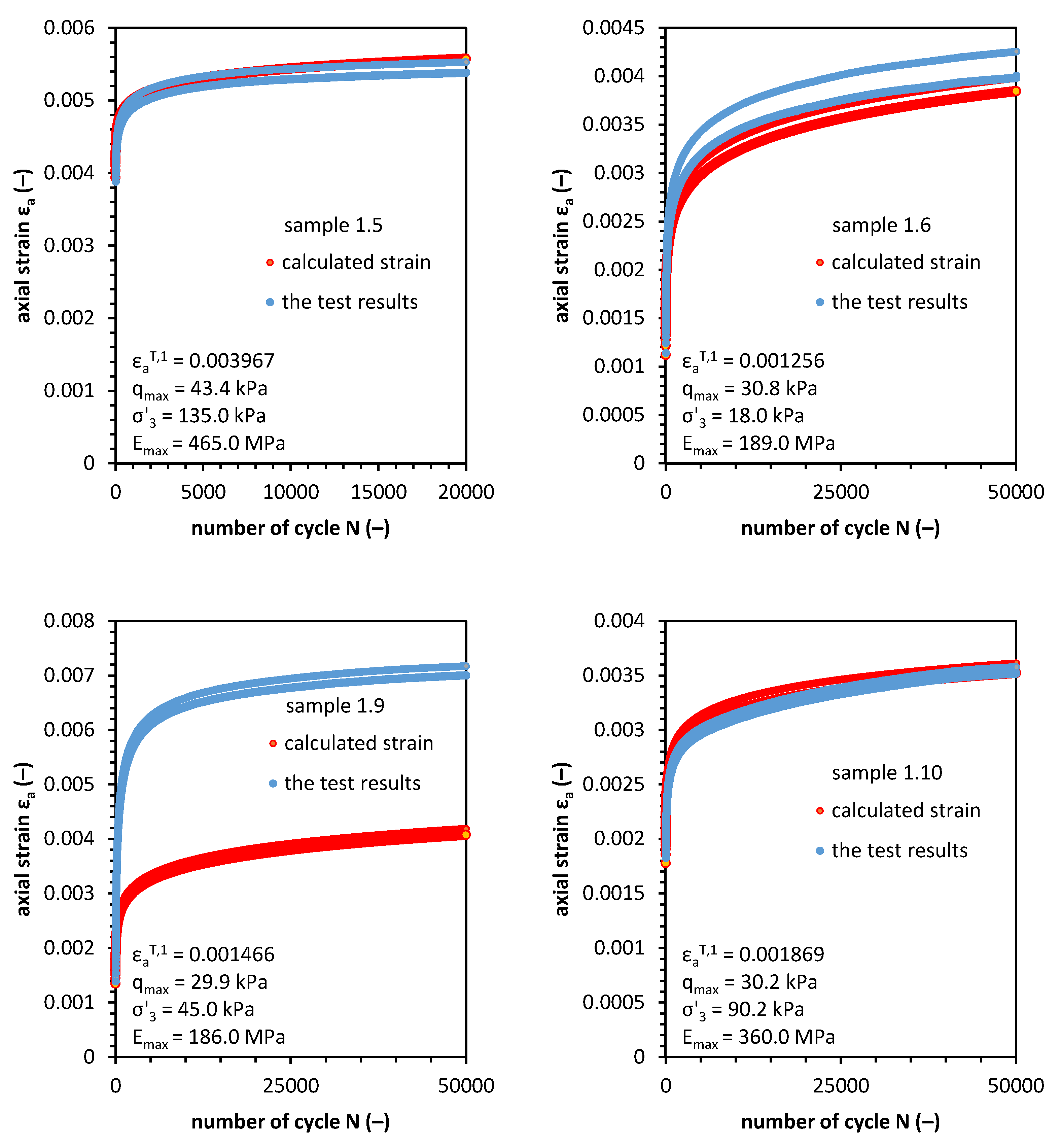
4.3. Model Validation

The presented results of the test show that the deformability of the soil can be described in terms of the equations derived from the previous considerations. We use undrained cyclic triaxial tests conducted on the samples presented in this study to derive model quality with ex–post evaluation. For calculations, the required data include the information about CSR, maximum shear modulus Emax and total strain in the first cycle caused by cyclic loading ε a T , 1 . The CSR is calculated here as the ratio of the maximal deviator stress qmax and the initial effective confining pressure σ’3. In total, four parameters are required to calculate the soil deformability in such conditions. Notably, the presented model uses the parameters which can be derived from the static triaxial tests.
Figure 13 presents the results of the cyclic triaxial test and the results of the total and plastic strain value calculations versus the number of cycles. We evaluated the SHLM quality of strain forecasting with the use of ex–post methods. In order to do so, we used cycle 10,000 as a reference. In Table 3, the data concerning the value of strain in the 10,000th cycle are presented. The ex–post analysis answers the question of how well the model would perform if it was used before the tests. This approach helps us to evaluate model reliability.
Based on the calculations performed in Table 3 the SHLM percentage error was between 0.0% and 51.72%. These values concern the 10,000 cycle. For the error of the whole model, the mean error (ME), mean percentage error (MPE), mean absolute error (MAE), mean absolute percentage error (MAPE) and Theil index values are presented in Table 4.
The ME and MPE show that the SHLM will deliver the strain value with 12.18% error and this value should be accounted as the standard error of model prognosis. The MAE gives information about the absolute error after 10,000 cycles. The conclusion can be made that for every 10,000 cycles, the value prognoses might be different according to the MAE value. Finally, we calculated the Theil parameter I2 in order to estimate the relative error of the model results. The Theil parameter can be decomposed into three categories, I12, I22 and I32. The first parameter shows how well the model delivers the value of the empirical data. The second parameter gives information on how precise the prognosis is, and the third parameter shows if the direction of the change was calculated properly. The Theil parameter value shows a high model prognosis in comparison with the test results. The peak value from which the Theil parameter is composed comes from the third part which refers to the direction of calculations, which is a flaw of SHLM, but because the model prognosis is precise with the strain characteristics, the SHLM can be employed with success in geotechnical engineering.
To compare the calculations with the SHLM, we derived constants for the Barksdale [11], Sweere [12,13] and Paute et al. [14,15] models for the samples in this study and we compared them with the test results. Figure 14 presents the abovementioned comparison. The constants for the Barksdale model are a = 0.0027, b = 0.0003, for the Sweere model a = −2.4897, b = 0.000064694, for the Paute et al. model a = 47.8047, b = −0.000006078. As it is easy to note, the SHLM gives the best fit to the data. The Barksdale and Paute et al. models overestimate the plastic strain over ten times and the Sweere model overestimates the plastic strain by more than one hundred.

5. Conclusions

In this paper, the results of the cyclic triaxial test on compacted sandy clay specimens are presented and we propose the SHLM as a method of plastic and total strain calculation. Geotechnical engineers can use the SHLM with the input parameters obtained without cyclic tests and with the use of the knowledge about stress state in soil and initial stiffness properties and initial strain caused by rapid loading. The paper shows the investigation of the effect of cyclic loading through several tests on soil deformation response. Based on these results, the following conclusions may be presented:
  • During all tests, the axial strain follows the same pattern. The first few cycles constitute a major part of the registered deformations. After this event, the increase in axial strain is lower and the amount of accumulated plastic strain is lower with each cycle. This behavior was defined as abation, which means the accumulation potential during cyclic loading abates with the running test. Specimens under higher critical state ratios show greater accumulation of deformations.
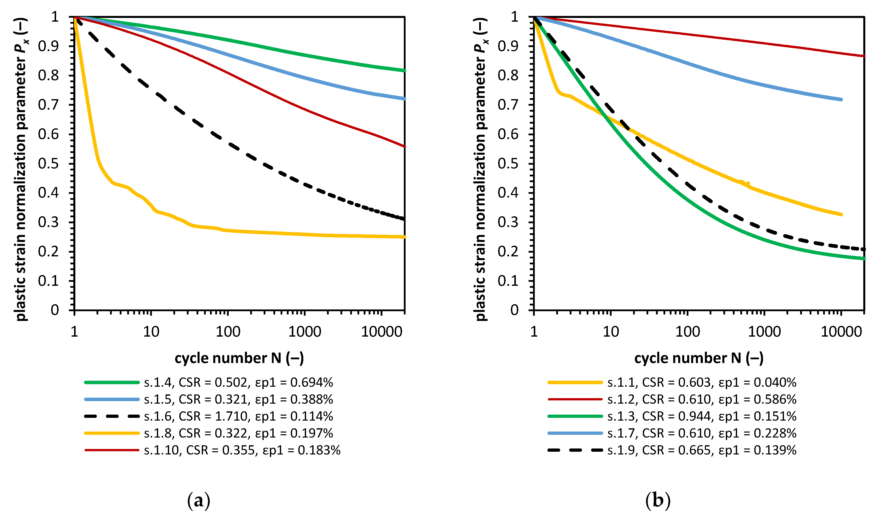
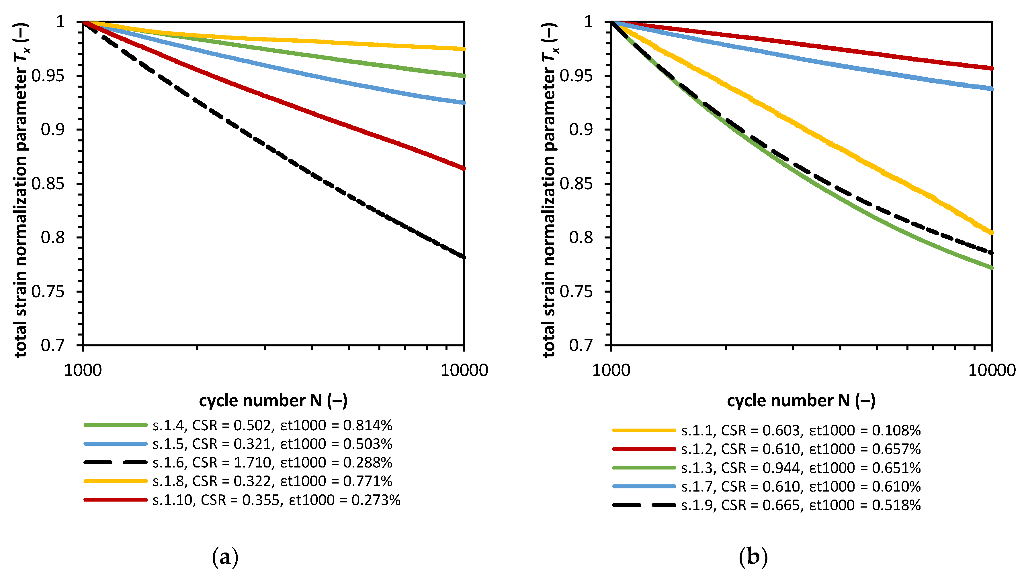
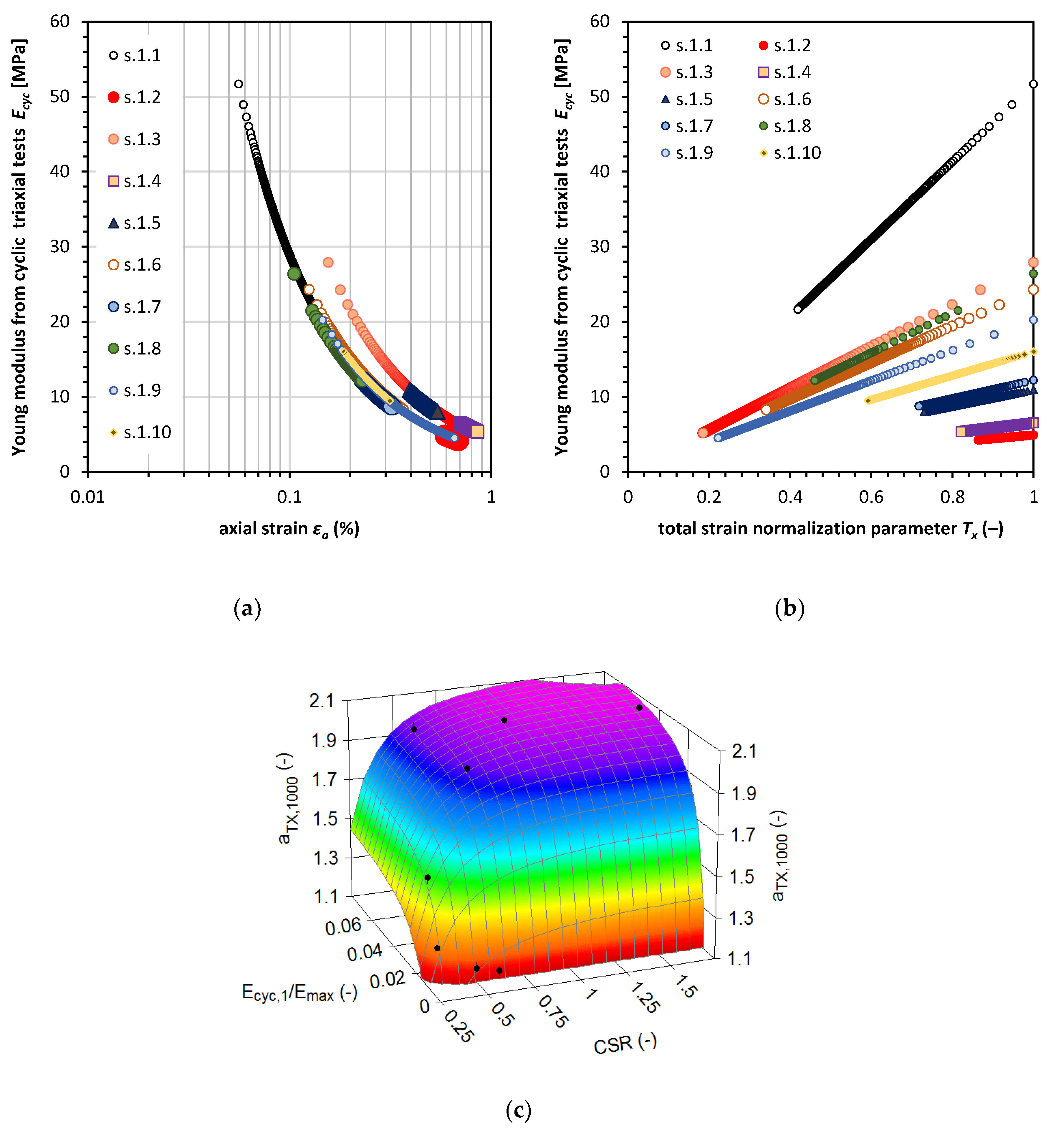
  • Registered strains were normalized with the use of first strain value as a reference. We introduced the total and plastic strain normalization parameters, and power function was employed to describe the strain–number of cycles relationship. This approach resulted in the sample stiffness analysis which showed a linear relationship between cyclic Young modulus Ecyc degradation and the total strain normalization parameter Tx.
  • The abation parameter Ax, which describes the plastic strain related to the total strain in one cycle, has shown satisfying linear relationship cyclic Young modulus degradation characteristics. This relationship also shows that the soil response to cyclic loading can be described in terms of abation rather than in terms of shakedown. Nevertheless, after numerous cycles, when the rate of plastic strain decreases to zero, the shakedown will occur and the soil respond to cyclic loading might be called as a shakedown
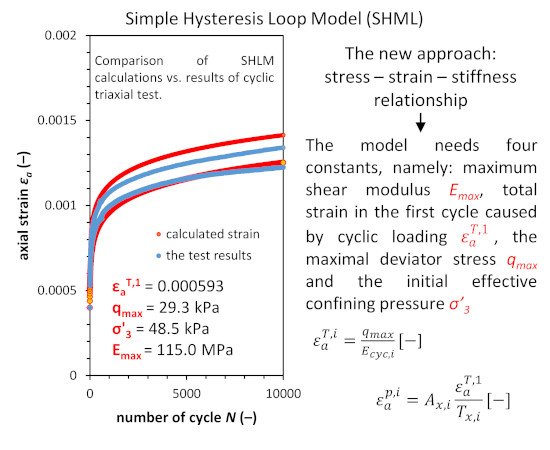
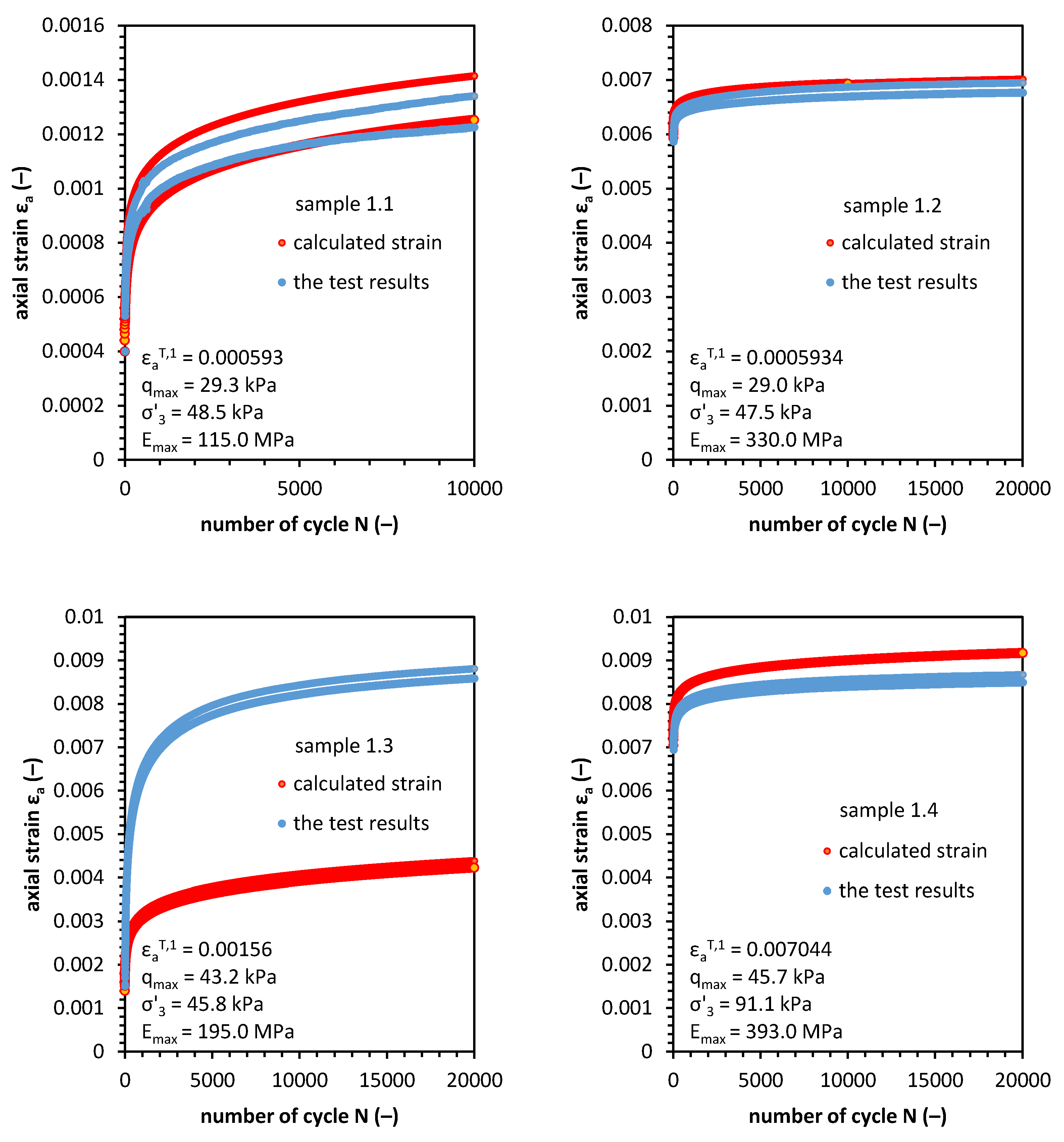
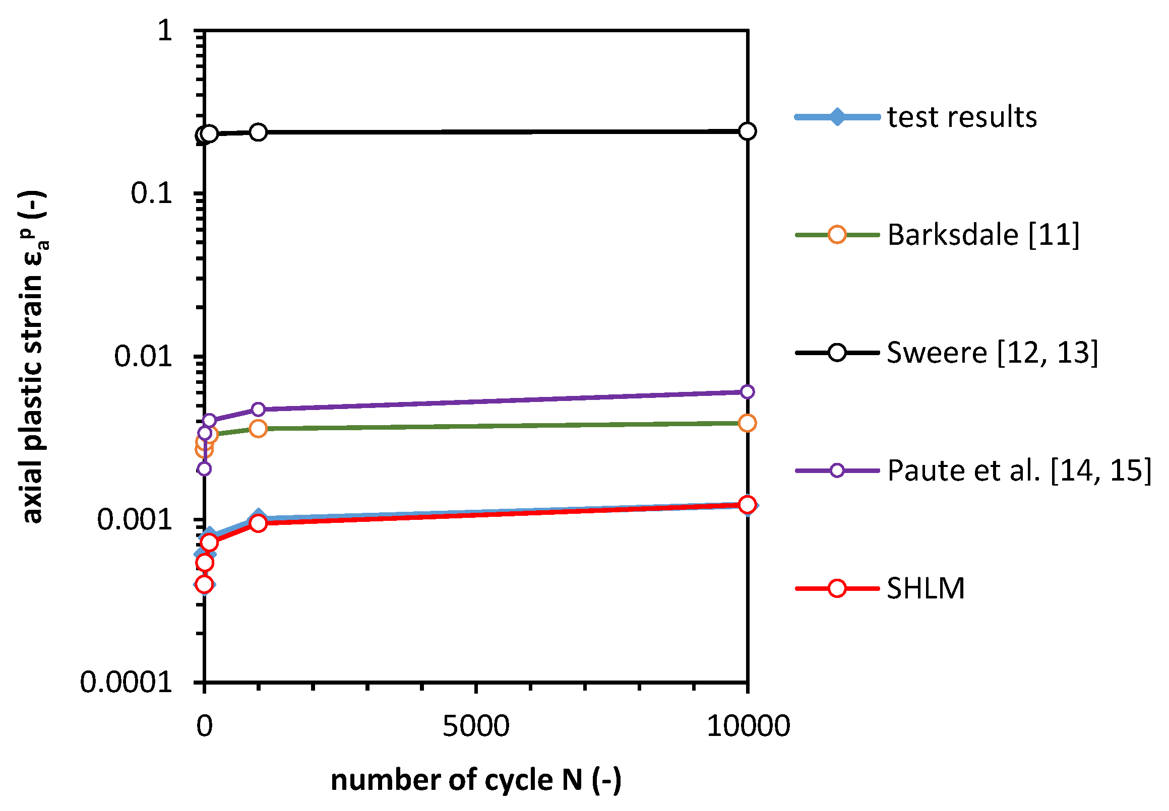
  • Based on the abovementioned stiffness–strain–stress considerations, we derived the SHLM. This model can simulate the strain development during cyclic loading and, therefore, enables engineers to model the soil deformation when subjected to cyclic loading. The model needs four constants, namely: maximum shear modulus Emax, total strain in the first cycle caused by cyclic loading ε a T , 1 , the maximal deviator stress qmax and the initial effective confining pressure σ’3. The SHLM is based on the six more hidden parameters which remain constant in this study and which might later be changed when more cyclic triaxial data would be employed for analysis. Nevertheless, the SHLM delivers a close forecast of plastic and elastic strain accumulation in terms of prognosis precision and quantity of strain accumulation. We estimated the mean percentage error of SHLM to be equal 12.18% based on ex-post analysis.
In the subject of strain modeling with permanent deformations, various models were developed to determine the relationship between accumulated strain and the number of cycles.
In most cases, the relationship was the power function or some modification of it. Studies have not examined the possible further deformation relationships to derive functional models independent from the obligation to perform the cyclic triaxial tests. In this study, we adopted a new perspective and the relationship between strain–stress and stiffness of soil was established. This resulted in the SHLM proposition independent from the duty of preliminary cyclic triaxial test execution and which adequately describes the response of cohesive soil to cyclic loading as abation.

Author Contributions

A.G. conceived and designed the experiments; A.G. and W.S. performed the experiments; A.G., wrote the paper; W.S. edited and audited the content. All authors have read and agreed to the published version of the manuscript.

Funding

This research received no external funding.

Conflicts of Interest

The authors declare no conflict of interest.

Appendix A

Table A1. The cyclic triaxial test loading program.
Soil Sample NoParameter Value, aPX (–)Parameter Value, bPX (–)Coeff. of Determination, R2
1.10.7475−0.09040.997
1.21.0238−0.01690.998
1.30.5030−0.11300.989
1.41.0100−0.02180.999
1.50.9943−0.03330.996
1.60.9189−0.11060.999
1.70.9276−0.02790.997
1.80.2750−0.00970.968
1.90.5423−0.10100.986
1.101.0613−0.06370.999
We performed the correlation analysis for the cycles 1000 to 10,000 because of the high plastic strain characteristic changes in the first few hundred cycles. The development was caused by the soil adjustment to cyclic loading and stabilization of the pore pressure. In 1000 cycles, the excess pore water pressure generates around 80% to 90% of its maximal value. Analysis of the contents of Table A1 in Appendix A shows a very high correlation of the power function with the cyclic triaxial test results.
Nevertheless, the aPX value should always be equal to 1.0 in the first cycle if the adapted function is going to model the Px change accurately. If the aPX parameter was fixed to 1.0, then the correlation in a few cases would be much smaller. The bPX parameter value was examined to establish a correlation with the soil properties. In Table A2, the Pearson correlation analysis result is presented.
Table A2. Pearson correlation analysis result for bPX parameter.
e (–)CSR (–)σ’3 (kPa)qm (kPa)qa (kPa)Δε1 (–)Δε10 (–)bPX (–)
R (–)0.316
0.373
0.819
0,003
0.355
0.344
0.047
0.897
0.484
0.157
0.068
0.982
0.008
0.982
0.381
0.277
e (–) 0.373
0.228
0.295
0.408
0.211
0.559
0.016
0.965
0.499
0.142
0.452
0.190
0.171
0.636
CSR (–) 0.752
0.012
0.096
0.793
0.346
0.328
0.188
0.603
0.335
0.345
0.658
0.039
σ’3 (kPa) 0.472
0.168
0.245
0.495
0.194
0.591
0.348
0.324
0.576
0.081
qm (kPa) 0.851
0.002
0.168
0.643
0.129
0.723
0.025
0.946
qa (kPa) 0.161
0.656
0.098
0.789
0.179
0.621
Δε1 (–) 0.952
0.000
0.280
0.434
Δε10 (–) 0.538
0.108
The underlined number stated for linear correlation as the coefficient of determination R2, the not underlined numbers are the P–values where for the P greater than 0.050, there is no significant relationship between two variables.
In Table A2, in the case of the bPX parameter, only the CSR shows the relationship equal to −0.658. For the linear regression, the coefficient of determination R2 is equal to 0.432, which shows a frail form of regression between the parameters. The results of aTX,1 and bTX,1 and bTX,1000 parameters calculation based on nonlinear regression analysis are presented in Table A3.
Table A3. The value of the aTX,1 and bTX,1 and bTX,1000 parameters based on nonlinear regression analysis.
Soil Sample NoTx,1000Tx,1
Parameter Value, aTX,1000 (–)Parameter Value, bTX,1000 (–)Coeff. of Determination, R2 (–)Parameter Value, aTX,1 (–)Parameter Value, bTX,1 (–)Coeff. of Determination, R2 (–)
1.11.9389−0.09510.9991.01955−0.096320.999
1.21.1479−0.01980.9991.021349−0.018030.994
1.32.0554−0.107570.9890.57083−0.159210.945
1.41.1653−0.022280.9991.017794−0.023360.998
1.51.2559−0.03350.9961.018177−0.036710.995
1.62.0787−0.106420.9990.949901−0.111880.999
1.71.2040−0.027290.9970.959363−0.032090.984
1.81.0582−0.008990.9680.546481−0.019590.526
1.91.9281−0.098630.9860.827068−0.148350.949
1.101.5347−0.062290.9991.076369−0.064990.998
We can observe a very high correlation of the power function with the cyclic triaxial test results. The bTX,1 and the bTX,1000 values are close to each other in cases when the aTX.1 is close to 1.0 and the R2 is higher than 0.980. For the three values, the aTX.1 is different from 1.0 and, interestingly, the product of aTX,1 and bTX,1 reduces the difference between the bTX,1 and the bTX,1000. The statistical analysis of the Pearson correlation analysis result is presented in Table A4.
Table A4. Pearson correlation analysis result for aTX and bTX parameters.
e (–)CSR (–)σ’3 (kPa)qm (kPa)qa (kPa)aTX,1000 (–)bTX,1000 (–)
R (–)−0.316
0.373
−0.819
0,003
0.355
0.344
0.047
0.897
−0.484
0.157
−0.395
0.259
0.369
0.294
e (–) 0.373
0.228
−0.295
0.408
−0.211
0.559
−0.016
0.965
0.223
0.535
−0.176
0.626
CSR (–) −0.752
0.012
−0.096
0.793
0.346
0.328
0.673
0.033
−0.642
0.045
σ’3 (kPa) 0.472
0.168
0.245
0.495
−0.604
0.064
0.579
0.079
qm (kPa) 0.851
0.002
−0.053
0.886
0.041
0.909
qa (kPa) −0.162
0.656
−0.157
0.665
aTX (–) -0.998
0.000
The underlined number stated for linear correlation as the coefficient of determination R2, the not underlined numbers are the P–values where for the P greater than 0.050, there is no significant relationship between two variables.

Appendix B

The calculation example, of the foundation settlement based on the 2:1 stress distribution method which is a prevalent empirical approach based on the assumption that the area over which the load acts increases systematically with depth [50]. The principle of the method is presented in Figure A1.
Figure A1. Schema of the approximate method for distribution of vertical stress due to surface load.
Applsci 10 02029 g0a1
If we consider the footing loaded with cyclic force P1 = 400 kN and with the amplitude Pa = 30 kN as a result of the rotating machine of other cyclic events. The resulting force P is equal to 430 kN. The footing has width B = 2.0 m and length L = 5.0 m. Therefore, the stress beneath the foundation σz=0m = 43 kPa. The cohesive soil which constitutes the foundation subgrade properties is presented in Figure A2.
Figure A2. Schema of the approximate method for distribution of vertical stress due to surface load.
Applsci 10 02029 g0a2
Based on the 2:1 stress distribution method, the stress from the footing in the cohesive soil is calculated. The settlement calculation was divided into 0.2 m slices for cohesive soil and the input parameters were assumed based on the triaxial test results presented in this study. The results of such an approach are presented in Table A5. In this example, the maximal Young modulus increases by 5 MPa with the 0.2 m depth. Among the SHLM parameters, the additional parameters are given, which are as follows: α, β and γ, which enable us to calculate the aTX, 1000 parameter, βTX, 1000 parameter, which is equal to −0.147, and Δa and Δb parameters, which enable us to calculate the αAX parameter, respectively. These parameters have no physical interpretations and they are derived for tested soil. With the increase in cyclic triaxial test results database, those parameters might be defined and they can differ among various cohesive soil types (for example, the plasticity index or soil gradation composition might be the difference factor) or they might be set to be constant based on the statistical analysis. The parameter value is presented in Table A6.
Table A5. SHML input parameters in the footing settlement calculations.
z (m)σmax = qmax (kPa)Emax (MPa)σ’3 (kPa)εaT,1 (–)
0.0–0.243.0300.045.00.005
0.2–0.437.6305.047.70.0045
0.4–0.633.2310.050.30.004
0.6–0.829.5315.053.00.0035
0.8–1.026.5320.055.70.003
1.0–1.223.9325.058.30.0025
Table A6. SHML constants for the footing settlement calculations.
ParameterαβγβTX,1000ΔaΔb
Value (–)2.07960.1004190.003034−0.147−175.883−23211.4
Based on the input parameters and constants, we can calculate the rest of the SHLM parameters by using the Equations (18) and then (19) to calculate Tx,i for N = I (Equation (21)) and Equation (24) for αAX value calculation to calculate the Ax parameter as in Equation (23). The results of the calculation are presented in Table A7.
Table A7. SHML parameters calculated based on input parameters and constants for the footing settlement calculations.
z (m)aTX,1000 (–)bTX,1 (–)αAX (–)
0.21.402216−0.04969−0.00032
0.41.453458−0.05497−0.00044
0.61.505418−0.06013−0.0006
0.81.557821−0.06516−0.00085
11.61031−0.07003−0.00125
1.21.6624−0.07471−0.00186
The total settlement in each layer ΔsaT,i was calculated based on the Equations (22) and (25) which are incorporated into Equation (A1):
s a T , i = z a , i σ m a x E c y c , 1 N i b T X , 1000 [ ] ,
The permanent settlement ΔsaP,i is calculated by using the Equation (25) which is as follows in Equation (A2):
s a P , i = z a , i ( N i b T X , 1000 1 a + b ( ε a T , 1 ) 3 + 1 ) ε a T , 1 N i b T X , 1000 [ ] ,
The following procedure has led to total and permanent settlement calculation, the results of which are presented in Table A8. In the given example, the cohesive soil layer with the initial thickness equal to 1.2 m will settle by 5.2 mm in the first cycle of loading and after one million repetitions will settle by 11.8 mm.
Table A8. SHML settlement calculation results.
z (m)Cycle Number N (–)
11000000
200.1985320.197084
400.1988450.197533
600.1990940.197921
800.1992940.198264
1000.1994580.198573
1200.1995920.198856
∑ (m)1.19481.1882
Settlement (mm)5.211.8

References

  1. Bogusz, W.; Godlewski, T. Philosophy of geotechnical design in civil engineering—Possibilities and risks. Bull. Pol. Acad. Sci. Tech. Sci. 2019, 67, 289–306. [Google Scholar]
  2. Soból, E.; Sas, W.; Szymański, A. Scale Effect in Direct Shear Tests on Recycled Concrete Aggregate. Stud. Geotech. Mech. 2015, 37, 45–49. [Google Scholar] [CrossRef] [Green Version]
  3. Gabrys, K.; Sas, W.; Soból, E.; Głuchowski, A. Torsional Shear Device for Testing the Dynamic Properties of Recycled Material. Stud. Geotech. Mech. 2016, 38, 15–24. [Google Scholar] [CrossRef] [Green Version]
  4. Abdelkrim, M.; Bonnet, G.; de Buhan, P. A computational procedure for predicting the long term residual settlement of a plat-form induced by repeated traffic loading. Comput. Geotech. 2003, 30, 463–476. [Google Scholar] [CrossRef] [Green Version]
  5. Araya, A.A.; Huurman, M.; Molenaar, A.A.A. Integrating Traditional Characterization Techniques in Mechanistic Pavement Design Approaches; First Congress of Transportation and Development Institute (TDI): Chicago, IL, USA, 2011; pp. 596–606. [Google Scholar]
  6. O’Reilly, M.P.; Brown, S.F. Cyclic Loading of Soils; Blackie and Son: London, UK, 1991. [Google Scholar]
  7. Peralta, P.; Achmus, M. An experimental investigation of piles in sand subjected to lateral cyclic loads. In Proceedings of the Physical Modelling in Geotechnics, Two Volume Set; Informa UK Limited: Zurich, Switzerland, 2010; pp. 985–990. [Google Scholar]
  8. Sas, W.; Głuchowski, A.; Szynański, A. Behavior of recycled concrete aggregate improved with lime addition during cyclic loading. Int. J. GEOMATE 2016, 10, 1662–1669. [Google Scholar] [CrossRef]
  9. Cai, Y.; Gu, C.; Wang, J.; Juang, C.H.; Xu, C.; Hu, X. One-Way Cyclic Triaxial Behavior of Saturated Clay: Comparison between Constant and Variable Confining Pressure. J. Geotech. Geoenviron. Eng. 2013, 139, 797–809. [Google Scholar] [CrossRef]
  10. Cai, Y.; Sun, Q.; Guo, L.; Juang, C.H.; Wang, J. Permanent deformation characteristics of saturated sand under cyclic loading. Can. Geotech. J. 2015, 52, 795–807. [Google Scholar] [CrossRef]
  11. Gräbe, P.; Clayton, C.R.I. Effects of Principal Stress Rotation on Permanent Deformation in Rail Track Foundations. J. Geotech. Geoenviron. Eng. 2009, 135, 555–565. [Google Scholar] [CrossRef]
  12. Huang, M.S.; Li, J.J.; Li, X.Z. Cumulative deformation behaviour of soft clay in cyclic undrained tests. Chin. J. Geotech. Eng. 2006, 28, 891–895. [Google Scholar]
  13. Chai, J.; Miura, N. Traffic-Load-Induced Permanent Deformation of Road on Soft Subsoil. J. Geotech. Geoenviron. Eng. 2002, 128, 907–916. [Google Scholar] [CrossRef]
  14. Pasten, C.; Santamarina, J.C. Thermally Induced Long-Term Displacement of Thermoactive Piles. J. Geotech. Geoenviron. Eng. 2014, 140, 06014003. [Google Scholar] [CrossRef] [Green Version]
  15. Barksdale, R.D. Laboratory evaluation of rutting in base course materials. In Proceedings of the Third International Conference on the Structural Design of Asphalt Pavements, Grosvenor House, Park Lane, London, UK, 11–15 September 1972. [Google Scholar]
  16. Lekarp, F.; Isacsson, U.; Dawson, A.R. State of the Art. I: Resilient Response of Unbound Aggregates. J. Transp. Eng. 2000, 126, 66–75. [Google Scholar] [CrossRef] [Green Version]
  17. Osouli, A.; Adhikari, P.; Tutumluer, E.; Shoup, H. Properties of aggregate fines influencing modulus and deformation behaviour of unbound aggregates. Int. J. Pavement Eng. 2019, 1–16. [Google Scholar] [CrossRef]
  18. Li, L.; Liu, J.; Zhang, X.; Li, P.; Saboundjian, S. Characterizing Permanent Deformation of Alaskan Granular Base–Course Materials. J. Mater. Civ. Eng. 2019, 31, 04019267. [Google Scholar] [CrossRef]
  19. Lal, M.H.; Noolu, V.; Pillai, R.J.; Kurre, P.; Praveen, G.V. A review on permanent deformation of granular material. Indian J. Public Heal. Res. Dev. 2018, 9, 1158. [Google Scholar] [CrossRef]
  20. Lekarp, F.; Dawson, A.R. Modelling permanent deformation behaviour of unbound granular materials. Constr. Build. Mater. 1998, 12, 9–18. [Google Scholar] [CrossRef]
  21. Sun, Q.; Dong, Q.; Cai, Y.; Wang, J. Modeling permanent strains of granular soil under cyclic loading with variable confining pressure. Acta Geotech. 2019, 1–13. [Google Scholar] [CrossRef]
  22. Gidel, G.; Hornych, P.; Chauvin, J.J.; Breysse, D.; Denis, A. A new approach for investigating the permanent deformation behaviour of unbound granular material using the repeated load triaxial apparatus. Bull. Liaison Lab. Ponts Chaussées 2001, 233, 5–21. [Google Scholar]
  23. Wang, H.-L.; Chen, R.; Qi, S.; Cheng, W.; Cui, Y.-J. Long-Term Performance of Pile-Supported Ballastless Track-Bed at Various Water Levels. J. Geotech. Geoenviron. Eng. 2018, 144, 04018035. [Google Scholar] [CrossRef]
  24. Wang, H.-L.; Chen, R.; Cheng, W.; Qi, S.; Cui, Y.-J. Full-scale model study on variations of soil stress in geosynthetic-reinforced pile-supported track bed with water level change and cyclic loading. Can. Geotech. J. 2019, 56, 60–68. [Google Scholar] [CrossRef]
  25. Trinh, V.N.; Tang, A.M.; Cui, Y.J.; Dupla, J.C.; Canou, J.; Calon, N.; Lambert, L.; Robinet, A.; Schoen, O. Mechanical characterisation of the fouled ballast in ancient railway track sub-structure by large-scale triaxial tests. Soils Found. 2012, 52, 511–523. [Google Scholar] [CrossRef]
  26. Wang, H.-L.; Cui, Y.-J.; Lamas-Lopez, F.; Dupla, J.-C.; Canou, J.; Calon, N.; Saussine, G.; Aimedieu, P.; Chen, R. Permanent Deformation of Track-Bed Materials at Various Inclusion Contents under Large Number of Loading Cycles. J. Geotech. Geoenviron. Eng. 2018, 144, 04018044. [Google Scholar] [CrossRef]
  27. Yu, H.S.; Khong, C.D.; Wang, J.; Zhang, G. Experimental evaluation and extension of a simple critical state model for sand. Granul. Matter 2005, 7, 213–225. [Google Scholar] [CrossRef]
  28. Yu, H.S. Plasticity and Geotechnics; Springer: New York, NY, USA, 2006. [Google Scholar]
  29. Konig, J.A. Shakedown of Elastic-Plastic Structures; Elsevier: Berlin, Germany, 1987. [Google Scholar]
  30. Werkmeister, S. Shakedown analysis of unbound granular materials using accelerated pavement test results from New Zeland’s CAPTIF facility. In Geotechnical Special Publication 154; Huang, B., Meier, R., Prozzi, J., Tutumluer, E., Eds.; ASCE: Shanghai, China, 2006; pp. 220–228. [Google Scholar]
  31. Werkmeister, S.; Dawson, A.R.; Wellner, F. Permanent Deformation Behavior of Granular Materials and the Shakedown Concept. Transp. Res. Rec. J. Transp. Res. Board 2001, 1757, 75–81. [Google Scholar] [CrossRef] [Green Version]
  32. Pande, G.N. Shakedown of Foundations Subjected to Cyclic Loads, Soil Mechanics-Transient and Cyclic Loads; Pande, G.N., Zienkiewicz, O.C., Eds.; John Wiley & Sons: New York, NY, USA, 1982; pp. 469–489. [Google Scholar]
  33. Boulbibane, M.; Ponter, A.R.S. The linear matching method for the shakedown analysis of geotechnical problems. Int. J. Numer. Anal. Methods Géoméch. 2006, 30, 157–179. [Google Scholar] [CrossRef]
  34. Werkmeister, S. Shakedown Analysis of Unbound Granular Materials using Accelerated Pavement Test Results from New Zealand’s CAPTIF Facility. Adv. Unsaturated Soil Seepage Environ. Geotech. 2006, 154, 220–228. [Google Scholar]
  35. Tao, M.; Mohammad, L.; Nazzal, M.D.; Zhang, Z.; Wu, Z. Application of Shakedown Theory in Characterizing Traditional and Recycled Pavement Base Materials. J. Transp. Eng. 2010, 136, 214–222. [Google Scholar] [CrossRef]
  36. Nega, A.; Nikraz, H.; Al-Qadi, I. Simulation of Shakedown Behavior for Flexible Pavement’s Unbound Granular Layer. Airfield Highw. Pavements 2015, 2015, 801–812. [Google Scholar]
  37. Soliman, H.; Shalaby, A. Permanent deformation behavior of unbound granular base materials with varying moisture and fines content. Transp. Geotech. 2015, 4, 1–12. [Google Scholar] [CrossRef]
  38. Melan, E. Zur plastizitat desraumlichen Kontinuums. Ing. Arch. 1938, 9, 116–125. [Google Scholar] [CrossRef]
  39. Koiter, W.T. General theorems for elastic-plastic solids. In Progressin Solid Mechanics; Sneddon, I.N., Hill, R., Eds.; North Holland Press: London, UK, 1960; pp. 167–221. [Google Scholar]
  40. Pham, C. Shakedown theory for elastic plastic kinematic hardening bodies. Int. J. Plast. 2007, 23, 1240–1259. [Google Scholar]
  41. Głuchowski, A.; Soból, E.; Szymański, A.; Sas, W. Undrained Pore Pressure Development on Cohesive Soil in Triaxial Cyclic Loading. Appl. Sci. 2019, 9, 3821. [Google Scholar] [CrossRef] [Green Version]
  42. Goldscheider, M.; Gudehus, G. Einige Bodenmechanische Probleme bei Küsten-und Offshore-Bauwerken. In Vorträge der Baugrundtagung; Deutsche Gesellschaft für Erd- und Grundbau: Nurnberg, Germany, 1976; pp. 507–522. [Google Scholar]
  43. Kenig, K. Litologia glin morenowych na Nizu Polskim-podstawowe metody badawcze. Biul. Panstwowego. Inst. Geol. 2009, 437, 1–57. [Google Scholar]
  44. Wang, H.-L.; Cui, Y.-J.; Lamas-Lopez, F.; Dupla, J.-C.; Canou, J.; Calon, N.; Saussine, G.; Aimedieu, P.; Chen, R. Effects of inclusion contents on resilient modulus and damping ratio of unsaturated track-bed materials. Can. Geotech. J. 2017, 54, 1672–1681. [Google Scholar] [CrossRef]
  45. Bajda, M.; Falkowski, T. Badania geotechniczne w ocenie budowy geologicznej fragmentu Skarpy Warszawskiej w rejonie ulicy Tamka. Landf. Anal. 2014, 26, 77–84. [Google Scholar] [CrossRef]
  46. Rudolph, C.; Bienen, B.; Grabe, J. Effect of variation of the loading direction on the displacement accumulation of large-diameter piles under cyclic lateral loading in sand. Can. Geotech. J. 2014, 51, 1196–1206. [Google Scholar] [CrossRef]
  47. Seed, H.B.; Martin, P.P.; Lysmer, J. The Generation and Dissipation of Pore Water Pressures during Soil Liquefaction; Report No. UCB/EERC-75/26; Earthquake Engineering Center, University of California: Berkeley, CA, USA, 1975. [Google Scholar]
  48. Idriss, I.M.; Dobry, R.; Sing, R.D. Nonlinear behavior of soft clays during cyclic loading. J. Geotech. Geoenviron. Eng. 1978, 104, 14265. [Google Scholar]
  49. Zhou, J.; Gong, X. Strain degradation of saturated clay under cyclic loading. Can. Geotech. J. 2001, 38, 208–212. [Google Scholar] [CrossRef]
  50. Fang, H.Y. Foundation Engineering Handbook; Springer Science & Business Media: New York, NY, USA, 2013. [Google Scholar]
Figure 1. Shema of stress-strain response of a material to cyclic loading, A—pure elastic response, B—shakedown, C—ratcheting during the cyclic loading.
Applsci 10 02029 g001
Figure 2. Soil respond to repeating loading in strain-controlled test (a) and stress-controlled test (b).
Applsci 10 02029 g002
Figure 3. Schema of dissipated energy and elastic strain energy in one cycle.
Applsci 10 02029 g003
Figure 4. Schema for abation parameter Ax parameters calculation.
Applsci 10 02029 g004
Figure 5. Cohesive soil physical properties, the results of the granulometric study (a), the result of the Proctor test (b).
Applsci 10 02029 g005
Figure 6. Results of the static triaxial tests on silty sandy clay samples, stress paths (a), normalized pore water pressure characteristics (b), and normalized Young modulus characteristics (c).
Applsci 10 02029 g006
Figure 7. Pore pressure ratio for the test results in confining pressure equal to 18, 90 and 135 kPa (a), and for the samples consolidated with confining pressure equal to 45 kPa (b).
Applsci 10 02029 g007
Figure 8. Plastic strain normalization parameter in confining pressure equal to 18, 90 and 135 kPa (a), and for the samples consolidated with confining pressure around to 45 kPa (b).
Applsci 10 02029 g008
Figure 9. Total strain normalization parameter in confining pressure equal to 18, 90 and 135 kPa (a), and for the samples consolidated with confining pressure at around 45 kPa (b).
Applsci 10 02029 g009
Figure 10. Total strain normalization parameter in reference to cycle 1000 Tx,1000 in confining pressure equal to 18, 90, and 135 kPa (a), and for the samples consolidated with confining pressure at around 45 kPa (b).
Applsci 10 02029 g010
Figure 11. Total degradation of Young modulus in cyclic loading Ecyc versus axial strain (a), and versus total strain normalization parameter Tx (b), the relation between the aTX parameter and the normalized cyclic Young modulus Ecyc/Emax. (c) the impact of the normalized Young modulus and cyclic stress ratio (CSR) on the aTX,1000 parameter value.
Applsci 10 02029 g011
Figure 12. The abation parameter characteristics: (a) the abation parameter Ax relationship to cyclic Young modulus Ecyc (b) and the relation between the abation constant and total strain in the first cycle of loading (b).
Applsci 10 02029 g012
Figure 13. Results of ex–post axial total and plastic strain calculations as a function of a number of cycles.
Applsci 10 02029 g013aApplsci 10 02029 g013b
Figure 14. Comparison between the test results and the plastic strain models for sample 1.1.
Applsci 10 02029 g014
Table 1. Soil index properties for the samples in cyclic triaxial test.
Soil Sample NoMoisture Content, w (%)Dry Density, ρd (g/cm3)Void Ratio, e0 (–)Shear Modulus, Gmax (MPa)
1.113.761.9320.391115.0
1.212.811.9720.358110.0
1.313.581.9040.38365.0
1.412.771.9840.324131.0
1.513.581.9480.366155.0
1.613.491.8970.38763.0
1.713.271.8920.370
1.813.811.7970.390
1.915.531.8410.33262.0
1.1016.371.9350.323120.0
Table 2. The cyclic triaxial test loading program.
Soil Sample NoMaximal Deviator Stress, qmax (kPa)Minimal Deviator Stress, qmin (kPa)Mean Deviator Stress, qm (kPa)Deviator Stress Amplitude, qa (kPa)Effective Confining Pressure, σ’3,0 (kPa)Cyclic Stress Ratio, CSR (–)
1.129.323.726.52.848.50.603
1.229.023.726.42.647.50.610
1.343.235.339.34.045.80.944
1.445.737.441.54.291.10.502
1.543.435.039.24.21350.321
1.630.822.826.84.0181.710
1.728.223.125.62.646.20.610
1.829.423.126.23.291.50.322
1.929.924.527.22.7450.665
1.1030.224.527.42.990.20.335
Table 3. Ex–post analysis of the 10,000th cycle: error and percentage error calculation results.
εaT,10000 Test (–)εaT,10000 Prognosis (–)Sample No.Error (–)Procentage Error (%)
0.001340.001391.1−0.00005−4.06%
0.006870.007051.2−0.00018−2.62%
0.008440.004071.30.0043651.72%
0.008570.008891.4−0.00032−3.71%
0.005440.005321.50.000122.21%
0.003680.003351.60.000339.05%
0.006590.003641.90.0029644.83%
0.003160.003361.10−0.000200.00%
Error is the difference between the test result and prognosis, Error = (εaT,10000 test) – (εaT,10000 prognosis).
Table 4. Ex-post analysis results for the Simple Hysteresis Loop Model (SHLM) error calculations and Theil parameter values.
IndexValue
ME0.00087
MPE12.18%
MAE0.001066
MAPE15.57%
I20.0976
I1221.41%
I221.23%
I3276.83%

