Review

Transfer Learning with Convolutional Neural Networks for Diabetic Retinopathy Image Classification. A Review

Nova Information Management School (NOVA IMS), Universidade Nova de Lisboa, Campus de Campolide, 1070-312 Lisboa, Portugal
*
Author to whom correspondence should be addressed.
Appl. Sci. 2020, 10(6), 2021; https://doi.org/10.3390/app10062021
Submission received: 11 February 2020 / Revised: 9 March 2020 / Accepted: 13 March 2020 / Published: 16 March 2020
(This article belongs to the Special Issue Medical Artificial Intelligence)

Abstract

:
Diabetic retinopathy (DR) is a dangerous eye condition that affects diabetic patients. Without early detection, it can affect the retina and may eventually cause permanent blindness. The early diagnosis of DR is crucial for its treatment. However, the diagnosis of DR is a very difficult process that requires an experienced ophthalmologist. A breakthrough in the field of artificial intelligence called deep learning can help in giving the ophthalmologist a second opinion regarding the classification of the DR by using an autonomous classifier. To accurately train a deep learning model to classify DR, an enormous number of images is required, and this is an important limitation in the DR domain. Transfer learning is a technique that can help in overcoming the scarcity of images. The main idea that is exploited by transfer learning is that a deep learning architecture, previously trained on non-medical images, can be fine-tuned to suit the DR dataset. This paper reviews research papers that focus on DR classification by using transfer learning to present the best existing methods to address this problem. This review can help future researchers to find out existing transfer learning methods to address the DR classification task and to show their differences in terms of performance.

1. Introduction

Diabetes mellitus (DM) is a chronic, metabolic, clinically heterogeneous disorder in which prevalence has been increasing steadily all over the world [1]. It is estimated that 366 million people had DM in 2011; by 2030, this will have risen to 552 million [2]. DM is characterized by persistent hyperglycemia, which may be due to impaired insulin secretion, resistance to the peripheral actions of insulin, or both, which eventually leads to pancreatic beta-cell failure [3]. People living with DM are more vulnerable to various forms of both short- and long-term complications due to metabolic aberrations that can cause damage to various organ systems, leading to the development of disabling and life-threatening health complications, the most prominent of which are microvascular (retinopathy, nephropathy, and neuropathy) and macrovascular complications [4].
Diabetic retinopathy (DR) is one of the most common microvascular complications that is caused by DM, and it happens when the blood vessels inside the retina are affected by high blood levels [5]. DR can create some irreversible complications that can lead to blindness in many cases. The number of patients that suffer from DR was estimated at 126.6 million in 2010, and this number is expected to grow to 191 million by 2030 [6]. More than 2.6% of blindness worldwide happens because of DR [7]. This percentage corresponds to a significant number of persons whose quality of life is severely affected. Though the early diagnosis of DR can help prevent blindness [8], this is a challenging task. More in detail, the main challenge of early-detected DR is the workforce that is needed to examine the retina images to detect DR [9] because diabetic patients must be assessed by an ophthalmologist at least once a year to detect the early signs of DR. Therefore, a reliable detection technology is needed to assist health care personnel in analyzing DR. According to Wilkinson et al. [10], DR can be classified into five grades: grade 0 is normal with no sign of DR, grade 1 means the presence of mild DR, grade 2 means moderate, grade 3 means severe, and, finally, grade 4 is defined by new vessel proliferation, where risks of vision loss include bleeding into the vitreous and tractional retinal detachment. Figure 1 shows the different grades of DR.
Deep learning belongs to the broad family of machine learning methods [11]. Differently to traditional neural networks-based classifiers, deep learning builds classifiers with many hidden layers, aiming at identifying the salient low-level features of an image [12]. In the context of deep learning, transfer learning is a technique that exploits the usage of features that were learned by a network over a given problem to solve a different problem in the same domain. Transfer learning has many advantages. First, it saves computational time because, instead of training a new model from scratch, it makes use of the information that is already available from the last training process. Second, it extends the knowledge it acquired from previous models, and third, transfer learning is very useful when the size of the new training dataset is small. Transfer learning promises valuable contributions to the fields of computer vision, audio classification, and natural language processing.
There have been many attempts to automatize the image classification task—either to facilitate the process or to make it more accurate. One of the earliest attempts was the convolutional neural network (CNN), which was introduced by [13] for the image classification task.
In 2012, thanks to the work of Krizhevsky et al. [14], CNNs became the most popular technique for addressing the image classification problem. The authors achieved state-of-the-art performance in the ImageNet Large Scale Visual Recognition Challenge (ILSVRC) competition [15], outperforming other commonly used machine learning techniques. CNNs can be used in image classification, as well as natural language processing [16,17,18] and time series analysis [19,20]. In all of these cases, training the weights of the deep network from scratch requires a substantial amount of time and huge datasets (hundreds of thousands of images). These requirements make deep learning algorithms very challenging in the context of medical images where, typically, only a limited number of images are available. A lot of time and experience are required to annotate medical images, and that is where transfer learning can play a significant role: It allows for the use of a pre-trained architecture that was previously fitted to images of the same domain.
Thus, transfer learning is particularly suitable for addressing the DR classification domain, where there is a lack of images to accurately train a CNN from scratch.
Several studies have been done to classify DR by using CNN, either by using transfer learning or by introducing novel architectures [21,22,23,24,25], but to the best of our knowledge, there have not been any reviews that survey the existing transfer learning techniques to classify DR images. To answer this call, in this paper, we discuss state-of-the-art DR image classification models that use the transfer learning of deep CNNs. Moreover, we discuss some important open questions to better apply transfer learning in the DR domain.
More in detail, we discuss state-of-the-art models and techniques that were published from 2015 to mid-2019. We used the following descriptors: “diabetic retinopathy,” “convolutional neural networks,” “transfer learning,” and “image classification” to cover the primary studies that address the classification of DR images by using transfer learning. These keywords were entered into the most well-known academic databases, namely Scopus and PubMed.
Two filters were used to produce the results: The first filter excluded any paper that was not about DR, which reduced the results from 172 papers to 31 papers; the second filter excluded any paper that was not about transfer learning, which resulted in 18 papers that were about transfer learning applied to DR.
This paper is organized as follows: Section 2 gives an overview of a CNN structure. Section 3 discusses various CNN architectures that are commonly used in transfer learning. Section 4 provides a brief description of the main DR datasets that are available for public use. Section 5 provides a review of papers on the usage of transfer learning in classifying DR. Section 6 presents the discussion, while Section 7 presents open research questions. Finally, Section 8 concludes the paper.

2. Convolutional Neural Networks and Transfer Learning

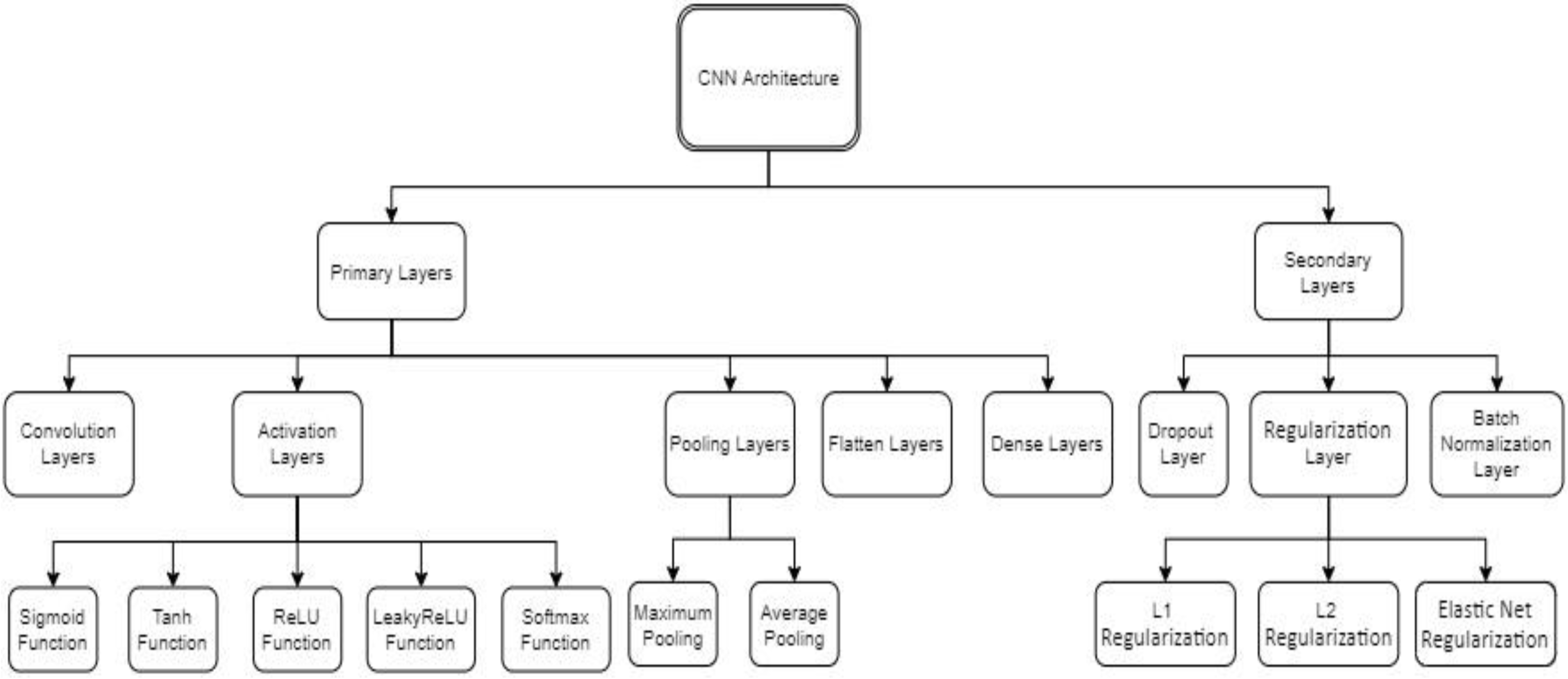
CNN layers can be classified into two categories: primary layers and secondary layers. The primary layers are the main layers that are used in the CNN and consist of convolution layers, activation layers, pooling layers, flatten layers, and dense layers. Secondary layers are optional layers that can be added to make CNNs more robust against overfitting and increase their generalizability. They include dropout layers, batch normalization layers, and regularization layers. Figure 2 shows a CNN structure.

2.1. Convolution Layers

The first and most important layer in a CNN is the convolution layer, which can automatically extract the image features without the need to manually define these features. The convolution layer can be defined mathematically by:
f ( g ( t ) ) = def f ( T ) g ( t T )   d T
where the convolution is the integral of the pointwise multiplication of two functions after one of them has been reversed and shifted [26]. From Equation (1), the g ( . ) function is the filter that is used. It is then reversed and slides along to the f ( . ) function, where f ( . ) is the input function. The area of the intersection between the two functions, g ( . ) and f ( . ) is the convolution value. In a CNN, the filters are not reversed but instead used as-is. The filter used, g ( . ) , can be expressed as a grid of order n . Usually, the numbers inside the filter are initialized randomly, and then these numbers are learned during the training process of the network. The result of the pointwise multiplication between the filter g ( . ) and the input function f ( . ) is saved in a new matrix called the output feature map. Figure 3 represents the differences between the convolution, the filter, and the output feature map.
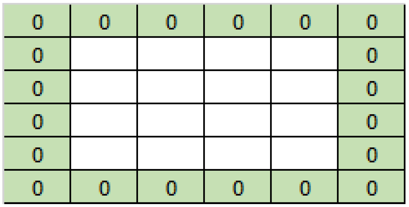
The steps that are performed by the filter function over the input function define the stride parameter. The stride can be formally defined as the amount by which the filter function g ( . ) moves at each step over the input function f ( . ) . Usually, after the convolution operation, the output feature map will have smaller dimensions than the input function. One can rely on the use of padding, a technique that adds zeroes around the input signal to maintain the original size, to maintain the dimensions of the output map and to prevent it from shrinking. Padding can be defined as the number of zeros that are added to the input function to control the spatial size of the output feature map throughout a network, especially deep networks. Figure 4 represents an input function with zero-padding. The convolution operation output depends on the input size, the used filter size, the used stride, and the padding. The output feature map size is calculated as follows:
O u t p u t   H e i g h t = H K + S + P S , O u t p u t   W i d t h = W K + S + P S
where filter size is K × K , input dimension is H × W , stride is S , and padding is P .

2.2. Activation Layers

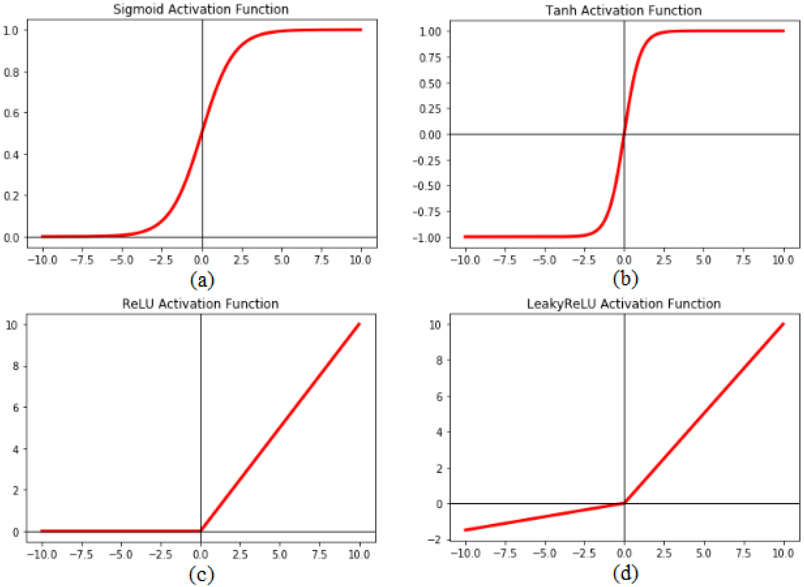
Activation layers, nonlinear layers that usually follow the convolution layers, play an important role as a selection criterion that decides whether a selected neuron will fire. The input of the activation layer is a real number that is transferred by the application of a non-linear function. The activation layer is important because it allows the network to learn nonlinear mappings to make it more robust against complex functions. The most common activation layers that are used in CNNs are sigmoid, Tanh, ReLU, LeakyReLU, and softmax. The activation layers can be classified into saturated activation layers and non-saturated activation layers. If the output of the activation layer ranges between finite boundaries, then it is classified as saturated; otherwise, if it tends to infinite, it is considered a non-saturated activation function. The non-saturated activation functions have many advantages compared to saturated activation layers. For instance, the non-saturated layers can significantly help in the exploding/vanishing gradient problem of the backpropagation algorithm [27], which is one of the main problems when training a CNN. Different activation functions are shown in Figure 5.

2.2.1. Sigmoid Function

A saturated activation layer, which is a different form of a logistic function where the input is a real number and the output is a number in the range of [0,1], can be defined by
f ( x ) = 1 1 + e x f ( x ) ( 0 , 1 )

2.2.2. Tanh Activation Function

The hyperbolic tangent function is a saturated activation layer that is commonly used when a negative gradient is important. It outputs a number in the range of [−1, +1]. The following formula defines it:
f ( x ) = e x e x e x + e x f ( x ) ( 1 , 1 )

2.2.3. ReLU Activation Function

The rectified linear activation layer [28] is considered one of the most important activation layers in a CNN. It is a non-saturated activation function that is mainly used to remove any negative values. It is very useful in a CNN because it eliminates any negative gradients when the threshold is at zero.
f ( x ) = max ( 0 , x )

2.2.4. LeakyReLU Activation Function

A leaky rectified linear activation layer [29] is a non-saturated activation function that allows some negative gradients to pass. It is used to reduce the effect of the negative gradients by factor α .
f ( x ) = { x ,   x > 0 α x ,   x < 0

2.2.5. Softmax Activation Function

Softmax is an activation layer that is usually at the end of a network, and it produces a discrete probability distribution vector.
P ( y = j | X ) = e x T w j k = 1 K e X T w k
where X is the input vector and w i is the predicted probability of y = j .

2.3. Pooling Layers

Pooling layers are usually between consecutive convolution layers to progressively reduce the spatial size of the representation to reduce the number of parameters and computation in a network. A pooling layer reduces the output feature map of the convolution layer by extracting important pixels and removing noise. In this work, we assumed that the measurements were not noisy, and, if this were not the case, a de-noising procedure would be necessary [30]. Additionally, a pooling layer is used to strengthen network spatial invariance [31]. The two main parameters of the pooling layers are the filter size and stride. The two main types of pooling layers are the maximum pooling layer and the average pooling layer.

2.3.1. Maximum Pooling

The pooling layer slides the filter over the output feature map of the previous convolution layer and keeps the maximum value of each grid.
f M P ( X ) = m a x i , j ( i , j )

2.3.2. Average Pooling

The pooling layer slides the filter over the output feature map of the previous convolution layer and takes the average of the grid.
f A P ( X ) = 1 n + m i = 1 n j = 1 m X ( i , j )

2.4. Flattening Layers

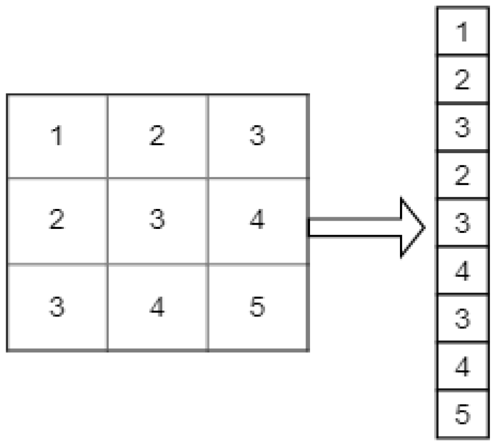
The output of the pooling layer is flattened to a 1 D vector because the subsequent dense layers can only receive 1 D vectors. A flattening layer can be seen in Figure 6. The dimensionality of the resulting vector is given by:
D i m F l a t = D i m i m g D i m i m g n u m c o l o r

2.5. Dense Layers

Dense layers, also known as fully connected layers, are usually placed at the end of a network, and they receive as input the output of the feature extraction layers. The main purpose of the dense layer is to consider all the features that were extracted from the previous layers and to use them to classify the original image. At the end of the network, a softmax or sigmoid function is applied to output the target probability.

2.6. Dropout Layer

A dropout layer is a regularization layer that was first introduced by [32]. It can be applied to any layer in the network. During network training, some neurons are disabled with a predefined dropout-rate probability P . It can be thought of as bagging for neural networks.

2.7. Regularization Layers

Complex models that have large weights usually have a low generalizability since these models can learn noise instead of learning the true model patterns [33]. Under the assumption that models with small weights have a better generalizability than those with large weights, regularization functions are commonly used to limit overfitting. Regularization works by adding a penalty term to the loss function to avoid large weights to be used by the model [34]. The main idea of regularization is to eliminate the weights that do not contribute to the model accuracy by shrinking them to zero. Three types of regularization have been introduced in the literature: L1, L2, and elastic nets. The main differences between these regularizations lie in the penalty terms.

2.7.1. L 1 Regularization

L 1 regularization constrains the weights to zero by adding the sum of the absolute values of the weights to the loss function. It can push some weights to be exactly zero and so can be thought of as a feature extractor. The magnitude of the penalty is determined by α , so the larger the value of α , the higher the constraint to the weights, usually 0 α 1 . L 1 regularization can be formally defined as:
f ( w ) = i = 1 n ( y i j = 1 m x i j w j ) 2 + α j = 1 m | w j |
where n is the number of training examples, m denotes the number of weights, w j is the weight at j neuron, y i is the label, and α is the regularization factor.

2.7.2. L 2 Regularization

L 2 regularization decreases large weights by adding the sum of the squares of the weights to the loss function. The magnitude of the penalty is determined by α , so the larger the value of α , the higher the constraint to the weights, usually 0 α 1 .   L 2 regularization can be formally defined as:
f ( w ) = i = 1 n ( y i j = 1 m x i j w j ) 2 + α j = 1 m w j 2
where n is the number of training examples, m denotes the number of weights, w j is the weight at j neuron, y i is the label, and α is the regularization factor.

2.7.3. Elastic Net Regularization

To overcome the shortcomings of both techniques, elastic net was introduced, as it linearly combines both regularization techniques to benefit from both techniques at once. Elastic net can be defined as:
f ( w ) = i = 1 n ( y i j = 1 m x i j w j ) 2 2 n + α ( 1 γ 2 j = 1 m w j 2 + γ j = 1 m | w j | )
where n is the number of training examples, m denotes the number of weights, w j is the weight at j neuron, y i is the label, α is the regularization factor, and γ is the mixing parameter between the ridge ( γ  = 0) and the lasso ( γ  = 1). By combining both L 1 and L 2 , the strength of each term can be tuned by α .

2.8. Batch Normalization Layers

Batch normalization can speed up the training of the network and increase its robustness against overfitting [35]. It reduces the network covariance shift [36]. Additionally, batch normalization adds noise to each layer to increase its robustness. It works by normalizing the inputs of each layer it is applied to by subtracting the batch mean and dividing by the batch standard deviation.
μ B = 1 n B i = 1 n B x ( i )   i s   t h e   m i n i b a t c h   m e a n
σ B 2 = 1 n B i = 1 n B ( x ( i ) μ B ) 2   i s   t h e   m i n i b a t c h   v a r i a n c e
x ^ ( i ) = x ( i ) μ B σ B 2 + ϵ   i s   t h e   s a m p l e   n o r m a l i z a t i o n
Z ( i ) = γ x ^ ( i ) + β   i s   t h e   b a t c h   n o r m a l i z a t i o n
where μ B is the mini-batch B mean, σ B is the mini-batch B standard deviation, n B is the number of instances in the mini-batch, x ^ ( i ) is the zero-centered and normalized input for instance i , γ is the scaling parameter for the layer, β is the shifting parameter (offset) for the layer, ϵ is a tiny number to avoid division by zero (typically 10 5 ; it is called a smoothing term), and Z ( i ) is the output of the B N operations (it is a scaled and shifted version of the inputs). Thus, in total, four parameters must be learned for each batch-normalized layer: γ   ( s c a l e ) ,   β   ( o f f s e t ) ,   μ   ( m e a n )   and   σ   ( s t a n d a r d   d e v i a t i o n ) .

2.9. Transfer Learning

Transfer learning is a deep learning technique that is used to rapidly and accurately train a CNN in which its weights are not initialized from scratch. Instead, they are imported from another CNN that was trained on a larger dataset. The most popular set of weights used for transfer learning is from the ImageNet dataset [37]. Several CNN architectures have been trained on the ImageNet dataset and have achieved a high accuracy. These weights can be used to classify another completely different dataset instead of randomly initializing the weights from scratch. There are four strategies in transfer learning. The first strategy is to remove the original fully connected layers that act as classifiers, freeze the entire network weights, use the CNN pre-trained layers as feature extraction, and then add a classifier layer such as a fully connected layer or another machine learning classifier, like a support vector machine. The second strategy is to remove the original fully connected layers, fine-tune the entire network weights by using a very small learning rate (LR), and add a new classifier layer that suits the new task. The third strategy is to remove the fully connected layers, fine-tune only the top layers while keeping the bottom layers frozen, and then add a new classifier layer that suits the new task. Many researchers have suggested that the bottom layers only detect generic features such as edges and circles, while the top layers detect more dataset-specific features. For this reason, many authors recommend only fine-tuning the top layers [38,39,40]. The fourth strategy is to use a state-of-the-art architecture and start training it from scratch, that is by using only the architecture that has been proven to work on different challenging datasets. A generic CNN model architecture can be seen in Figure 7.

3. CNN Architectures

In this section, the main CNN architectures used in transfer learning are reviewed. According to [41], the rise of deep learning in image classification started in 2012 by the introduction of AlexNet [14], which introduced the ReLU activation layer as well. The usage of a CNN in image classification increased its accuracy and eliminated the need to feature-engineer each image. After AlexNet, many architectures—namely VGG16, VGG19, ResNet, GoogLeNet, DenseNet, and Xception—were introduced with more features to efficaciously classify images.

3.1. VGG Network Architecture

In 2014, researchers at Oxford’s Visual Geometry Group introduced two novel architectures named VGG16 [42] and VGG19 [42]. VGG16 achieved a top five accuracy rate of 91.90% in the ImageNet competition in 2014. The VGG16 architecture has 138,355,752 parameters, five convolution blocks, and three dense layers. Each block contains some convolutional layers and then a max pool layer to decrease the block output size and remove the noise. The first two blocks have two convolutional layers each, and the last three blocks have three convolutional layers each. The size of the kernel that is used throughout this network has a stride of 1. After the five blocks, a flatten layer was added to convert the 3D vector of the blocks to a 1D vector to be inserted into the fully connected layers. The first two fully connected layers have 4096 neurons, and the last fully connected layer has 1000 neurons. After the fully connected layers, a softmax layer is inserted, and this is used to ensure that the probability summation of the output is one. The main difference between VGG16 and VGG19 is that VGG19 has 19 convolution layers instead of 16 convolution layers. The number of parameters increases from 138,357,544 to 143,667,240 because of additional layers. The authors argued that these additional layers make the architecture more robust and can learn more complex architectures.
The main benefit of this network is its sequential blocks, where the sequential convolutional layers that are inserted after each other allow for a reduction of the amount of spatial information needed. The main drawback of this network is that the authors specify more weights for the classifier portion and not to the feature extraction portion. This considerably increases the number of parameters. The network’s ImageNet weights are available in the Keras package.

3.2. ResNet Network Architecture

ResNet, which stands for residual network, was introduced by He et al. [43] in 2015 and achieved first place in the 2015 ImageNet competition with a top five accuracy rate of 94.29%. It has a total of 25,000,000 parameters. Compared to other architectures, ResNet is a very deep network that can reach up to 152 layers, and it has a unique connection called the residual connection, which is a connection that is applied between the convolutional layers and then passed to the ReLU activation layer. The residual connection makes sure that during backpropagation, the weights learned from the previous layers do not vanish. Three versions (which differ in the number of layers) of this network have been introduced, namely ResNet50, ResNet101, and ResNet152. The main benefit of this network is the use of residual connections, which makes it possible to use a large number of layers. Moreover, increasing the depth of the network (instead of widening it) results in fewer extra parameters. The main drawbacks of this network are the summation in each residual block, which makes the filter size the same. Additionally, this network requires large datasets to be properly trained, thus resulting in a computationally expensive training phase. The network’s ImageNet weights are available in the Keras package.

3.3. GoogLeNet Network Architecture

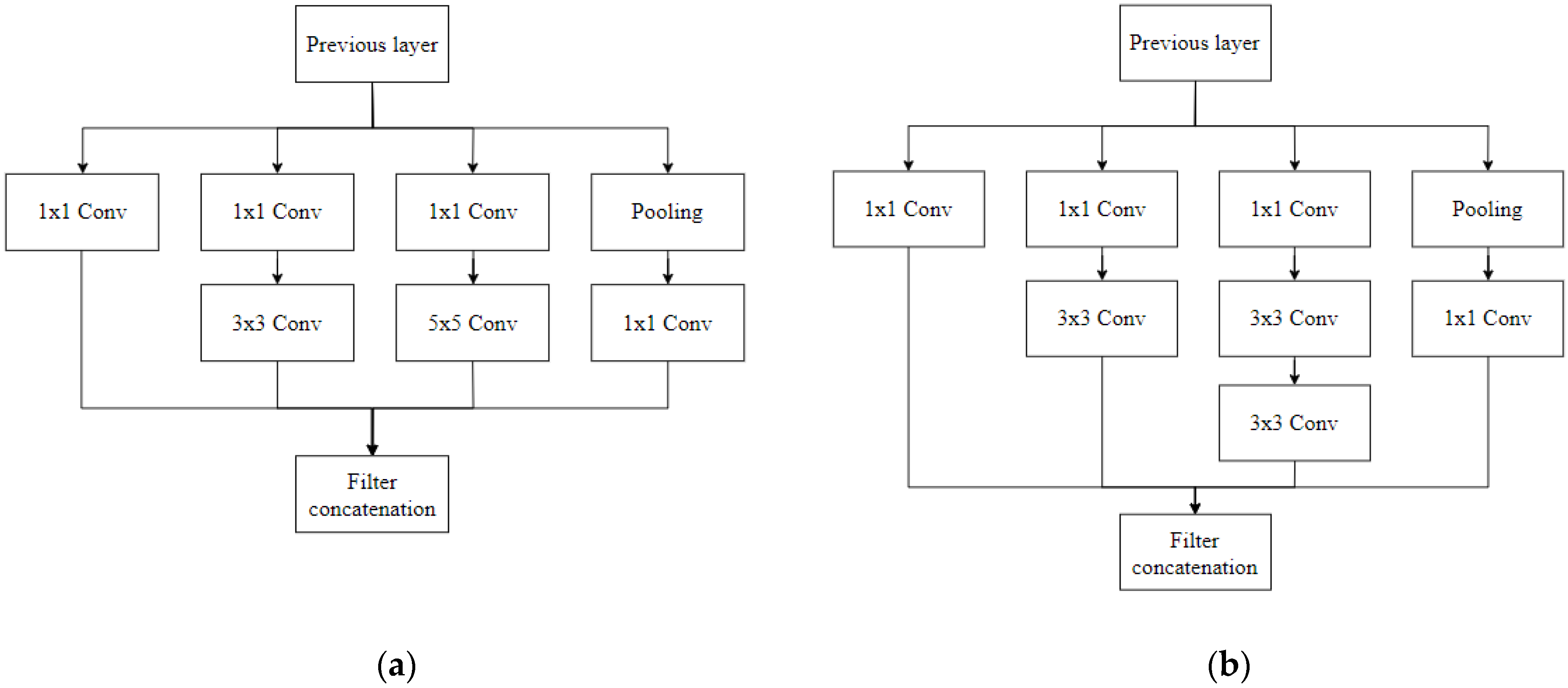
In 2014, Google researchers introduced a novel architecture called the GoogLeNet network [44], which is also known as IncpetionV1 architecture. The authors won the ImageNet competition [45] with a top 5 accuracy rate of 92.2%. After the success of InceptionV1, the authors introduced other versions like InceptionV2 and InceptionV3. The main idea of GoogLeNet architecture is to use multiple convolution layers in the same block to go not only deeper but wider and to capture different features of the images; these blocks are referred to as Inception blocks. The most popular GoogLeNet architectures are the InceptionV1 and InceptionV3 architectures. In the InceptionV1 inception blocks, six convolution layers are used, while in the InceptionV3 inception blocks, seven convolution layers are used. In the remainder of the paper, just like in the literature, the InceptionV1 architecture is referred to as the GoogLeNet architecture. The main benefit of this network is the presence of an inception module, which allows the network to capture different aspect ratios of the same image by using the convolution layers in parallel. The main drawback of this network is the computational effort that is needed to train it because the layers are deep and wide. The InceptionV3’s ImageNet weights are available in the Keras package. An InceptionV1 block and InceptionV3 block are shown in Figure 8.

3.4. AlexNet Network Architecture

AlexNet architecture [14] was the first CNN network to participate in the ImageNet challenge in 2012. It achieved an accuracy rate of 84.60%, which outperformed all the previous shallow algorithms used in image classification. Since then, CNNs have become the state-of-the-art algorithm in image classification. The AlexNet architecture has 60,000,000 parameters, five convolution layers, and three dense layers. The two-novel introductions in AlexNet were the usage of the ReLU activation function (instead of the sigmoid activation function) and the usage of dropout to overcome the overfitting that can be caused by this deep architecture. The main advantage of this network relies on the fact that the training process is computationally efficient compared with the other networks that have been taken into account. On the other hand, the network is not deep enough to capture complicated features from images.

3.5. DenseNet Network Architecture

DenseNet architecture [45] stands for densely-connected convolutional networks. It was inspired by ResNet, but instead of the residual connections, the authors proposed the use of dense blocks. The dense block consists of sequentially placed convolution layers, like VGG, but each layer has a connection to all the subsequent layers. The main idea is, for each convolution layer to receive the information from all the previous layers. DenseNet has 8,062,504 parameters and achieved a 93.34% top 5 accuracy rate on the ILSVCR challenge. The main advantage of this network is the presence of connections between all layers, which reduces the information loss between layers (especially the deep layers). The main drawbacks are the following: The training phase is computationally expensive, and it requires very large datasets to achieve satisfactory performance. The network’s ImageNet weights are available in the Keras package.

3.6. Xception Network Architecture

The Xception (which stands for extreme inception) network was introduced by Chollet [46], and it was inspired by the InceptionV3 architecture. The main idea that is exploited by the Xception architecture is to replace the inception module with depthwise separable convolution, followed by a pointwise separable convolution. This network is 71 layers deep, and it has 22.9 million parameters. The Xception network achieved a 94.50% top 5 accuracy rate on the ILSVCR challenge. The main advantage of this network is that it has a deep architecture but with a small number of parameters, thus making it computationally efficient compared to other deep networks. The main drawback is that this network requires very large datasets to be able to train all its parameters.
Table 1 shows a summary of the proposed networks with their number of parameters and their accuracy over the ImageNet dataset [37]. The accuracy is calculated by dividing the correctly classified observations over the total number of observations. The t o p k accuracy is the accuracy of the architecture over predicted labels y ^ , where the top 5 accuracy represents the accuracy over 5 classes accuracy and the top 1 accuracy represents the accuracy for a single-class classification. When k = 5 , the accuracy is measured by taking into account if the label y is present in the top 5 predicted labels y ^ , while if k = 1 , t o p k is the de-facto accuracy measure. The t o p k accuracy measure was used here because the ILSVRC challenge had 1000 classes.

4. DR Datasets

Several DR datasets were made publicly available to allow researchers to develop algorithms that are able to classify DR. A brief description of these datasets is given in this section. DR Datasets descriptions are shown in Table 2.

4.1. Kaggle Dataset

The Kaggle DR [47] dataset is considered one of the most important datasets for DR because it includes more than 88,000 publicly available images that were captured by using different cameras at different angles and dimensions. This dataset is divided into 40% for training and 60% for testing, and various cameras took the images. Therefore, different levels of quality appear in this dataset. The annotation of this dataset is a five-class annotation, as proposed by Wilkinson et al. [10]. The dataset suffers from imbalance, as the rare DR levels (3 and 4) cover less than 5% of the dataset.

4.2. Messidor Dataset

Messidor [48,49] is a publicly available dataset that consists of 1200 DR images. This dataset, like the Kaggle dataset, was acquired by using different cameras and settings, and it was built by collecting images from three different hospitals in France. This dataset is more balanced than Kaggle’s because each class is distributed uniformly. The DR grades are divided into four grades.

4.3. DR1 Dataset

DR1 [50] is a publicly available dataset that was provided by the Federal University of Sao Paulo, Brazil. The dataset contains 1014 images with 68% normal images and 32% DR images. All the images were captured by using the same camera.

4.4. E-ophtha Dataset

The E-ophtha dataset [51] is a publicly available dataset that contains two main subsets of images. The E-ophtha_Ex dataset has the objective of detecting exudates in fundus images. This dataset has 82 images split into 47 fundus images with exudates and 35 images without exudates. The other dataset is the E-ophtha_MA, and the objective of it is to detect microaneurysms in fundus images. This dataset contains 381 images divided into 148 images with aneurysms and 233 without arterial swelling.

4.5. STARE Dataset

The STARE dataset [52] is a publicly available dataset that contains 400 images that were captured by using the same camera. It has 397 fundus images divided into 14 retina-related diseases.

5. Paper Review

This section discusses the selected papers based on different aspects like the architecture used, the target dataset used, the optimizer used, and the LR used, the performance of the architecture after transfer learning, the fine-tuning process employed, and, finally, the validation process whenever applicable.
In transfer learning, a set of weights that were learned from an image dataset can be used to classify another image dataset. The deep layers are generic and can be used to extract salient features that are suitable for classifying any image. This aspect is why many authors have tried to use transfer learning in detecting DR. For instance, Gulshan et al. [53] used InceptionV3 architecture to classify DR into two grades: DR or No DR. The dataset that was considered by the authors contained 128,175 images. The reported results on two test datasets, with sizes 9963 and 1748, had sensitivities of 97.5% and 96.1%, respectively. Masood et al. [54] used the Kaggle dataset to assess the performance of the InceptionV3 model to classify DR into five grades. The authors chose 4000 images and cropped them to 500 pixels. The authors used accuracy to assess the model’s performance, which was reported as 48.8%.
Li et al. [55] discussed the usage of transfer learning for detecting DR by comparing different network architectures, including AlexNet, VGG-S, VGG16, and VGG19, to two datasets: the Messidor and DR1 datasets. Three transfer learning techniques were analyzed: fine-tuning the entire networks, fine-tuning the networks layer-wise, and, finally, freezing the weights of the entire network and applying SVM as a classification layer. The authors used a stochastic gradient descent for the optimizer, and the images were pre-classified as either DR or No DR to pose a binary classification problem. The accuracy measure used was the AUC of the ROC curve. The highest AUC achieved was obtained by fine-tuning the entire network, while the second-best performance was achieved by fine-tuning layer-wise. The VGG-S architecture obtained the highest AUC that was achieved for the Messidor dataset with an AUC of 98.34%. For the DR1 dataset, an AUC of 97.86% was obtained by using the same network.
Mohammadian et al. [56] compared the InceptionV3 and Xception architectures to classify DR into two grades, DR or No DR, by using the Kaggle dataset. The authors used the whole dataset of 35126 images, with 20% of the images being used to test the algorithm’s performance over unseen data. The authors fine-tuned the last two blocks of the two architectures and compared two optimizers with different LRs: stochastic gradient descent and Adam. The authors augmented the images by horizontally and vertically flipping the images or by shifting and rotating the images to increase the robustness of the model. The authors used the accuracy measure to assess the performance of the architectures. The reported results were 87.12% for the InceptionV3 architecture and 74.49% for Xception.
Takahashi et al. [57] trained a modified GoogLeNet architecture by using a private dataset. They used 9443 images to train the model and 496 to test it. They cropped the images to 1272 × 1272 pixels, and they considered a four-class classification scheme. The reported accuracy was 81%, and the kappa score was equal to 0.74. Choi et al. [58] investigated the impact of transfer learning on the STARE dataset [52]. They used image augmentation techniques to increase the size of the dataset to 10,000 images, with ten retina disorder categories, including DR. The authors opted for the pre-trained VGG19 and AlexNet architectures. An ensemble was created to increase the network accuracy, and K-fold validation with k = 5 was used to validate the results. The highest accuracy that was obtained by the authors was achieved by using VGG19 architecture with random forest (RF) as a classifier.
Wang et al. [59] investigated transfer learning techniques by using three network architectures: AlexNet, VGG16, and InceptionNetV3. The authors used 166 images from the Kaggle dataset to tune the algorithms. The authors opted for the five-stage classification approach instead of the binary classification approach that has been used by other authors for this specific dataset. Additionally, they employed a stochastic gradient descent optimizer with Nesterov momentum to accelerate the convergence to the minimum. The authors cropped the images for each architecture to 227 × 227 for AlexNet, 224 × 224 for VGG16, and 299 × 299 for InceptionV3. They used the accuracy of the network as the evaluation metric, and they used K f o l d   v a l i d a t i o n with K = 5 to cross-validate the results. The best-reported accuracy was 63.2% for the InceptionV3 architecture. Hazim et al. [60] used 580 images from the Messidor dataset to test the transfer learning of AlexNet. They opted for a two-class classification, and they cropped the images to 227 × 227 . They achieved an 88.3% accuracy on the test set, which consisted of 290 images.
Lam et al. [61] considered the sliding windows algorithm, where small patches from the original images are used to train the CNN. These patches contain the important features of each image, such as the presence of exudates or microaneurysms. The authors used the Kaggle dataset to extract these patches. They extracted 1324 patches from 243 images and split these patches into training and testing datasets. They tested the proposed algorithm by using the E-Optha dataset, which contained 195 images. They used GoogLeNet architecture to train the model with an input size of 128 × 128 . The authors considered a multi-class classification task with five DR grades. They resized the test images to 2048 × 2048 and normalized the pixels to test the model. Subsequently, the trained model crossed over the test image to produce a heat map with a probability score for every one of the five grades. The authors compared five pre-trained architectures (AlexNet, VGG16, GoogLeNet, ResNet, and InceptionV3) for binary classification and multi-class classification. The best performing architecture was InceptionV3 with a multi-class accuracy of 96% and a binary-class accuracy of 98%.
Lam et al. [62] trained a CNN by using transfer learning of the AlexNet, VGG16, and GoogLeNet models, and they utilized Kaggle two-class output. The authors reported that GoogLeNet achieved the highest sensitivity of 95% and specificity of 96%. The authors tried to utilize the multi-class Kaggle dataset, but they stated that a CNN cannot learn mild class sensitivity. The authors achieved decent results for detecting mild grades when using the Messidor dataset. Wan et al. [63] compared the difference between transfer learning and learning from scratch. The authors used four CNN architectures, namely AlexNet, ResNet, GoogLeNet, and VGG. The authors performed their experiments on the full Kaggle dataset, and they used the AUC of the ROC curve, accuracy, sensitivity, and specificity as evaluation criteria. The authors reported that transfer learning did significantly increase the performance of CNN, with VGG-S producing the highest AUC.
Xu et al. [64] studied the difference between the performance of DenseNet with and without fine-tuning. The authors examined their method on a private dataset with 10,000 images and five grades. The authors used image augmentation to increase the size of the dataset and to balance the dataset between different classes. The final dataset contained 20,000 images that were distributed equivalently between the five classes. The authors used a stochastic gradient descent (SGD) as an optimizer with an LR of 0.1 for training from scratch and an LR of 0.01 for fine-tuning the network. The authors reported that transfer learning increased the accuracy of the model used.
Tsighe et al. [65] investigated the usage of the InceptionV3 architecture to detect DR in the Kaggle dataset. The authors chose 2500 images and cropped them to 300 × 300 to train the model, and 5000 images were used to test the model. The authors pre-classified the images as either DR or No DR to make it a binary classification task. They employed a stochastic gradient descent as an optimizer, with an LR of 0.0005, to fine-tune the neural network. The reported result was a 90.9% accuracy and a 3.94% loss. Chen et al. [66] considered the pre-trained InceptionV3 architecture to classify DR on 7023 images of the Kaggle dataset. The authors adopted a five-stage classification approach with the quadratic weighted kappa as an accuracy measure. The images were cropped to 229 × 229 , and a stochastic gradient descent was used as an optimizer. Image augmentation was used with an early stop for 15 iterations to overcome the overfitting of the network. The reported Kappa score was 0.64, with an accuracy of 80%.
Zeng et al. [67] proposed a novel Siamese-like architecture in which left and right fundus images were classified together. Siamese neural networks are networks with two parallel neural networks, and each of these networks takes different inputs. The authors used the Kaggle dataset with 28,104 training images split between right and left eyes and 7024 to test the architecture. They used the pre-trained InceptionV3 network on the ImageNet dataset. The authors examined the five-stage classification, as proposed by Wilkinson et al. [10], and opted to use a binary class classification. They used Adam as an optimizer, quadratic weighted kappa as the accuracy measure for the multiclass classification, and the AUC of the ROC for the binary classification. All the layers of InceptionV3 were fine-tuned, and the images were cropped to 229 × 229 . The authors augmented images by randomly flipping them horizontally and by randomly applying a geometric transformation to increase the dataset’s size and to control overfitting. They normalized all images from [0,255] to [−1,+1]. They reported the kappa result as 0.829 for the multiclass classification and an AUC of 95.1% for the binary classification.
Zhang et al. [68] used a private dataset with 13,767 images to propose a model called DeepDR, which uses deep learning based on transfer learning models to detect DR. The model consists of three stages: identification, grading, and reporting. The identification stage is a binary classification model to predict the presence of DR. If DR exists, then the image is graded by using the grading stage of the four stages of DR; the last stage reports the result of the model. The authors used InceptionV3, Xception, and InceptionResNetV2 for feature extraction in the identification system. Moreover, they added a global average pooling layer to normalize the output of the feature extractor, and they subsequently added four dense layers with sizes 1024, 512, 256, and 128, respectively. A dropout layer between the dense layers, with a probability of 50%, was employed to limit overfitting. Due to its speed of convergence, the authors opted for the LeakyReLU activation function with a β of 0.2 and, in the end, a softmax layer to sum up the probabilities to 100%. For the grading system, the authors used ResNet50, DenseNet169, and DenseNet201 for feature extraction in the grading system. They then added a global average pooling layer and four dense layers with sizes 2048, 1024, 512, and 256, respectively. They employed a dropout layer between the dense layers with a probability of 50%, LeakyReLU, as the activation function for all the dense layers with β of 0.2 and, in the end, the softmax layer. The authors averaged the outputs of the softmax layer of the three models to decrease the variance of the model output. The identification model achieved a sensitivity of 97.5% and a specificity of 97.7%, while the grading model reached 98.1% for sensitivity and 98.9% for specificity.
Yip et al. [69] explored three CNN architectures, namely VGG, ResNet, and an ensemble of both architectures. The authors experimented with using a private dataset with three classes of DR and with 148,266 images divided into 51.5% to train and 48.5% to validate the model. Three measures were used to assess the quality of the model, namely AUC, sensitivity, and specificity. The authors reported that transfer learning increased model accuracy. Gao et al. [70] used a private dataset with 4476 images with four classes. The authors cut the original images into four 300 300 partitions that were the input of four InceptionV3 networks, and then they concatenated the results to a single layer. The original fully connected layers were removed, and only a softmax layer was used. The Adam optimizer was employed to fine-tune the InceptionV3 networks. The authors compared their method against ResNet18, ResNet101, VGG19, and InceptionV3. The reported results showed that their model achieved a higher accuracy than the other models. Table 3 shows the list of the reviewed papers that applied transfer learning to classify DR.

6. Discussion

This study reviewed recent studies that implemented transfer learning in classifying diabetic retinopathy images. These studies were extracted from two databases (PubMed and Scopus), and, after applying two filters, 18 studies were selected. The selected papers were analyzed based on six aspects: the architecture used, the target dataset used, the optimizer used, the LR used, the performance of the architecture after transfer learning, the fine-tuning process used, and, finally, the validation process that was applied. In this section, we discuss the main findings of this analysis.

6.1. Architectures Used

In the reviewed articles, many state-of-the-art architectures were used to classify DR. Among them, InceptionV3 was the most commonly used, followed by the AlexNet and VGG16 architectures. The choice of the architectures did not depend on the size of the dataset. In studies [55,56,58,59,61,62,63,68,69,70], the authors compared different architectures to determine the best performing one. In studies [56,59,61,63,70], the authors compared InceptionV3 architecture to other networks, and InceptionV3 achieved the best performance in all the studies except for [63]. The lowest performance was achieved by the AlexNet architecture in the following studies: [58,59,61,62,63]. The high performance of InceptionV3 may be attributed to the inception module used. This module can capture different aspect ratios in the same image, which was shown to be very useful in DR images. The low performance of AlexNet could have been caused by the fact that it only uses five convolution layers. This number is not sufficient to accurately classify challenging images, like DR. A summary of the architectures used is shown in Table 4.

6.2. The Datasets Used

In the reviewed papers, the most commonly used public datasets were the Kaggle dataset due to its availability and its size, followed by the Messidor dataset. Many private datasets were used as well in studies [53,57,64,68,69]. Many researchers like Tsighe et al. [65], Li et al. [55], Mohammadian et al. [56], Hazim et al. [60], Lam et al. [61], and Lam et al. [62] considered a binary classification task due to the lack of a sufficient number of images for some of the classes. In particular, the lack of severe cases images plays an important role because there are too few images that are available for training the network. An important factor that affected the performance of the classifier was the size of the datasets. It played a significant role in classification performance, especially when using an algorithm like CNN. The second important factor was the number of classes of each dataset, with the binary classification outperforming the multiclass classification. This can be attributed to the unbalance of the datasets and to the difficulty (for some of the models used) in distinguishing among more than two classes. This difficulty was caused by the low number of examples of a given class, as well as by the quality of the images. A summary of the datasets used is shown in Table 5.

6.3. The Optimizers Used

The main task of the optimizer during network training is to update the weights to reduce the value of the loss function. The optimizer can have a huge impact on the convergence of the training process, especially for transfer learning, as pointed out by Mohammadian et al. [56] and Lam et al. [62]. Four optimizers were mainly reported by the authors, namely SGD for studies [52,53,54,55,56,57,58,59,60,61,62,63,64,65] SGD with momentum for studies [56,58,59], Adam for studies [56,67,70], and RMSProp in [68]. The stochastic gradient descent optimizer (SGD) allows for a faster training process than the traditional gradient descent because it only considers, at each iteration, a subset of the training set. Thus, it generally achieves faster iterations in trade for a (slightly) lower convergence rate. SGD with momentum (SGDM) can be used instead of SGD: by adding the momentum and thus determining the next update of the weights based on a linear combination of the gradient and the previous update, it prevents the training process to show oscillatory behavior. This should result in faster and accurate convergence. The RMSProp optimizer, a member of the adaptive gradient group, was introduced to overcome the problem of determining the initial value of the learning rate, which is now learned during the training process. The Adam optimizer was introduced to combine the benefits from both the SGDM and the RMSProp optimizer.
The LR chosen by the authors was very low to avoid losing the original weights of the layers, and it ranged from 1 × 10 × to 1 × 10 0 . Wang et al. [59] used LR = 1 × 10 0 for AlexNet and VGG16, as well as LR= 1 × 10 × for InceptionV3. Tsighe et al. [65] used LR = 5 × 10 0 . Mohammadian et al. [56] used LR = 1 × 10 0 . Zhang et al. [68] used LR = 2 × 10 0 . Lam et al. [62] used LR = 2 × 10 0 . Xu et al. [64] used LR = 0.01. Choi et al. [58] used LR = 1 × 10 0 . Wan et al. [63] used LR = [0.1-0.0001]. Gao et al. [70] used LR = 1 × 10 0 . Not all the authors reported the optimizer that they used or the LR used.
The choice of the optimizer and the learning rate can play a vital role in network performance and the convergence time, especially when using transfer learning. Optimizers like SGD and SGDM can take a longer time to reach convergence, while the RMSProp optimizer can take a shorter time but might not reach the same performance of SGD and SGDM. The Adam optimizer can reach the performance of SGD and SGDM while taking a shorter time, like RMSProp. The learning rate is very important as well because the choice of a high learning rate can completely change the pretrained weights, thus deteriorating the performance of the network. On the other hand, with a low learning rate value, the network weights will be adjusted to the new dataset without completely change the original weights. A summary of the optimizers that were found in the reviewed papers is shown in Table 6.

6.4. The Performance Difference by Applying Transfer Learning

The suitability of transfer learning for DR image classification can only be assessed by comparing the architecture that was trained from scratch to its fine-tuned version. Masood et al. [54] reported that the network accuracy increased from 37.6% to 48.8% by using transfer learning on the InceptionV3 architecture that was trained on the Kaggle dataset. Wan et al. [63] confirmed the effect of transfer learning on six state-of-the-art architectures that use a full-size Kaggle dataset. The authors reported that the accuracy increased significantly by using transfer learning, and they also observed that using transfer learning significantly decreased the overfitting. Xu et al. [64] reported that the accuracy of DenseNet architecture significantly increased by using transfer learning with a private dataset.
From the results obtained by the previously mentioned studies, we can conclude that transfer learning can provide a significant contribution to the classification of DR. The DR images are very challenging to classify, and, usually, the DR datasets only have a limited number of images. For this reason, the use of transfer learning is particularly suitable for achieving high accuracies instead of training the networks from scratch.

6.5. The Fine-Tuning Technique

Fine-tuning the entire network was the most commonly used method for transfer learning in the reviewed papers. Some novel approaches were introduced, like the Siamese network presented by Zeng et al. [67], where two networks were used in parallel. Li et al. [55] compared three different transfer learning techniques, namely fine-tuning the networks, fine-tuning networks layer-wise, and feature extraction. The highest AUC was achieved by fine-tuning the entire networks. Zeng et al. [67] reported that they fine-tuned the entire InceptionV3 to suit the Kaggle dataset. Mohammadian et al. [56] compared the fine-tuning of the last two layers against fine-tuning the last four layers and feature extraction. They confirmed that fine-tuning the last two layers achieved the highest performance for InceptionV3. Lam et al. [62] froze the weights of AlexNet and GoogLeNet architectures and employed feature extraction. Not all the authors reported the method that they used to fine-tune their architecture, while others stated that they fine-tuned the network without explicitly stating how.

6.6. Performance Validation

Two main methods are commonly used to validate model performance, namely k-fold validation and splitting the dataset into training and test sets. Depending on the size of the dataset, some authors opted to use the test split method (usually with an 80%/20% split), while other authors used k-fold validation, especially if the target dataset was small in size. Wang et al. [59] used k-fold with k = 5 to validate their results, taking into account that they only had 166 images in their dataset. Li et al. [55] used k-fold with k = 5 , and the sizes of the datasets used were 1200 and 1014. Zeng et al. [67] and Mohammadian et al. [56] used 20% of their dataset to validate the results of their dataset, which was a full-size Kaggle dataset with a size of 35,128 images. Lam et al. [61] validated their results by using different test datasets.

7. Open Questions

In this section, we discuss various challenges that the researchers have not addressed in the previous literature about using transfer learning for DR classification. Further research is needed to improve the performance of the networks and to explore other powerful techniques. Some challenges that deserve further investigation are listed below.

7.1. The Effect of Layer-Wise Fine-Tuning Instead of Full Fine-Tuning on DR Image Classification

One of the main questions of applying transfer learning to DR is how deep to fine-tune the network, taking into consideration the size of the DR dataset and the architecture used. This question still needs further studies to understand the effect of each layer on the network’s performance and to determine how deep to fine-tune a CNN. Full fine-tuning can be very computationally expensive, as it requires a lot of time, and it may not always guarantee to converge better than top-layer fine-tuning.

7.2. The Effect of the Optimizer Used and the Learning Rate Used in DR Image Classification

For DR datasets, the optimizer that is used can have a huge impact on the performance of the network and the time needed for convergence. The choice of initial LR is still a very debatable area, especially in fine-tuning. Two questions to be answered are the following: does it depend on the size of the DR dataset or not? Do we need different LR for full fine-tuning, for top-layer fine-tuning, and feature extraction?

7.3. The Effect of the Batch Size Used in DR Image Classification

The impact of batch size on the fine-tuning process still needs to be investigated in detail because this can have a huge impact on the network’s performance. Additionally, its relationship with the size of the DR dataset and the architecture used deserves further analysis.

7.4. The Effect of Choosing Another Dataset Than ImageNet

ImageNet is the de-facto database when it comes to transfer learning because it is trained on millions of images with thousands of classes. What is the effect if the ImageNet was substituted with another large dataset to perform transfer learning for DR datasets? Currently, there is no medical image dataset that can play the same role as the ImageNet dataset. Thus, an effort in the medical community would be fundamental to build a vast dataset that can be used to train different architectures that are designed to address the DR classification task.

7.5. The Effect of Image Augmentation

Is image augmentation needed in DR classification? The geometric transformation of DR images, like rotation and transformation, can distort them and mask important features that the algorithm can use to output the predicted grade. Additionally, the usage of image augmentation with transfer learning for DR needs further investigation because image augmentation was mainly introduced to mitigate the effect of small datasets, but transfer learning is used for the same reason.

8. Conclusions

The computer-assisted detection of medical images is a recently emerging application of artificial intelligence that can save time, money, and manpower. The main challenge of using CNN in medical image classification is the size of the training dataset, which is typically limited since an experienced doctor is required to annotate each image and, sometimes, even resort to a second opinion to classify some difficult images. Transfer learning can be a viable option considering its suitability when a limited number of training observations are available to address the image classification task. Thus, transfer learning can play an important role in the medical field. Complex and deep architectures are being developed to solve tasks related to computer vision, and these architectures can be successfully applied to solve the challenges of in the field of medical images.
This paper reviewed CNN-based techniques for classifying DR images. Though many novel architectures have been proposed to solve DR classification, the current paper only focused on transfer learning-based methods and how transfer learning can be applied to classify DR images.

Author Contributions

Conceptualization, I.K. and M.C.; methodology, I.K. and M.C.; investigation, I.K.; writing—original draft preparation, I.K.; writing—review and editing, I.K. and M.C.; visualization, I.K.; supervision, M.C.; project administration, M.C.; funding acquisition, M.C. All authors have read and agreed to the published version of the manuscript.

Funding

This work was supported by national funds through FCT (Fundação para a Ciência e a Tecnologia) under projects DSAIPA/DS/0022/2018 (GADgET), DSAIPA/DS/0113/2019 (AICE), and by the financial support from the Slovenian Research Agency (research core funding No. P5-0410). M.C. also acknowledges the support of NVIDIA Corporation.

Conflicts of Interest

The authors declare no conflict of interest.

References

  1. Chen, L.; Magliano, D.J.; Zimmet, P.Z. The worldwide epidemiology of type 2 diabetes mellitus—Present and future perspectives. Nat. Rev. Endocrinol. 2012, 8, 228–236. [Google Scholar] [CrossRef]
  2. Cho, N.H.; Shaw, J.; Karuranga, S.; Huang, Y.; da Rocha Fernandes, J.D.; Ohlrogge, A.; Malanda, B. IDF Diabetes Atlas: Global estimates of diabetes prevalence for 2017 and projections for 2045. Diabetes Res. Clin. Pract. 2018, 138, 271–281. [Google Scholar] [CrossRef] [PubMed]
  3. Okur, M.; Karantas, I.; Siafaka, P. Diabetes Mellitus: A Review on Pathophysiology, Current Status of Oral Medications and Future Perspectives. Acta Pharm. Sci. 2017, 55, 61–82. [Google Scholar]
  4. Lotfy, M.; Adeghate, J.; Kalasz, H.; Singh, J.; Adeghate, E. Chronic Complications of Diabetes Mellitus: A Mini Review. Curr. Diabetes Rev. 2015, 13, 3–10. [Google Scholar] [CrossRef] [PubMed]
  5. Gupta, A.; Chhikara, R. Diabetic Retinopathy: Present and Past. Procedia Comput. Sci. 2018, 132, 1432–1440. [Google Scholar] [CrossRef]
  6. Zheng, Y.; He, M.; Congdon, N. The Worldwide Epidemic of Diabetic Retinopathy. Indian J. Ophthalmol. 2012, 60, 428. [Google Scholar] [CrossRef]
  7. Bourne, R.; Stevens, G.A.; White, R.; Smith, J.L.; Flaxman, S.R.; Price, H.; Jonas, J.B.; Keeffe, J.; Leasher, J.; Naidoo, K.; et al. Causes of vision loss worldwide, 1990–2010: A systematic analysis. Lancet Glob. Health 2013, 1, e339–e349. [Google Scholar] [CrossRef] [Green Version]
  8. Vashist, P.; Singh, S.; Gupta, N.; Saxena, R. Role of Early Screening for Diabetic Retinopathy in Patients with Diabetes Mellitus: An Overview. Indian J. Community Med. 2011, 36, 247–252. [Google Scholar] [CrossRef]
  9. Abramoff, M.; Niemeijer, M.; Russell, S. Automated Detection of Diabetic Retinopathy: Barriers to Translation into Clinical Practice. Expert Rev. Med. Devices 2010, 7, 287–296. [Google Scholar] [CrossRef] [Green Version]
  10. Wilkinson, C.P.; Ferris, F.L.; Klein, R.E.; Lee, P.P.; Agardh, C.D.; Davis, M.; Dills, D.; Kampik, A.; Pararajasegaram, R.; Verdaguer, J.T. Proposed international clinical diabetic retinopathy and diabetic macular edema disease severity scales. Ophthalmology 2003, 110, 1677–1682. [Google Scholar] [CrossRef]
  11. Mitchell, T.M. Machine Learning, 1st ed.; McGraw-Hill Inc.: New York, NY, USA, 1997; ISBN 0070428077. [Google Scholar]
  12. Goodfellow, I.; Bengio, Y.; Courville, A. Deep Learning; The MIT Press: Cambridge, MA, USA, 2016; ISBN 9780262035613. [Google Scholar]
  13. LeCun, Y.; Boser, B.; Denker, J.S.; Henderson, D.; Howard, R.E.; Hubbard, W.; Jackel, L.D. Backpropagation Applied to Handwritten Zip Code Recognition. Neural Comput. 1989, 1, 541–551. [Google Scholar] [CrossRef]
  14. Krizhevsky, A.; Sutskever, I.; Hinton, G. ImageNet Classification with Deep Convolutional Neural Networks. In Neural Information Processing Systems; Curran Associates Inc.: Lake Tahoe, NY, USA, 2012; Volume 25. [Google Scholar]
  15. Russakovsky, O.; Deng, J.; Su, H.; Krause, J.; Satheesh, S.; Ma, S.; Huang, Z.; Karpathy, A.; Khosla, A.; Bernstein, M.; et al. ImageNet Large Scale Visual Recognition Challenge. Int. J. Comput. Vis. 2014, 115, 211–252. [Google Scholar] [CrossRef] [Green Version]
  16. Collobert, R.; Weston, J. A Unified Architecture for Natural Language Processing: Deep Neural Networks with Multitask Learning. In Proceedings of the 25th International Conference on Machine Learning; ACM: New York, NY, USA, 2008. [Google Scholar] [CrossRef]
  17. Dos Santos, C.; Gatti de Bayser, M. Deep Convolutional Neural Networks for Sentiment Analysis of Short Texts. In Proceedings of COLING 2014, the 25th International Conference on Computational Linguistics; Dublin City University and Association for Computational Linguistics: Dublin, Ireland, 2014. [Google Scholar]
  18. Kalchbrenner, N.; Grefenstette, E.; Blunsom, P. A Convolutional Neural Network for Modelling Sentences. arXiv 2014, arXiv:1404.2188. [Google Scholar]
  19. Zhao, B.; Lu, H.; Chen, S.; Liu, J.; Wu, D. Convolutional neural networks for time series classification. J. Syst. Eng. Electron. 2017, 28, 162–169. [Google Scholar] [CrossRef]
  20. Wang, Z.; Yan, W.; Oates, T. Time series classification from scratch with deep neural networks: A strong baseline. In Proceedings of the 2017 International Joint Conference on Neural Networks (IJCNN), Anchorage, AK, USA, 14–19 May 2017; pp. 1578–1585. [Google Scholar]
  21. Ishtiaq, U.; Kareem, S.; Rahayu, E.; Mujtaba, G.; Jahangir, R.; Ghafoor, H. Diabetic retinopathy detection through artificial intelligent techniques: A review and open issues. Multimed. Tools Appl. 2019, 78, 1–44. [Google Scholar] [CrossRef]
  22. Amin, J.; Sharif, M.; Yasmin, M. A Review on Recent Developments for Detection of Diabetic Retinopathy. Scientifica 2016, 2016, 1–20. [Google Scholar] [CrossRef] [Green Version]
  23. Paranjpe, M. Review of methods for diabetic retinopathy detection and severity classification. Int. J. Res. Eng. Technol. 2014, 3, 619–624. [Google Scholar]
  24. Nørgaard, M.F.; Grauslund, J. Automated Screening for Diabetic Retinopathy–A Systematic Review. Ophthalmic Res. 2018, 60, 9–17. [Google Scholar] [CrossRef] [PubMed]
  25. Padhy, S.K.; Takkar, B.; Chawla, R.; Kumar, A. Artificial intelligence in diabetic retinopathy: A natural step to the future. Indian J. Ophthalmol. 2019, 67, 1004–1009. [Google Scholar]
  26. Dumoulin, V.; Visin, F. A Guide to Convolution Arithmetic for Deep Learning. arXiv 2016, arXiv:abs/1603.07285. [Google Scholar]
  27. Xu, B.; Wang, N.; Chen, T.; Li, M. Empirical Evaluation of Rectified Activations in Convolutional Network. arXiv 2015, arXiv:1505.00853. [Google Scholar]
  28. Nair, V.; Hinton, G. Rectified Linear Units Improve Restricted Boltzmann Machines Vinod Nair. In Proceedings of ICML; ACM: New York, NY, USA, 2010; Volume 27, pp. 807–814. [Google Scholar]
  29. Maas, A.L.; Hannun, A.Y.; Ng, A.Y. Rectifier nonlinearities improve neural network acoustic models. In Proceedings of the ICML Workshop on Deep Learning for Audio, Speech, and Language Processing, Atlanta, GA, USA, 16 June 2013. [Google Scholar]
  30. Ouahabi, A. A review of wavelet denoising in medical imaging. In Proceedings of the 2013 8th International Workshop on Systems, Signal Processing and their Applications (WoSSPA), Algiers, Algeria, 12–15 May 2013; pp. 19–26. [Google Scholar]
  31. Scherer, D.; Müller, A.; Behnke, S. Evaluation of Pooling Operations in Convolutional Architectures for Object Recognition; Springer: Berlin/Heidelberg, Germany, 2010. [Google Scholar]
  32. Srivastava, N.; Hinton, G.; Krizhevsky, A.; Sutskever, I.; Salakhutdinov, R. Dropout: A Simple Way to Prevent Neural Networks from Overfitting. J. Mach. Learn. Res. 2014, 15, 1929–1958. [Google Scholar]
  33. Chollet, F. Deep Learning with Python, 1st ed.; Manning Publications Co.: Greenwich, CT, USA, 2017; ISBN 9781617294433. [Google Scholar]
  34. James, G.; Witten, D.; Hastie, T.; Tibshirani, R.; Trevor Hastie, G.J.; Robert Tibshirani, D.W. An Introduction to Statistical Learning: With Applications in R.; Springer Publishing Company: Berlin/Heidelberg, Germany, 2014; ISBN 9781461471370. [Google Scholar]
  35. Ioffe, S.; Szegedy, C. Batch Normalization: Accelerating Deep Network Training by Reducing Internal Covariate Shift. In Proceedings of the 32nd International Conference on Machine Learning Lille, France - Volume 37; ACM: New York, NY, USA, 2015; pp. 448–456. [Google Scholar]
  36. Santurkar, S.; Tsipras, D.; Ilyas, A.; Madry, A. How Does Batch Normalization Help Optimization? In Advances in Neural Information Processing Systems 31; Curran Associates, Inc.: Red Hook, NY, USA, 2018; pp. 2483–2493. [Google Scholar]
  37. Deng, J.; Dong, W.; Socher, R.; Li, L.; Li, K.; Fei-Fei, L. ImageNet: A large-scale hierarchical image database. In Proceedings of the 2009 IEEE Conference on Computer Vision and Pattern Recognition, Miami, FL, USA, 20–25 June 2009; pp. 248–255. [Google Scholar]
  38. Yosinski, J.; Clune, J.; Bengio, Y.; Lipson, H. How Transferable are Features in Deep Neural Networks; Ghahramani, Z., Welling, M., Cortes, C., Lawrence, N.D., Weinberger, K.Q., Eds.; Curran Associates, Inc.: Red Hook, NY, USA, 2014; pp. 3320–3328. [Google Scholar]
  39. Shin, H.; Roth, H.R.; Gao, M.; Lu, L.; Xu, Z.; Nogues, I.; Yao, J.; Mollura, D.; Summers, R.M. Deep Convolutional Neural Networks for Computer-Aided Detection: CNN Architectures, Dataset Characteristics and Transfer Learning. IEEE Trans. Med. Imaging 2016, 35, 1285–1298. [Google Scholar] [CrossRef] [PubMed] [Green Version]
  40. Kornblith, S.; Shlens, J.; Le, Q. Do Better ImageNet Models Transfer Better. In Proceedings of the 2019 IEEE/CVF Conference on Computer Vision and Pattern Recognition (CVPR), Long Beach, CA, USA, 16–21 June 2019; pp. 2656–2666. [Google Scholar]
  41. Alom, M.Z.; Taha, T.; Yakopcic, C.; Westberg, S.; Hasan, M.; C Van Esesn, B.; Awwal, A.; Asari, V. The History Began from AlexNet: A Comprehensive Survey on Deep Learning Approaches. arXiv 2018, arXiv:1803.01164. [Google Scholar]
  42. Simonyan, K.; Zisserman, A. Very Deep Convolutional Networks for Large-Scale Image Recognition. arXiv 2014, arXiv:1409.1556. [Google Scholar]
  43. He, K.; Zhang, X.; Ren, S.; Sun, J. Deep Residual Learning for Image Recognition. In Proceedings of the 2016 IEEE Conference on Computer Vision and Pattern Recognition (CVPR), Las Vegas, NV, USA, 27–30 June 2016; pp. 770–778. [Google Scholar]
  44. Szegedy, C.; Liu, W.; Jia, Y.; Sermanet, P.; Reed, S.; Anguelov, D.; Erhan, D.; Vanhoucke, V.; Rabinovich, A. Going deeper with convolutions. In Proceedings of the 2015 IEEE Conference on Computer Vision and Pattern Recognition (CVPR), Boston, MA, USA, 7–12 June 2015; pp. 1–9. [Google Scholar]
  45. Huang, G.; Liu, Z.; Maaten, L.; Weinberger, K.Q. Densely Connected Convolutional Networks. In Proceedings of the 2017 IEEE Conference on Computer Vision and Pattern Recognition (CVPR), Honolulu, HI, USA, 21–26 July 2017; pp. 2261–2269. [Google Scholar]
  46. Chollet, F. Xception: Deep Learning with Depthwise Separable Convolutions. In Proceedings of the 2017 IEEE Conference on Computer Vision and Pattern Recognition (CVPR), Honolulu, HI, USA, 21–26 July 2017; pp. 1800–1807. [Google Scholar] [CrossRef] [Green Version]
  47. Cuadros, J.; Bresnick, G. EyePACS: An Adaptable Telemedicine System for Diabetic Retinopathy Screening. J. Diabetes Sci. Technol. 2009, 3, 509–516. [Google Scholar] [CrossRef] [Green Version]
  48. Decencière, E.; Zhang, X.; Cazuguel, G.; Lay, B.; Cochener, B.; Trone, C.; Gain, P.; Ordonez, R.; Massin, P.; Erginay, A.; et al. Feedback on a publicly distributed image database: The Messidor database. Image Anal. Stereol. 2014, 33, 231–234. [Google Scholar] [CrossRef] [Green Version]
  49. Abramoff, M.; Folk, J.; Han, D.; Walker, J.; Williams, D.; Russell, S.; Massin, P.; Cochener, B.; Gain, P.; Tang, L.; et al. Automated analysis of retinal images for detection of referable diabetic retinopathy. JAMA Ophthalmol. 2013, 131, 351–357. [Google Scholar] [CrossRef] [Green Version]
  50. Pires, R.; Jelinek, H.F.; Wainer, J.; Valle, E.; Rocha, A. Advancing Bag-of-Visual-Words Representations for Lesion Classification in Retinal Images. PLoS ONE 2014, 9, e96814. [Google Scholar] [CrossRef]
  51. Decencière, E.; Cazuguel, G.; Zhang, X.; Thibault, G.; Klein, J.-C.; Meyer, F.; Marcotegui, B.; Quellec, G.; Lamard, M.; Danno, R.; et al. TeleOphta: Machine learning and image processing methods for teleophthalmology. IRBM 2013, 34, 196–203. [Google Scholar] [CrossRef]
  52. Goldbaum, M.; Katz, N.; Nelson, M.; Haff, L. The discrimination of similarly colored objects in computer images of the ocular fundus. Investig. Ophthalmol. Vis. Sci. 1990, 31, 617–623. [Google Scholar]
  53. Gulshan, V.; Peng, L.; Coram, M.; Stumpe, M.; Wu, D.; Narayanaswamy, A.; Venugopalan, S.; Widner, K.; Madams, T.; Cuadros, J.; et al. Development and Validation of a Deep Learning Algorithm for Detection of Diabetic Retinopathy in Retinal Fundus Photographs. JAMA 2016, 316, 2402–2410. [Google Scholar] [CrossRef] [PubMed]
  54. Masood, S.; Luthra, T.; Sundriyal, H.; Ahmed, M. Identification of Diabetic Retinopathy in Eye Images Using Transfer Learning. In Proceedings of the 2017 International Conference on Computing, Communication and Automation (ICCCA), Greater Noida, Indian, 5–6 May 2017; pp. 1183–1187. [Google Scholar]
  55. Li, X.; Pang, T.; Xiong, B.; Liu, W.; Liang, P.; Wang, T. Convolutional neural networks based transfer learning for diabetic retinopathy fundus image classification. In Proceedings of the 10th International Congress on Image and Signal Processing, BioMedical Engineering and Informatics (CISP-BMEI), Shanghai, China, 14–16 October 2017; pp. 1–11. [Google Scholar]
  56. Mohammadian, S.; Karsaz, A.; Roshan, Y.M. Comparative Study of Fine-Tuning of Pre-Trained Convolutional Neural Networks for Diabetic Retinopathy Screening. In Proceedings of the 24th National and 2nd International Iranian Conference on Biomedical Engineering (ICBME), Tehran, Iran, 30 November–1 December 2017; pp. 1–6. [Google Scholar]
  57. Takahashi, H.; Tampo, H.; Arai, Y.; Inoue, Y.; Kawashima, H. Applying artificial intelligence to disease staging: Deep learning for improved staging of diabetic retinopathy. PLoS ONE 2017, 12, e0179790. [Google Scholar] [CrossRef] [PubMed] [Green Version]
  58. Choi, J.Y.; Yoo, T.K.; Seo, J.G.; Kwak, J.; Um, T.T.; Rim, T.H. Multi-categorical deep learning neural network to classify retinal images: A pilot study employing small database. PLoS ONE 2017, 12, e0187336. [Google Scholar] [CrossRef] [Green Version]
  59. Wang, X.; Lu, Y.; Wang, Y.; Chen, W. Diabetic Retinopathy Stage Classification Using Convolutional Neural Networks. In Proceedings of the 2018 IEEE International Conference on Information Reuse and Integration (IRI), Salt Lake City, UT, USA, 6–9 July 2018; pp. 465–471. [Google Scholar]
  60. Hazim Johari, M.; Abu Hassan, H.; Ihsan Mohd Yassin, A.; Tahir, N.; Zabidi, A.; Ismael Rizman, Z.; Baharom, R.; Wahab, N. Early Detection of Diabetic Retinopathy by Using Deep Learning Neural Network. Int. J. Eng. Tech. 2018, 7, 198–201. [Google Scholar] [CrossRef]
  61. Lam, C.; Yu, C.; Huang, L.; Rubin, D. Retinal Lesion Detection With Deep Learning Using Image Patches. Investig. Ophthalmol. Vis. Sci. 2018, 59, 590–596. [Google Scholar] [CrossRef]
  62. Lam, C.; Yi, D.; Guo, M.; Lindsey, T. Automated Detection of Diabetic Retinopathy Using Deep Learning. AMIA Jt. Summits Transl. Sci. Proc. 2018, 2017, 147–155. [Google Scholar]
  63. Wan, S.; Liang, Y.; Zhang, Y. Deep convolutional neural networks for diabetic retinopathy detection by image classification. Comput. Electr. Eng. 2018, 72, 274–282. [Google Scholar] [CrossRef]
  64. Xu, X.; Lin, J.; Tao, Y.; Wang, X. An Improved DenseNet Method Based on Transfer Learning for Fundus Medical Images. In Proceedings of the 7th International Conference on Digital Home (ICDH), Guilin, China, 30 November–1 December 2018; pp. 137–140. [Google Scholar]
  65. Tsighe Hagos, M.; Kant, S. Transfer Learning based Detection of Diabetic Retinopathy from Small Dataset. arXiv 2019, arXiv:1905.07203. [Google Scholar]
  66. Chen, H.; Zeng, X.; Luo, Y.; Ye, W. Detection of Diabetic Retinopathy using Deep Neural Network. In Proceedings of the International Conference on Digital Signal Processing (DSP), Shanghai, China, 19–21 November 2019; Volume 2018. [Google Scholar]
  67. Zeng, X.; Chen, H.; Luo, Y.; Ye, W. Automated diabetic retinopathy detection based on binocular siamese-like convolutional neural network. IEEE Access 2019, 7, 30744–30753. [Google Scholar] [CrossRef]
  68. Zhang, W.; Zhong, J.; Yang, S.; Gao, Z.; Hu, J.; Chen, Y.; Yi, Z. Automated identification and grading system of diabetic retinopathy using deep neural networks. Knowl. Based Syst. 2019, 175, 12–25. [Google Scholar] [CrossRef]
  69. Yip, M.Y.T.; Lim, Z.W.; Lim, G.; Quang, N.D.; Hamzah, H.; Ho, J.; Bellemo, V.; Xie, Y.; Lee, X.Q.; Lee, M.L.; et al. Enhanced Detection of Referable Diabetic Retinopathy via DCNNs and Transfer Learning BT-Computer Vision–ACCV 2018 Workshops; Carneiro, G., You, S., Eds.; Springer International Publishing: Cham, Switzerland, 2019; pp. 282–288. [Google Scholar]
  70. Gao, Z.; Li, J.; Guo, J.; Chen, Y.; Yi, Z.; Zhong, J. Diagnosis of Diabetic Retinopathy Using Deep Neural Networks. IEEE Access 2019, 7, 3360–3370. [Google Scholar] [CrossRef]
Figure 1. Random samples of different grades of diabetic retinopathy. (a) grade 0, (b) grade 1, (c) grade 2, (d) grade 3, and (e) grade 4.
Applsci 10 02021 g001
Figure 2. Convolutional neural network (CNN) structure.
Applsci 10 02021 g002
Figure 3. Convolution, filter, and feature map.
Applsci 10 02021 g003
Figure 4. Zero padding input.
Applsci 10 02021 g004
Figure 5. Plot of different activation functions: (a) Sigmoid activation function; (b) Tanh activation function; (c) ReLU activation function; and (d) LeakyReLU activation function. The x-axis represents the input x and the y-axis represents the output function f ( x ) .
Applsci 10 02021 g005
Figure 6. Flattening 2 D feature maps to 1 D vector.
Applsci 10 02021 g006
Figure 7. Convolutional neural network architecture.
Applsci 10 02021 g007
Figure 8. Inception blocks. (a) InceptionV1. (b) InceptionV3.
Applsci 10 02021 g008
Table 1. Top 5 accuracy, top 1 accuracy, and the number of parameters of AlexNet, VGG, Inception, and ResNet in the ImageNet Large Scale Visual Recognition Challenge (ILSVRC) challenge.
ArchitectureNumber of ParametersTop 5 AccuracyTop 1 Accuracy
AlexNet62,378,34484.60%63.30%
VGG16138,357,54491.90%74.40%
GoogLeNet23,000,00092.2%74.80%
ResNet-15225,000,00094.29%78.57%
DenseNet8,062,50493.34%76.39%
Xception22,910,48094.50%79.00%
Table 2. Diabetic retinopathy (DR) datasets description.
DatasetSizeGrades
Kaggle88,0005
Messidor12004
DR110142
E-ophtha4632
STARE39714
Table 3. Studies applying transfer learning.
StudyArchitectureNumber of ClassesDatasetDataset SizePerformance
Measure
Results
Gulshan et al. [53]InceptionV32 classesPrivate128,175Sensitivity97.5%
Masood et al. [54]InceptionV35 classesKaggle 4000Accuracy48.8%
Li et al. [55]AlexNet
VGG-S
VGG16
VGG19
2 classes
-
-
-
Messidor
DR1
-
-
1200
1014
-
-
AUC
-
-
-
77.27% *
98.34% *
74.37% *
68.69% *
Mohammadian et al. [56]InceptionV3
Xception
2 classesKaggle35,126Accuracy87.12%
74.49%
Takahashi et al. [57]GoogLeNet4 classesPrivate9443Accuracy
Kappa
81%
0.74
Choi et al. [58]VGG19
AlexNet
10 classesSTARE10,000AUC90.3% *
81.6%
Wang et al. [59]AlexNet
VGG16
InceptionV3
5 classesKaggle166Accuracy37.43%
50.03%
63.23%
Hazim et al. [60]AlexNet2 classesMessidor580Accuracy88.3%
Lam et al. [61]AlexNet
VGG16
GoogLeNet
ResNet
InceptionV3
-
-
2 classes
-
-
Kaggle
e-ophtha
-
-
-
1050
274
-
-
-
Accuracy
-
-
-
-
79%
90%
98%
95%
98%
Lam et al. [62]AlexNet
GoogleNet
VGG16
2 classes
-
-
Kaggle
Messidor
-
35,000
1200
-
Sensitivity
Specificity
-
95% *
96% *
-
Wan et al. [63]AlexNet
VGG-S
VGG16
VGG19
GoogLeNet
ResNet
5 classesKaggle35,126AUC93.42%
97.86%
96.16%
96.84%
92.72%
93.65%
Xu et al. [64]DenseNet5 classesPrivate20,000Error rate17.48% *
Tsighe et al. [65]InceptionV32 classesKaggle2500Accuracy
Loss
90.9%
3.94%
Chen et al. [66]InceptionV35 classesKaggle7023Kappa
Accuracy
0.64
80%
Zeng et al. [67]InceptionV32 classes
5 classes
Kaggle28,104Kappa
AUC
0.829
95.1%
Zhang et al. [68]ResNet
DenseNet
4 classesPrivate13,767Sensitivity
Specificity
98.1% *
98.9% *
Yip et al. [69]VGG16
ResNet
3 classesPrivate148,266AUC95.8% *
99.4% *
Gao et al. [70]Inception@4
InceptionV3
ResNet18
ResNet101
VGG19
4 classesPrivate4476Accuracy88.72%
88.35%
87.61%
87.26%
85.50%
* The results from Li et al. [55] are the results of fine-tuning the entire networks by using the Messidor dataset. The results from Zhang et al. [68] are the results of the grading model. The results shown from Lam et al. [62] are the results of GoogLeNet architecture for the two-class Kaggle dataset. The results from Yip et al. [69] are the results of the vision-threating DR. The results shown from Xu et al. [64] are the results of using transfer learning with 24 kernels. The VGG19 results shown from Choi et al. [58] are the VGG19 with transfer learning and RF as a classifier.
Table 4. Architectures analysis.
ArchitectureCount
InceptionV39
AlexNet7
VGG166
VGG193
VGG-S2
Xception2
DenseNet2
ResNet5
GoogleNet4
Table 5. Datasets analysis.
DatasetCount
Kaggle9
Messidor3
Private6
e-ophtha1
DR11
STARE1
Table 6. Optimizer analysis.
OptimizerCount
Stochastic gradient descent optimizer (SGD)5
Stochastic gradient descent optimizer with momentum (SGDM)3
Adaptive Moment Estimation (Adam)3
Root Mean Square Propagation (RMSProp)1