1. Introduction
Children’s growth assessments are a very important aspect of health status monitoring, for example, in order to identify development deviations, and diseases or interventions/treatments impacts (i.e., obesity care or stunting). Monitoring the children’s growth ensures children develop in the best possible way [
1,
2,
3,
4].
But what exactly is growth and growth study? Growth is a complex interaction between heredity and environment. Growth refers mainly to changes in magnitude, increments in the size of organs, increases in the tissue thickness, or changes in the size of individuals as a whole [
5].
The study of growth is focused on monitoring individuals that have not reached the “mature” stage, where full growth potential should be [
6].
Knowing the importance of growth assessment several growth standards have been developed in the past decades, for instance (the most popular) NCHS/WHO, CDC 2000, Tanner standards, or Harvard standards [
1,
7].
In 1978, the NCHS—National Center for Health Statistics growth reference (the most-used reference until then) was replaced after a recommendation of The World Health Assembly in 1994, which considered the reference did not represent early childhood growth [
8].
The NCHS reference was based on a longitudinal study of children from a single community in the USA, which were measured every three months [
9,
10].
The WHO-World Health Organization Standards were developed using data collected on the WHO Multicentre Growth Reference Study (combines a longitudinal study with a cross-sectional study) between 1997 and 2003. Data include about 8500 children from South America (Brazil), Africa (Ghana), Asia (India, Oman), Europe (Norway), and North America (USA) [
10,
11,
12].
A global survey was conducted in 178 countries to understand the use and the recognized importance of the new standards. The importance of this work was recognized after huge scrutiny and a wide adoption for more than 125 countries in just five years after the work was released (April 2006). Child growth charts are currently one of the most used tools for assessing children’s wellbeing, and allow the physiological needs for growth to be followed and establishing whether the expected development of the child would be met [
1,
11].
Still, the main reason for non-WHO Standards adoption was the preference for local (or national) references, considered more appropriate [
1].
Studies compared WHO growth standards with local/national growth references, considering different geographic areas with genetic and environment diversity. These studies reveal that the local references are more faithfully than the WHO standards [
3,
13].
The WHO standards do not consider ethnicity, socio-economic status, feeding mode, or other factors. They consider a healthy and “common” population and those not appropriated to individuals that belong to a risk population segment, such as the poor, belonging to an ethnic minority, parents, the unemployed, or those with some particular health issue with a high influence on the child [
1,
4].
As mentioned above the current standards present some limitations. These limitations can be overcome using personalized medicine, a concept that it’s becoming more popular every day.
Personalized medicine has achieved better results than a “standard” medicine, including in children, and with the evolution of technology, it is expected to bring true revolution on patient care on the near future. This new approach to health care can bring considerable advances in disease prediction, preventive medicine, diagnostics, and treatments [
14,
15].
But what is personalized medicine? The US National Institutes of Health, for instance, describes it as, “the science of individualized prevention and therapy”. It can simply be described as a way of synthesizing an individual’s health history, including information family history, clinical data, genetics, or the environment in a way to benefit individuals’ health and wellbeing [
15,
16].
The current study aims to contribute to improving growth assessments on children, creating a new tool that combines the main concepts above, namely expected growth and personalized medicine on children. Having a more accurate target height will allow pediatricians, and other health professionals, to apply growth standards in a more accurate way and provide a better assessment on children’s development.
Until now, the growth standards have been applied by professionals by considering the actual “state” (growth measure) for the child and the existing methods described in the state-of-the-art, which offer a less accurate prediction. We have created a new tool that offers better outcomes and can be adapted to specific populations, by considering their specificities.
Artificial Intelligence and machine learning are contributing, through many studies and projects all over the world, to more personalized medicine, thereby delivering better outcomes. We believe our study is a step towards the medicine of the future.
For achieving the proposed goals, we have decided to research and analyze the existing methods, through state-of-the-art research, followed by the application of the CRISP-DM, an open standard methodology for data mining. This methodology includes a process that goes from the business understanding to the solution deployment, which allows our work to deliver value (a solution) to society.
Finally, we have documented our results and conclusions, where we also describe potential future work.
2. State-of-the-Art
As discussed in the previous chapter, the height assessment on a child assumes critical importance when improving child health and wellbeing.
Prediction for adult height can be used both for diagnosis or following treatments and provides a valuable tool in pediatrics. For instance, it can help detect growth hormone deficiency with hGH and follow treatment performance. In diagnosis, the height of the child can be compared with the so-called “target height”, by considering the parent’s height and child’s gender [
5].
There are two known methods for assessing the “target height”.
Horace Grey has defined the following model to forecast the height (when adult) for a child [
17]:
Other common used model is the Mid-Parental Method (described by Tanner) [
18,
19]:
There is a lot of information regarding the applicability of the methods, but information about the studies’ bases and characteristics are scarce, probably because they have been performed some decades ago. Still, it was possible to comprehend that both methods are based on statistics approaches where a simple regression method is applied to the population and the “optimal” formula is defined. In a generic way, these approaches try to find the mathematical formula that best fits the general characteristics of the population.
Horace grey approach reports to a study published in 1948 and is based on 53 collected cases. This method introduces a different weight on the mother’s or father’s height when calculating the output prediction. It emphasizes that a mother and father’s influence is different for different child’s genders [
17].
The method described by Tanner was introduced in 1970 and has been a standard procedure for assessing children’s growth since. It was not possible to find a description of the dataset used in the study, but it was still possible to understand that this method approaches the height of parents on the same proportion, given the emphasis on children’s gender, which is critical to defining height [
20].
As we observed, the methods did not introduce personalization to the individual level, besides the influence of gender, which is one of the advantages that machine learning can introduce in these areas of study.
There are other studies besides parent’s height can use bone age, actual age, or child’s current height. All these studies were based on longitudinal population projects [
21,
22].
These projects, also called cohort studies, involve observing and measuring population variables (the same individuals–cohort) for long periods, which can involve years or decades.
In the current study, we will only focus on information gathered at childbirth, and as far as we know, the two methods described before are the only existing “tools” for predicting a child’s height when adults. They are quite popular and it is easy to find applications of these methods in several child development areas.
We have also found research on applications of machine learning methods that address “target” height prediction. We did not find studies addressing this subject.
Knowing that this subject was never approached on this perspective represents, in our view, an opportunity, and was one of the main reasons for proceeding with this work. This study develops a new method in forecasting children’s target height using a completely different approach based on machine learning tools.
3. Methodology
To pursuit the goal defined for this study we have considered as possible methodologies CRISP-DM—CRoss Industry Standard Process for Data Mining, DMME—Data Mining Methodology for Engineering Applications or SEMMA—Sample, Explore, Modify, Model, and Assess, the most common approaches on data mining projects [
23,
24].
CRISP-DM it’s an open standard, developed by IBM in cooperation with other industrial companies. It has the particularly of not specifying the data acquisition phase as it assumes the data has been already collected. It’s a popular methodology that has proven to increase success on data mining challenges, including in the medical area [
25,
26,
27].
DMME it’s an extension of the CRISP-DM methodology that includes the process of data acquisition [
23].
SEMMA was developed by the SAS Institute and is more commonly used by SAS tools users as it is integrated into SAS tools such as Enterprise Miner [
23].
On our study the data to use was already been collected and those we will not need to perform this task. Considering this particularity, we have decided to use CRISP-DM methodology that is clearly the most popular approach among the community for the current type of challenge that we are addressing.
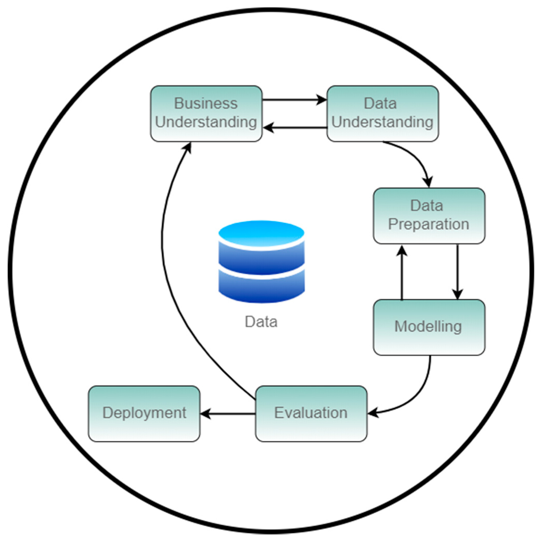
CRISP-DM model, represented on
Figure 1, is a hierarchical and cyclic process that breaks data mining process into the following phases (resume description) [
28,
29]:
Business Understanding: Determination of the goal.
Data Understanding: Become familiar with data and identify data quality issues.
Data Preparation: Also known as pre-processing and will have as output the final dataset.
Modeling: where a model that represents the existing knowledge it’s built through the use of several techniques. The model can be calibrated in a way to achieve a more accurate prediction of the target value defined as the goal on the 1st phase.
Evaluation: Evaluate the model performance and utility. This moment defines if a new CRISP-DM iteration will be needed or if to continue to the final phase.
Deployment: Deployment of the solution.
4. Work Methodology Proposed
4.1. Business Understanding
The main goal for this study is to contribute to a better growth assessment creating a new method to forecast a child’s height when they are an adult, also known as the target height. The model output will be personalized to the child (person-centric) and is expected to deliver a more accurate prediction when compared with the existing methods, already described in the previous chapters.
We began search for a “better” tool that provided a way to compare, for instance, a metric. We extensively researched this subject and found several methods for measure/comparing models’ performance, such as: Accuracy, confusion matrix, and several associate measures such as sensitivity, specificity, precision, recall or f-measure (very useful when facing classification problems with imbalanced classes), MSE—mean square error, ROC—Receiver Operating Characteristic Curve, AUC—area under the roc curve, RMSE—root mean squared error, MAE—mean absolute error, R²—R Squared, Log-loss, Cohen’s kappa, Sum squared error, Silhouette coefficient, Euclidean distance, or Manhattan distance [
30,
31,
32,
33].
The several methods/measures present different approaches for different problems (regression, classification, and clustering) with advantages and drawbacks. In this paper we will not describe or proceed with an extensive analysis on this subject, since other works, for instance, the ones mentioned as references, have already provided excellent analysis. Accuracy is a simple method (easy to compute and low complexity) able to discriminate and select the best (optimal) solution. It has limitations when dealing with classes and can result in sub-optimal solutions when classes are not balanced.
Our problem is not a classification problem, but a regression problem, and our goal is to provide better performance on our predictions. Considering our challenge characteristics, we believe the measure that best suits our goal is accuracy.
The performance results for the state-of-the-art height prediction when adult models were measured are presented in
Table 1. The best accuracy is obtained by the Mid-Parental Method which presents an accuracy of 59.53%.
4.2. Data Understanding
For the proposed study, was decided to use a dataset based on the famous study 1885 of Francis Galton (an English statistician that founded concepts such as correlation, quartile, percentile and regression) that was used to analyse the relations between child’s heights when adult to their parent’s heights.
The dataset is based on the observation of 928 children and the corresponding parents (205 pairs), where several variables have been recorded, such as father and mother height or child gender and adult height [
34].
Galton’s study made an important contribution in understanding multi-variable relationships and introduced the concept of regression analysis. It has proved that parents’ height were two Gaussian distributions (also known as normal), one for the mother and one for the father, that, when joined together, could be described as bivariate normal. It also has proved that adult children’s height could be described by a Gaussian distribution [
35].
The dataset used to this experiment is composed of 898 cases and the measuring unit is the inch. The dataset file includes the following information:
Family: Family identification, one for each family.
Father: Father’s height (in inches).
Mother: Mother’s height (in inches)
Sex: Child’s gender: F or M.
Height: the child’s height as an adult (in inches).
Nkids: the number of adult children in the family, or, at least, the number whose heights Galton recorded.
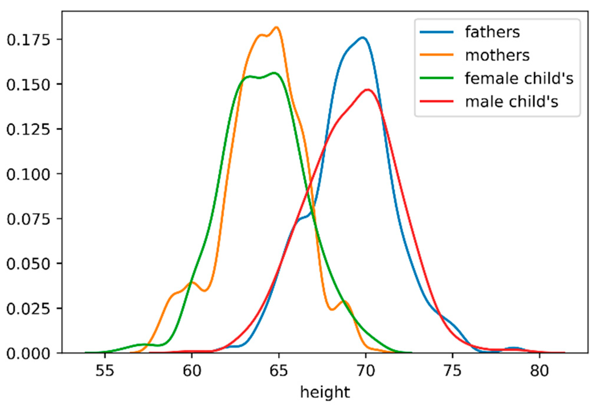
Figure 2 plots the distribution of heights on mother, fathers, child’s (regardless of gender), female child’s and male child’s. The horizontal axis represents the height, in inches, and on the vertical axis we can find the distribution density or another way the probability of a given value on the horizontal axis.
Analyzing the graphic provides the following conclusions:
Childs gender it’s a feature with high impact on height;
All “segments” heights (mothers, fathers, child’s, female child’s and male child’s) correspond to Gaussian distributions;
Female child’s and mother’s height distributions are similar. The same happens with the male child’s and parent’s heights.
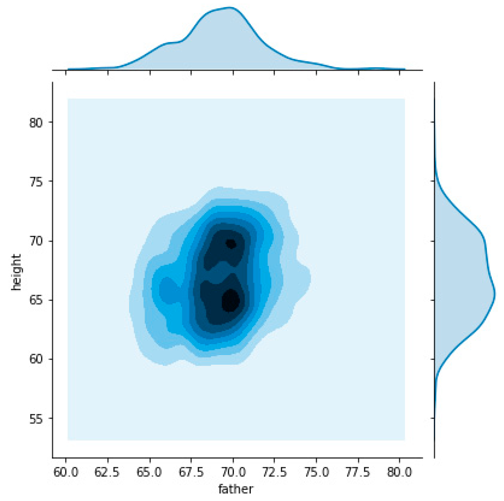
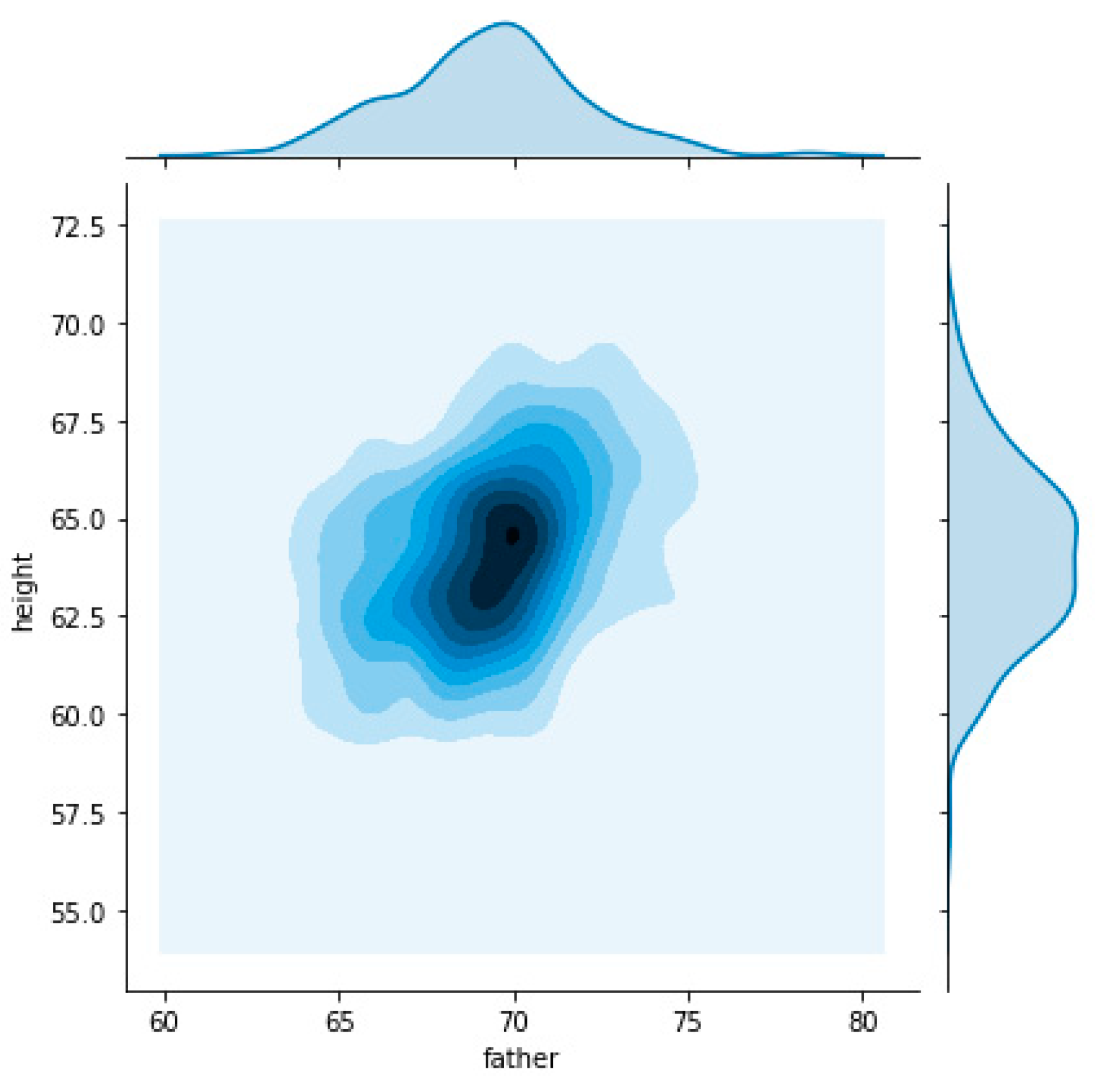
The following charts allow visualizing the relation between father’s heights, represented on the horizontal axis, and child’s heights on the vertical axis. On the first chart (
Figure 3) we used all dataset which made it possible to understand that the relation had two nuclei. This means that there are two “focus” on the relationship between father’s and child’s heights.
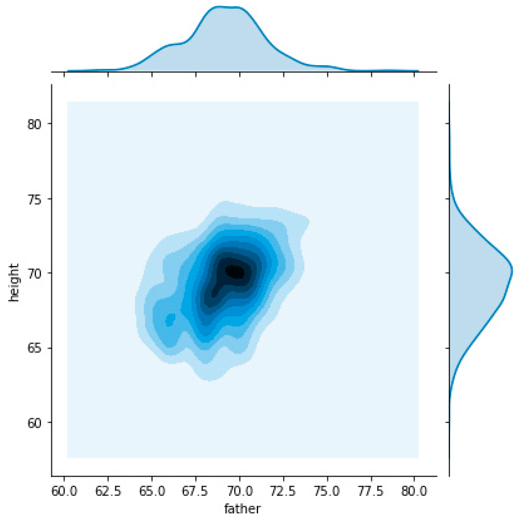
To understand these two different densities, we decide to split the dataset on male and female child’s what can be observed in
Figure 4 and
Figure 5, respectively.
Figure 4 and
Figure 5 clearly identity a relation of father’s height with child’s height that is different when considering child’s gender. For the same father height a child will be taller when male and shorter when female.
The same exercise was made using the mother’s height (rather than father’s) and we obtain similar shapes but show different influence dimensions. This analysis outputs a high degree of influence caused by the child’s gender as well as different influences from mother and father.
Understanding the influence on child height were different on father and mother we have performed a correlation analysis using person correlation measure.
Several approaches were implemented, such as analyzing children’s height by gender or parents, according to height distribution quarters. The results can be found in
Table 2.
Based on the obtained results we considered the following conclusions:
Parent’s height correlation with the child’s height differs between different child’s genders. This is evident for example when considering (all) father influence on female (0.459) and male (0.391) children. We observe a bigger influence on females.
Father height and mother height have different weights/influences on the child’s height. This can be observed for example on females’ child’s height correlated with father height (0.495) and mother height (0.314).
The parent’s height influence on child’s height it’s not constant, it varies among the height range.
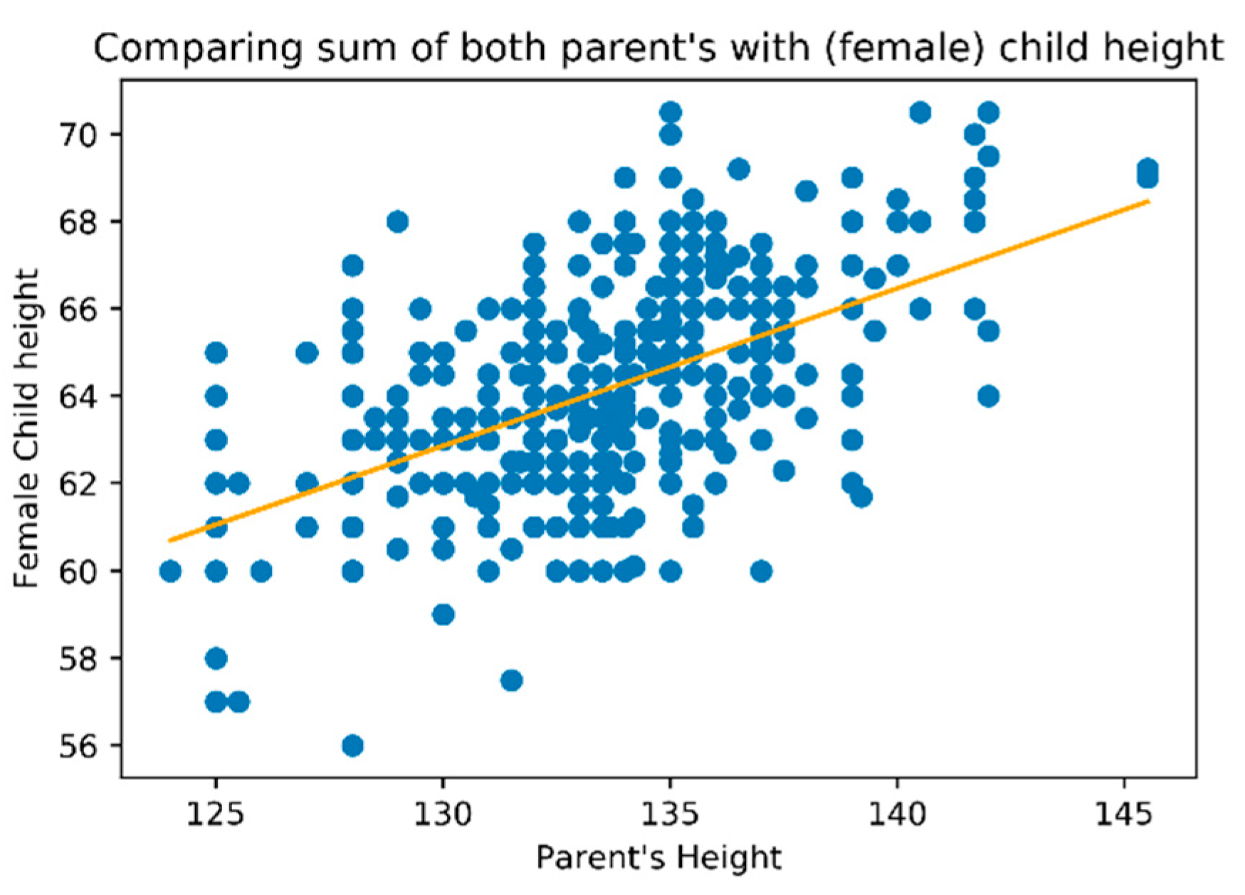
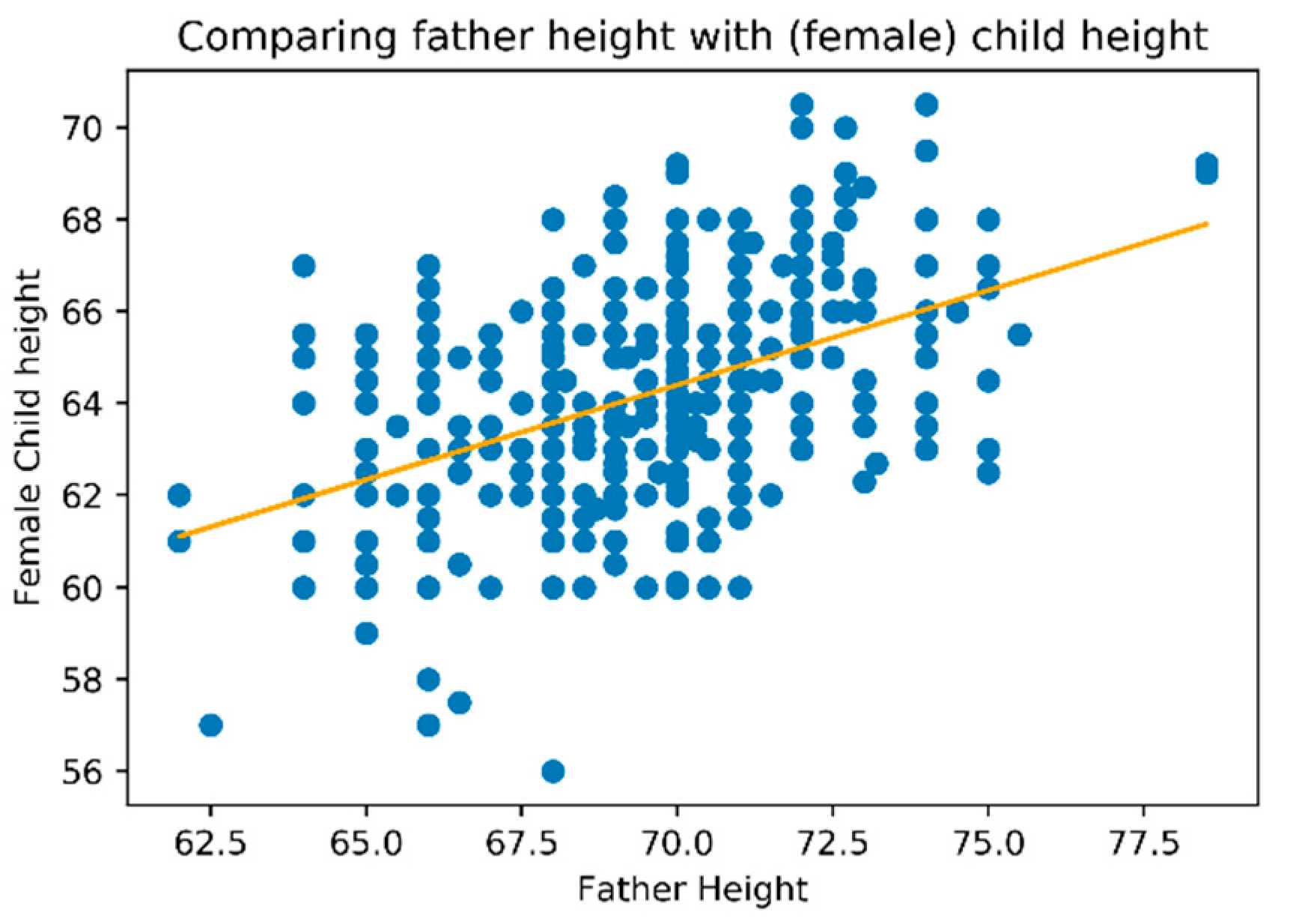
Based on the study dataset, a linear regression analysis was performed. We have taken several approaches, such as considering on the horizontal axis the sum of parent heights (
Figure 6), the mother height or father height individually and considering for vertical axis child’s height (regardless of gender), or considering the child’s gender (
Figure 7 for female gender).
We found a multilinear regression, where the child’s height dependended on the individual’s variable mother and father height. We also observed a high variance on the relations as it could easily be observed on the plots.
This phase also includes verifying the dataset for incomplete or missing data, errors, duplicates or other data issues. In
Table 3, it is possible to observe one of the tools used in our verification for checking information, such as the number of rows, that every row has values to every feature, or number of unique values for each feature.
There was no need for data cleaning or other tasks on the dataset. This was expected, since our dataset was previously used for other scientific purposes.
4.3. Data Preparation
The data preparation phase includes several tasks to achieve the final dataset to process, including feature selection, which is crucial to improving the models’ outcomes.
Feature selection can be performed using several techniques. These techniques can be segmented, a first step, supervised, unsupervised, and semi-supervised approaches. Inside the supervised segment, the category applied to our case, we can find different categories namely filter methods, wrapper methods, embedded methods, among others. Example of feature selection methods that fit these categories, include information gain, Relief, Fisher score, gain ratio, and Gini ind47ex [
36,
37,
38].
According to previous data analysis, the “family” feature defines the family to which the child belongs. The machine learning models can use the “family” feature to extract the brothers and sister heights when adults use this information to forecast their child’s height. In our scenario we did not want to use brothers’ and sisters’ heights, since in real cases, they are unlikely to be adults yet, and consequently we will not have this information. Therefore, we decided to exclude the family column from the dataset and eliminate family relations.
We have also excluded the “nkids” feature which refers to the number of brothers of an individual, since machine learning can also use this information. This information is not valid since, for instance, at the first brother born there is no information about how many brothers he will have in the future.
Considering feature selection, we also analysed the remaining features. Through the analysis performed in the previous chapter, we can verify that all of them seem to present a degree of influence on our prediction goal, the target height. Also, the algorithms that will be used on this study wrap feature selections techniques and those can address feature selection automatically. Considering these facts, we have decided to include all the remaining features in the modelling phase.
Finally, the gender feature was converted into a binary feature defining whether the child “is male?” so it can be used on the generality of machine learning models.
For applying machine learning supervised methods is necessary to divide the entire dataset on training and test sets. Usually a ratio of 80/20 or 70/30 is applied. We decided to use the first option. Once divided it’s important to assure that both (sub) datasets maintain the original dataset shape, which was assured as it can be observed in
Table 4 and
Table 5.
4.4. Modelling
To resolve the challenge, there was the need to choose which machine learning “tools” to use. For this study the criteria adopted was to choose the most popular machine learning algorithms, namely: Linear regression, SVR—Support Vector Regression (several kernels), Lasso, Elastic Net, Ridge Regression, K-Neighbors Regression, Bayesian Regression, AdaBoost Regression, SGD—Stochastic Gradient Descent Regression, Decision Tree Regression, XGB—Extreme Gradient Boosting Regression and LGBM—Light Gradient Boosting Machine Regression [
39,
40].
To pursue our goals, we start by applying all the previously described algorithms to our dataset, according to the partition described in the previous chapter.
For this study was used, as a development environment, Jupyter notebooks with Python 3.6 and the algorithms libraries Sklearn, XGBoost and Lightgbm.
Regarding the algorithm’s “configuration”, we have decided to start our modelling phase using the default (hyper) parameters which are defined by the libraries used on the study, mention above. The results obtained can be visualized in
Table 6.
Using this approach, we have achieved the goals outlined for the study, and several algorithms (such as SVR Linear, Ridge, Bayesian or Linear regression) were able to overcome the accuracy in the state-of-the-art models. Most of these algorithms achieved a small improvement, but XGB and LightGBM achieved a considerable improvement.
Based on the present approach, SVR Poly and SGD were difficult to converge and were not able to produce a valid output.
Although, the goals of the study, forecasting target height, and where possible, overcome the existing models, Horace Grey and Mid Parental method accuracy were achieved. It would be important to achieve the best accuracy possible, as the output is a valuable contribution to the growth assessment.
When using machine learning algorithms, it is possible to improve results using techniques like scaling and hyper-parameters tuning.
Regarding the scaling technique, our study has tried several approaches, namely techniques, such as StandardScaler, MinMaxScaler, MaxAbsScaler, RobustScaler and Scale. The best results were obtained with the MaxAbsScaler, which rescales data in a way that all feature values are in the range [0, 1].
Table 7 highlights the technique impact obtain on accuracy (column impact) when using MaxAbsScaler. The value “No change” includes very small challenges, mainly justified by the algorithms common variations.
Although, this technique improved the accuracy of some algorithms, an improvement was not made on the height prediction parameter.
Note, in this case, SVR Poly and SGD were able to converge and present a valid output, as the new scale overcomes the previous verified convergence issue with these two algorithms.
For hyperparameters tuning we considered two possible strategies: Grid search and Random Search. As Grid search requires a lot of resources and time to compute all possible algorithms and parameter dimensional space and those that adopted the random search strategy performed several iterations.
The applicability of this technique to the study dataset can be observed in
Table 8.
Hyper-parameter tuning has improved the accuracy of many algorithms, and most importantly, has achieved progress on the study goal, increasing children’s “target” height prediction accuracy.
Besides the importance of the performance output, it is also important to compare the complexities and costs regarding the algorithm’s applicability. We have decided to perform an analysis of the computation resources consumption required for each of the methods used above.
Since CPU consumption can present some variability, we decided to analyse CPU time mean and standard deviation by considering 1000 executions (
Table 9).
The computer supporting this study has the following characteristics:
Processor: Intel Core i7-3770 3.40GHz.
RAM: 8 GB.
Operating System: Windows 10, 64 bits, x64-based processor.
4.5. Evaluation
Through the output of the data mining process, we have obtainead several models that can forecast the child “target” height. Ten of those models have overcome the results obtained on the state-of-the-art reference model, Mid-Parental Method, and two of the models produced, XGB and LightGBM, with significant improvements. These two models have achieved the second goal defined in the business understating phase, improving the existing prediction accuracy.
Considering these results, it was possible to proceed to the next phase.
Regarding the computation resources consumption between different methods, we can verify that memory consumption presents a low variance (15%) with a minimum of 140 Mb and a maximum of 163 Mb. In our option, there was not a significant difference, even when dealing with large files, considering the availability of resources nowadays.
We can divide algorithms into four classes based on CPU time. The algorithms on the milliseconds range (i.e., Linear, SGD or KNeighbors), those on the tens of milliseconds range (i.e., AdaBoost or 26.6 ms), the class for the hundreds of milliseconds (i.e., SVR RBF or LightGBM), and finally the SVR Poly on the long-time processing class.
The CPU consumption is directly proportional to the algorithm’s complexity and it was expected to have a low processing consumption for a “simple” linear regression and bigger processing needs for support vector regressions. Remembering that linear regression method builds a linear equation (i.e., y = β0 + β1 × 1) that fits the best linear relationship between a set of input data to predict the output value, while SVR algorithms try to fit data using a hyper-plane where the support vectors threshold can assume different shapes (including nonlinear). These can vary according to the kernel defined as parameter [
41,
42].
Focusing on the algorithms that present the best improvements, XGB and LightGBM, we can observe a huge difference on the CPU consumption, where the last requests quadruple the time consumed by the first one.
Both algorithms are gradient boosted tree-based ensemble methods. XGB grows trees horizontally, as most of the tree base algorithms, while LightGBM grows tree vertically. That means that LightGBM grows from the leaf with greater loss (leaf-wise), while the other considers the level (level wise), what can reduce loss and result in better accuracy [
43,
44,
45].
LightGBM was developed after XGB and uses a novel sampling method called Gradient-based One-Side Sampling. It was developed with the purposes of achieving faster training, lower memory needs and better accuracy. Our results can confirm the accuracy overcome but we observe the inverse for the resources consumption. That can easily be explained as LightGBM was developed for large datasets, which was not the case in our study.
4.6. Deployment
After achieving the goals defined in this study, it is important to deliver an easy way for clinical professionals, particularly undertaking growth assessments, to benefit from this evolution. For that we have developed a basic interface (
Figure 8), connected by a web service to the model, that allows us to quickly introduce the inputs and generate the output prediction. This interface, model and service can be easily deployed to an existing IT infrastructure on hospitals, clinics, or other care facilities.
5. Results
In this study, we used several machine learning algorithms as a way to forecast a child’s height prediction when they turn into adults and we have also been successful in improving accuracy when compared with the currently existing models.
The models that presented the best accuracy were XGB and mainly LightGBM with considerable improvements when compared with the best-known existing model, the Mid-Parental method.
It is important to understand how LightGBM accuracy has been able to surpass the accuracy of the Mid-Parental method (the best model on state-of-the-art). Also, we believe that understanding the fundamentals of the prediction will make the model outputs more trustworthy for its users.
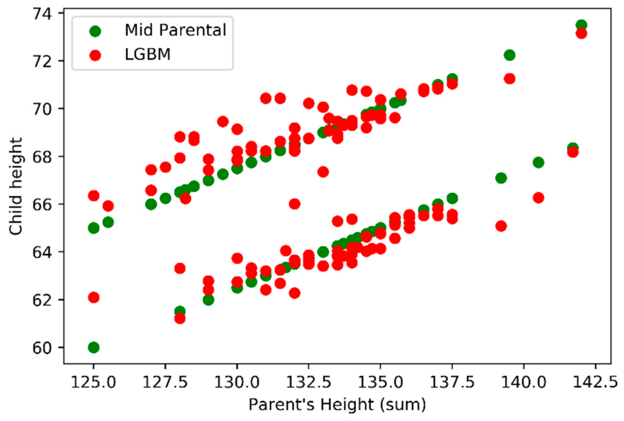
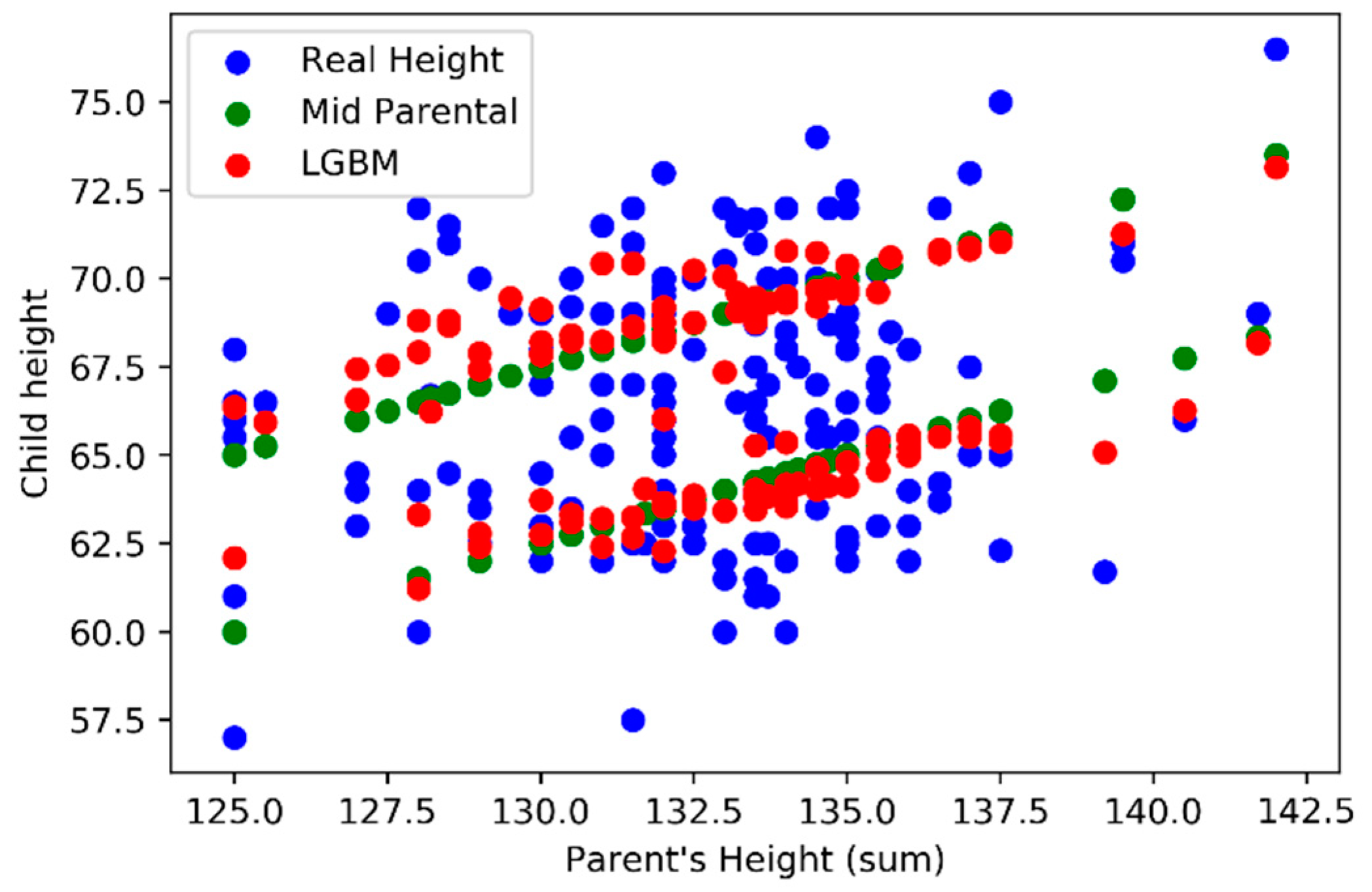
In analyzing the model outputs, we first decide to compare the outputs (vertical axis) against the sum of parents’ height (horizontal axis) using
Figure 9 where we can find LightGBM (red) and Mid-Parental methods (green) results. In
Figure 10 we also add the real values for the child height (blue).
In the previous figures (
Figure 9 and
Figure 10), was possible to verify that the Mid-Parental predicts the same child height, for the same gender, when considering the same parent’s height sum, while LightGBM model presents variations. When comparing both models LightGBM and Mid-Parental outputs with the real values it’s possible to understand that the first model is able to achieve predictions that are closer to the real values.
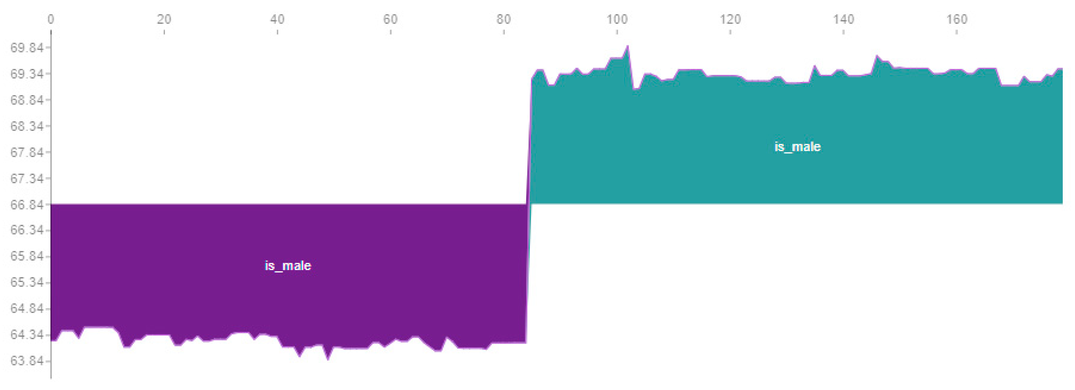
Focusing on gender influence on predictions, we verify that both models (LightGBM and Mid-Parental) were able to influence of gender the child height prediction.
The Mid-Parental considers a constant difference of 5 inches between male and female children. In
Figure 9, we can easily observe two parallel green lines formed by several green points, one for each gender, with a 5 inches difference.
Figure 11 shows the influence of gender on LightGBM in the dataset. The cadet blue colour presents male child’s (variable is_male = true) and dark orchid colour corresponds to female child’s (variable is_male = false). The influence of gender it’s not a constant of 5 inches, but otherwise its centre around 5 inches presents some small variability. The variability is about 0.5 inches on female (dark orchid area) and 0.7 on male (cadet blue area). The variability is not related to any trend on child height, but instead with the parents’ individual heights influence.
Previously, in the data exploration and visualization chapter, we verified that the influence of mother and father is different for different genders and for different mother and father heights. In
Figure 9, Observing figure 9 we can verify that our model (LightGBM) it’s able to capture and embed that variations that are not linear and where same parents’ heights produce different outputs.
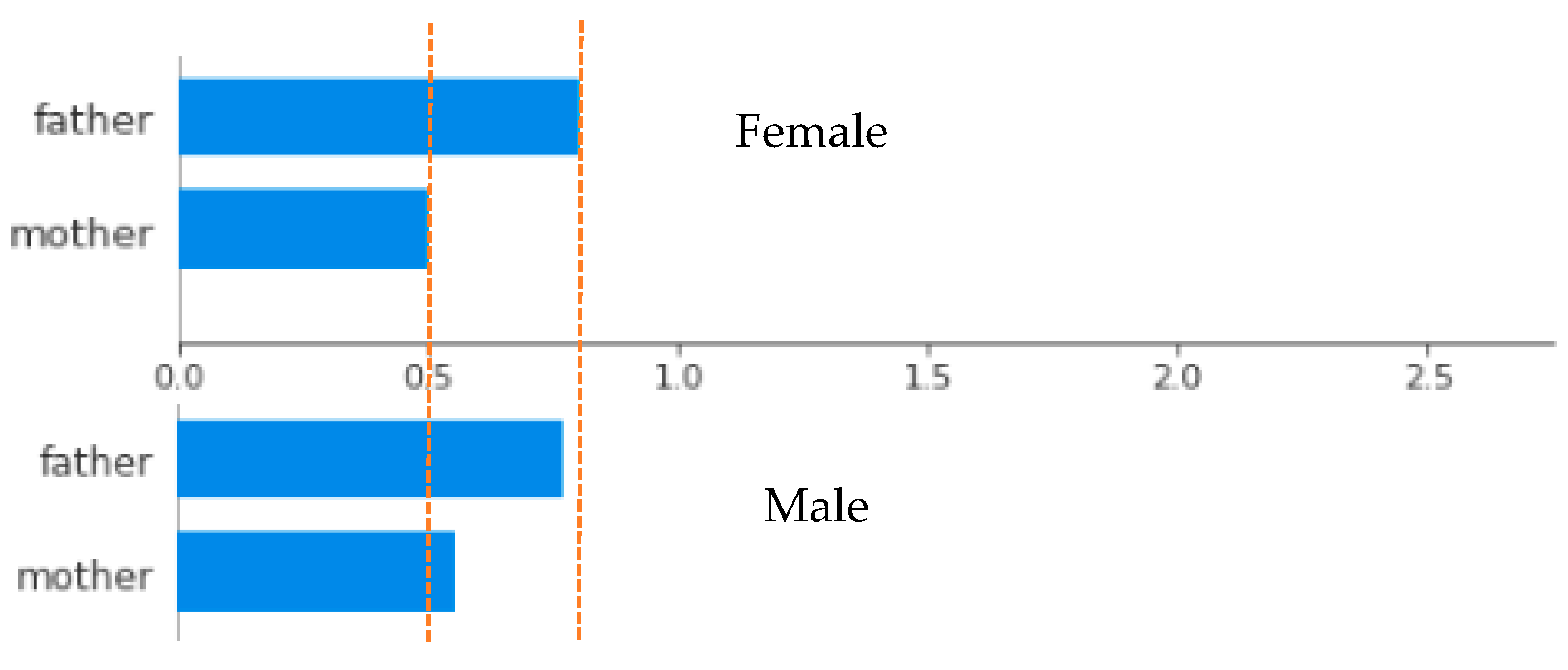
We have verified average fathers’ and mothers’ heights’ influence our model, according to children’s genders, as presented in
Figure 12. Importantly, fathers’ and mothers’ heights influence is different for different children’s genders. This fact confirms the results obtained on data exploration and visualization phase where we found, for instance, that the correlation of father height and female children was 0.459 and 0.391 for male children.
In
Figure 12, it is possible to observe the average influence of parent’s height. In
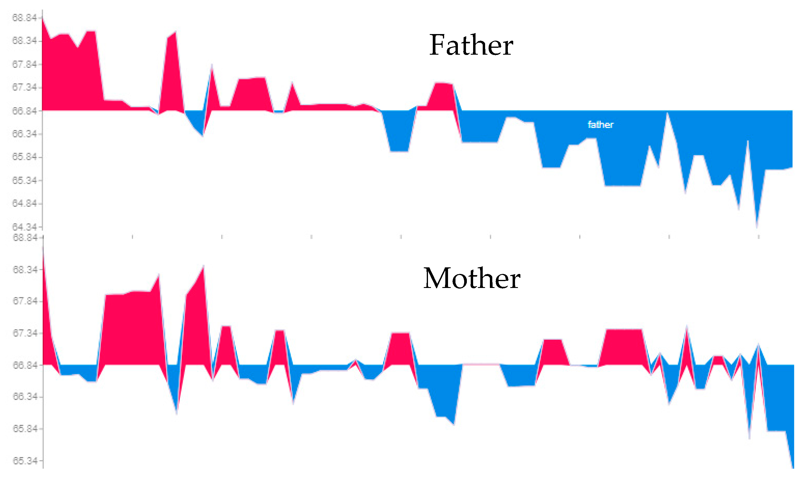
Figure 13, we observe the detail influence of mother and father height in the dataset records for a female child.
The graphic below represents all female children’s order from tallest to lowest. The red colour represents a positive influence and the blue colour a negative influence on the child’s height.
The most important fact to extract from the previous figure is that parents’ height influences their children’s height differently. The tallest female child, above the mean, mainly had a positive influence of fathers height, while the same is not true for mothers’ height, where we can see a lot of fluctuations.
By observing the oscillations, it is possible to see that the relationship is not linear, as defined by the Mid-Parental method, and that presents variance, mainly on the mother case. This variance was already observed in the data analysis phase, where we observed that the correlation between mother and female children have fluctuations.
Following the figure above (
Figure 13) we can verify that our model is able to incorporate the different influences of the parent’s heights on different situations. This leads to a model with better accuracy.
For the evaluation described above, we have used some resources from SHAP library, including some graphics generated by the tool. SHAP (SHapley Additive exPlanations) is a framework that combines features contributions and game theory to explain the machine learning predictions [
46,
47].
6. Conclusions
In our study, we assessed the ability to predict children’s height when they became adults, and we challenges ourselves to overcome the existing predictive models using machine learning techniques. Based on the developed work, our research group was able to find better approaches to forecast children’s height when they become adults. For most of the approaches, the improvements were minor but with the XGB and LightGBM algorithms were possible for achieving a considerable improvement on accuracy.
By analyzing the LightGBM model, we understood that our model was able to incorporate the different degree of influence of fathers’ and mothers’ heights in different stages, and on different children’s genders, what has contributed to improving the results obtained when compared with the previously existing models (Horace Grey and Mid-Parental method).
At the end of the study, we found that a step forward toward more personalized medicine, creating a new “tool” where growth assessments can be made using as reference the “real” potential growth for analysis in children.
The final model still has some variation when compared to real values. We believe it can be reduced by adding other signification variables to the model, such as grandparent’s height, existing pathologies, economical level and alimentation access/quality. This will be probably approached in future work.
In future work, we would like to develop three new studies:
Use the procedures defined in this article for a current population, using a bigger dataset. Contact with Portuguese public institutions/services is being made to explore the current Portuguese height records.
Develop a new approach where the height of a child is forecast from birth to adulthood, monitoring the full development by year, and where data from previous years will probably take prominence.
Use the methodology defined for this experience using a dataset with more features. We would like to add to the existing features variables, such as grandparent’s height, existing pathologies, economical level and alimentation access/quality. We are already developing contacts with Geração XXI project (Portugal) that has created a cohort study with a considerable number of child’s (about 8000), that can help to deepen this study.
We believe that other features can reduce the variability on the model, and consequently increase accuracy.


