Automatic Tuning of High Piano Tones

Abstract

Piano tuning is known to be difficult because the stiffness of piano strings causes the tones produced to be inharmonic. Aural tuning is time consuming and requires the help of a professional. This motivates the question of whether this process can be automated. Attempts at automatic tuning are usually assessed by comparing the Railsback curve of the results with the curve of a professional tuner. In this paper we determine a simple and reliable rule for tuning the high tones of a piano with the help of a listening test. This rule consists of matching the two tones in an octave interval so that the first partial frequency of the upper tone becomes exactly the same as the second partial frequency of the lower tone. This rule was rated best among four tuning rules that were compared in the test. The results found are explained using a beat-based analysis, and are consistent with some previous studies. They are also tested against the existing method of using Railsback curves, and it is shown that comparison using Railsback curves is an unreliable method of assessing different tunings. The findings from this paper can be used to create a complete automatic tuner that could make the process of piano tuning quick and inexpensive.

1. Introduction

Pianos cannot be tuned like other string instruments. The strings of a piano have a significant stiffness which causes the tones produced to be inharmonic [1,2,3,4]. This means that the partials above the fundamental have a frequency which is slightly higher than the expected integral multiple of the fundamental. In a piano, due to the shifted frequency of the partials, the frequency ratio of known intervals is changed. Every piano is different, and the inharmonicity varies from string to string. Thus, tuning is not as simple as tuning every string to a known fundamental frequency, as is the case with most other string instruments. Professional tuners listen to the tones produced by each key of a piano, and make them in tune with an already tuned tone, at some interval from it, based on their experience. The ultimate goal of this study is to produce results as good as those of a professional tuner with just a computer. This has the potential to lead to an automatic piano tuner providing a cheaper and faster alternative to piano tuning by a professional.

Previous work has been carried out to find a method to automatically tune the piano. Most approaches involve matching the frequency of specific partials for two tones in an interval [3,5,6]. One approach involved calculating the sensory dissonances between tones and minimizing them [4]. Another unique approach was to minimize the Shannon entropy of all tones in a piano [7]. All these seem to produce quite good results. However, the results have not been backed with formal listening tests; and since it is ultimately humans who decide the tuning process and what should be a “good” tuning, it should be them who decide how well these tuning methods do.

In order to create an automatic tuner, it is important to first identify what a “good” tuning is. We can say that one tuning is better than another if it is preferred by listeners. Based on the fact that professional tuners primarily use beating rates to tune [8], we can hypothesize that a good tuning would be one with minimum beating for commonly used intervals. Previous papers seem to consider a good tuning to be one that is exactly the same as a professional tuner. However, every tuner has their own style of tuning, and there is no one perfect tuning curve. Rather, there are many possible curves which sound acceptable [2]. It is shown later in this paper that the comparison of two different tuning rules on two differently tuned pianos gives different results.

Most previous studies judge the success of their proposed methods by comparing the deviation of the fundamental frequency of the automatically tuned tones from the fundamental frequency of the tones tuned by a professional tuner. As mentioned above, different tuners have different tuning curves. Combined with the fact that almost every approach has been tested on a single tuning of a single piano, the results do not provide as much insight on the method proposed as it may seem initially. While trying to obtain a tuning accuracy that will be able to tune even concert pianos in the future, it is important to come up with some other means of judging the success of a tuning method. This means of assessment should not be biased towards any specific piano tuning. In this paper, one such method of analysis is proposed, which is based on the beating rates of tones.

Piano tuning is generally conducted in three segments starting with the reference octave (usually from F3 to F4), followed by the tones above the reference octave, and finally tones below the reference octave [8]. The best tuning for high piano tones involves adjusting octaves so that partials of upper and lower tones match as closely as possible. One way to do this is to make the first partial frequency of the upper tone exactly the same as the second partial frequency of the lower tone. These two partials are the first partials of each tone that would overlap (i.e., be of the same frequency) when tuning harmonic tones, and so we call them the first set of matching partials. Another way to do this is to make the second set of matching partials overlap exactly. We may also find a middle ground between the two. A listening test aims to identify which of these methods people think sound the best. The results are compared with a beating analysis and the reliability of using it as a test of success is judged. With the results of the listening test, this analysis confirms that listeners prefer octaves where the beating is minimum. Thus, the first outcome of this paper is a simple rule to tune high piano tones, based on a conducted listening test. The second outcome is a method of measuring beating rates, which is proposed as an alternative method to test the success of a tuning algorithm.

This paper is organized as follows. Section 2 explains the preparations needed for the listening test, including recording of piano tones, selection of the tuning rules, and the generation of test signals. Section 3 describes the design of the listening test. Section 4 presents the listening test results. Section 5 proposes a signal analysis method to explain the audibility of mistuning in octaves, compares the various tuning rules in the light of signal analysis, and discusses why comparison using Railsback curves may not be a reliable method to compare different tunings. Section 6 concludes.

2. Preparations for Listening Test

2.1. Piano Tones

One of the major problems faced previously with recording piano tones was getting each key to be played with exactly the same weight, in order to have a set of tones with equal volume. This is required to ensure that the results are independent of the changes in the spectrum of a tone due to change in the volume with which it is played. Thus the Disklavier, which accepts MIDI input, was chosen so that the loudness could be controlled very accurately, as well as the length of each recorded tone. The microphone used for the recording was the DPA IMK-SC4061 Instrument Mic Kit. It was chosen due to its relatively flat frequency response in the required frequency range. It was connected to the computer with the MOTU UltraLite mk3 interface, and the sampling frequency was set to 44.1 kHz.

The tones used in the listening test were recorded on a Yamaha Disklavier at the Music Center, Helsinki, Finland. The piano had been tuned by a professional tuner a few hours prior to the recording, and had not been played until the recording. This is important as the strings get detuned with use. Thus we can safely say the recordings showed what a professionally tuned piano should sound like.

The Disklavier was placed in the center of a closed room which was well sealed acoustically. Before recording, the left and right strings were damped for every key using a tuning ribbon, for all keys with three strings. Consequently, the recordings were done for the middle string. For those keys with two strings, the right string was damped with a tuning wedge and the left string was recorded. The tones were recorded twice, once with the keys played loudly, and once softly. On later analysis, the loud tones were found to have a better signal-to-noise ratio, and thus they were used in the listening test and other simulations.

2.2. Rules Tested

Using the recordings obtained, different tunings were generated for notes above F4 (key #45), as the goal of this study was to focus on the tuning of high tones of the piano. The aim was to compare some simple rules on how to match the partials of the two tones in an octave. These rules were adapted from previous approaches [3,5,6]. The different rules tested for two tones an octave apart were as follows:

• Matching first partial (m1): the upper tone was modified such that the first partial of the upper tone overlapped exactly with the second partial of the lower tone, i.e., they had the same frequency.
• Matching second partial (m2): the second set of matching partials exactly overlapped, in a manner similar to the previous one.
• Geometric mean (GM): the geometric mean (GM) of the frequencies of the first two sets of matching partials were made to be equal. The GM of the second and fourth partial of the lower tone was calculated and the upper tone was modified such that the GM of the first and second partial was made equal to it.
• Matching third partial (m3): the third partial of the upper tone and the sixth partial of the lower tone were made to overlap. As the amplitudes of the partials drop off very quickly at high octaves, this rule was expected to be worse than the others. It was included as a low-quality anchor for the listeners, to define the worst performance in each trial.

For the listening test, samples were chosen primarily from the sixth and seventh octave. In the last octave (the eighth octave) the decay of such high tones is very quick and this makes it difficult to hear beating. According to a study conducted, it is difficult to identify beating cues for tones shorter than 1 to 2 s [9]. The same study also showed that identifying mistuning in very high frequencies is difficult [9]. This is why, often larger intervals like double and triple octaves are used to tune the highest octave [8].

Below the chosen range, in the octaves just above the reference octave, the results always seem to be pretty good. Deviations occur only in the higher octaves, and thus the two octaves just beyond the reference octave are not used in this listening test. The lowest tone used was F6, with a fundamental frequency of about 1.4 kHz, and the highest tone was D7, with a fundamental frequency of about 2.4 kHz. Eight different tones were chosen in this range.

2.3. Generation of Test Tones

Each sample used in the listening test was a superposition of the two tones an octave apart, tuned as described above. In the generation of the samples, the lower tone was taken as is and the frequency of the upper tone was modified to fit the rule mentioned. This modification was realized by scaling the signal using upsampling or downsampling, while maintaining the same sampling frequency. This works under the assumption that with the small frequency changes of at most 3% that are made in order to simulate tuning, the inharmonicity coefficient of the string does not change much.

The frequency of individual partials of a piano tone depends on the fundamental frequency $f_0$, inharmonicity coefficient (B), and partial number (n) according to the following formula [10]:

$$f_n=n{f}_0\sqrt{1+B{n}^2},$$

(1)

where

$$f_0=\frac{1}{2L}\sqrt{\frac{T}{m/L}}$$

(2)

and where m is the mass density of the string, L is the string length, and T is the string tension. Scaling the fundamental frequency linearly causes a linear scaling of each of the partials assuming a constant value of B. However, the value of B is inversely proportional to the string tension T, which is increased or decreased while tuning, to change the fundamental frequency $f_0$. We can use these two relations to find the effect of change in the inharmonicity coefficient ($\Delta B$) with the change in fundamental frequency ($\Delta f_0$). As we are dealing with very small changes in frequency, we can differentiate the two equations, and equate the results. The relation obtained is:

$$\frac{dB}{B}=-2\frac{d{f}_0}{f_0}$$

(3)

or

$$\frac{\Delta B}{B}=-2\frac{\Delta f_0}{f_0}.$$

(4)

Thus, we can conclude that a very small change in the fundamental frequency brings about a small change in inharmonicity. Thus the assumption stated before is satisfied and simple scaling can be an accurate simulation of the actual tuning of strings. In fact, this change in B is generally smaller than that observed in the B values of neighboring strings. For a frequency change of 3%, the B value varies by 6%. We checked from the data provided by Tuovinen et al. [6] that the change in B value between neighboring strings in the chosen range is between 5% and 18% for all pairs of strings except one, which has a change in B value of 2.6%.

Each individual tone was normalized to sound approximately equally loud, and the final superposition signals were also normalized to have approximately the same loudness. It was verified in an informal pilot test that none of the octave signals was softer than the others and that the two tones in each superposition signal were clearly audible and not softer than the tone with which it was added to. The length of the condition chosen was set to 170,000 samples or about 4 seconds, and the onset or attack was at about 1 second in each audio file.

3. Listening Test

The listening test was conducted using the WebMUSHRA software [11]. The test was a Multi Stimuli test, similar to MUSHRA. The conditions included a hidden anchor but no reference, because there is no ground truth in piano tuning. The reference button still appeared on the test page, but participants of the test were told not to use it. The participants rated the conditions using the vertical sliders, which were initially set to maximum (100) on each page. A screenshot of the test environment is shown in Figure 1. Audio files used in the listening test are available online at http://research.spa.aalto.fi/publications/papers/applsci-tuning/.

The test began with the instructions and volume setup, followed by a training page. It was not allowed to change the volume setting after the training. The training had some conditions that were ordered according to their beating rates from lowest to highest. These were not to be rated, and participants could listen to these in order to get an idea of what the different tunings of piano tones sounded like. The subjects were told that the test is about different tuning systems for octaves, but they were not instructed to listen to the beating. They had to figure out an evaluation strategy themselves. Following these were 18 trials where subjects had to rate the different samples, or conditions.

In each trial, subjects were presented with five conditions; the octave as tuned by the professional tuner, and by the four other rules described earlier. They were asked to rate the conditions based on their tuning from bad to excellent, on a scale of 0 to 100. The first two of these pages were for training, where participants were asked to rate the conditions, but these scores were not taken into account while extracting information from the results. The results of the remaining 16 trials were accounted for while analyzing the results. These contained samples from eight different octave intervals, repeated twice, and presented in a pseudorandom order.

It was thought that it is important in this listening test to include participants who are critical listeners, but not necessarily pianists or professional tuners, because the tuning should sound good to all listeners. Experience in playing a musical instrument and in listening tests was considered to be preferable. A total of 17 people were invited to take the listening test. Before the test it was decided that if any participant gave a full score for the rule m3 (the anchor) more than thrice, their results would be discarded. Based on this, one set of results had to be removed. Out of the remaining 16 participants, 15 reported having played some instrument. All 16 participants had a background in acoustics or audio signal processing, and had prior experience with listening tests.

4. Results

The results are shown with a 95% confidence interval (as per the ITU recommendation [12]) in Figure 2 and in

Table 1. Table showing the results of the listening test. The values of the mean and 95% confidence interval (CI) are given for each tuning rule. The best mean result is highlighted.

Tuning Rule	Mean	Lower CI	Upper CI
Professional tuning (n)	68.7	66.3	71.2
Geometric mean rule (GM)	65.9	63.3	68.4
Matching first partial (m1)	75.0	72.5	77.5
Matching second partial (m2)	61.6	58.7	64.4
Matching third partial (m3)	39.2	36.1	42.3

. It is seen clearly in Figure 2 that the rule that stands out is matching first partial (m1). The range of the rule m1 is higher than the rest, and does not overlap with the other ranges. It can be concluded that the listeners thought that the samples tuned using rule m1 were best tuned on average.

The results for each octave were also similarly plotted, and some of these are shown in Figure 3. It can be seen that the outcomes are not exactly the same for every octave. Although they follow a similar trend to the overall plot, two plots are significantly different. The plot for octave D6–D7 in Figure 3b does not have rule m1 with the best rating, as is the trend. This is possibly because it is harder to hear beats at higher octaves due to really fast decay [9].

The second octave with deviated results was A5–A6, in which it appears that every method has roughly equal scores on average, with overlapping confidence intervals, as shown in Figure 3a. This may be because of the increasing inharmonicity with frequency, which makes it possible to match multiple partials at once [13]. However, if we look at the results overall, we can see that rule m1 seems to be doing clearly best in most cases. In no octave has any other rule clearly gotten a better score. The professional tuning has gotten a higher average score than rule m1 in a few octaves, but is not clearly the best tuning for any single octave. Rule m3, the anchor, has clearly gotten the worst scores in all octaves, as expected. Figure 3c shows an example of a typical result for a single octave in which rule m1 gets the best rating and anchor m3 the worst one.

It is somewhat surprising that listeners did not in fact find the professional tuning to be the best tuning in every octave. This can be explained by the fact that tuners sometimes use additional tests, for example double octaves, for fine tuning the tone [8]. These tests are subjective, and used differently on different pianos and on different octaves. We can thus say that despite some variations in individual octaves, it appears that, on average, the octaves tuned using rule m1 have been perceived to be the best in tune by listeners.

The results of the listening test have also been used to substantiate the claims of beating rates being a better identifier of the quality of tuning than Railsback curves [1]. This is explained in further detail in the next section.

5. Beating Analysis

Harmonic tones can be tuned exactly by making sure the beats completely vanish (while tuning octaves). Due to the inharmonicity of its strings, it is impossible to achieve this zero-beat condition for piano tones. There exist different beating rates for different sets of partials, and we can expect that tuning piano tones would require the minimizing of some function of these rates. Professional piano tuners in fact do just this, and it is the primary basis for their tuning process [8]. This suggests that plotting the beating effects of the many pairs of partials might provide a good point of analysis. This method is especially suited for high tones as they have very few significant partials; beyond the third partial, every partial is of very low amplitude and can be neglected.

The first step was to separate the different partials. The two tones were superposed and three bandpass filters were used to isolate the required pairs of partials. The specifications of the bandpass filter depended on the fundamental frequency of the lower tone and the inharmonicities of both tones. A buffer of 10% of the distance between two partials was used. This resulted in three signals having a pair of partials, one from each tone. These partials are very close and each pair causes its own beating. The processing that follows was done on each of these signals.

Beating is essentially amplitude modulation, and so it is extracted by finding the envelope of the signal. The envelope of the signal was found using the help of Hilbert transform. The Hilbert transform is a linear function that shifts the phase of each Fourier component of the signal by 90 degrees in the frequency domain.

The spectrum of the envelope by itself gives quite erratic results, with a lot of noise in the low frequency region of the signal, which is where the rate of beating should be found. In order to counteract this, three extra operations were performed. First, the envelope of the signal was fit to a second-order exponential function in order to remove the decay of the tone. The second order exponential function was chosen because it provided clearer results, perhaps because of double decay [14]. The found exponential function could then be either subtracted from the original envelope signal, or it could divide this signal. Both methods have their advantages and disadvantages, but provide comparable results. This will be described in more detail in the next subsection.

The second operation done to improve the results was to use the detrend function, which brought the average of the signal to zero, thereby removing noise in the low frequencies of the spectrum, which had a peak at 0 Hz before using this function. The detrend function subtracts the mean or best fit of a function and thus removes the low frequency fluctuations in a signal.

The third alteration was made to the length of the signal. The signals were almost 4 s in length. However, the decay of the tones happen much quicker. Thus, the envelope was only used until the signal reached 2% of its maximum amplitude. In cases where the amplitude of the signal was so low that the noise in the channel was more than 2% of its maximum amplitude, a fixed numerical amplitude cutoff was provided based on the observed noise.

Finally, the signal was passed through a lowpass filter to remove unwanted high frequency noise. The maximum beating rate is about 15 Hz, and so the cutoff frequency of the lowpass filter was chosen to be 20 Hz. The FFT function (fast Fourier transform) was then used to calculate the signal spectrum. A rectangular window of size $2{}^2{}^0$ was used, with the signal padded with zeros on either end to attain that length. The absolute value of the signal was taken and converted to the dB scale before plotting it.

5.1. Results (Beating Analysis)

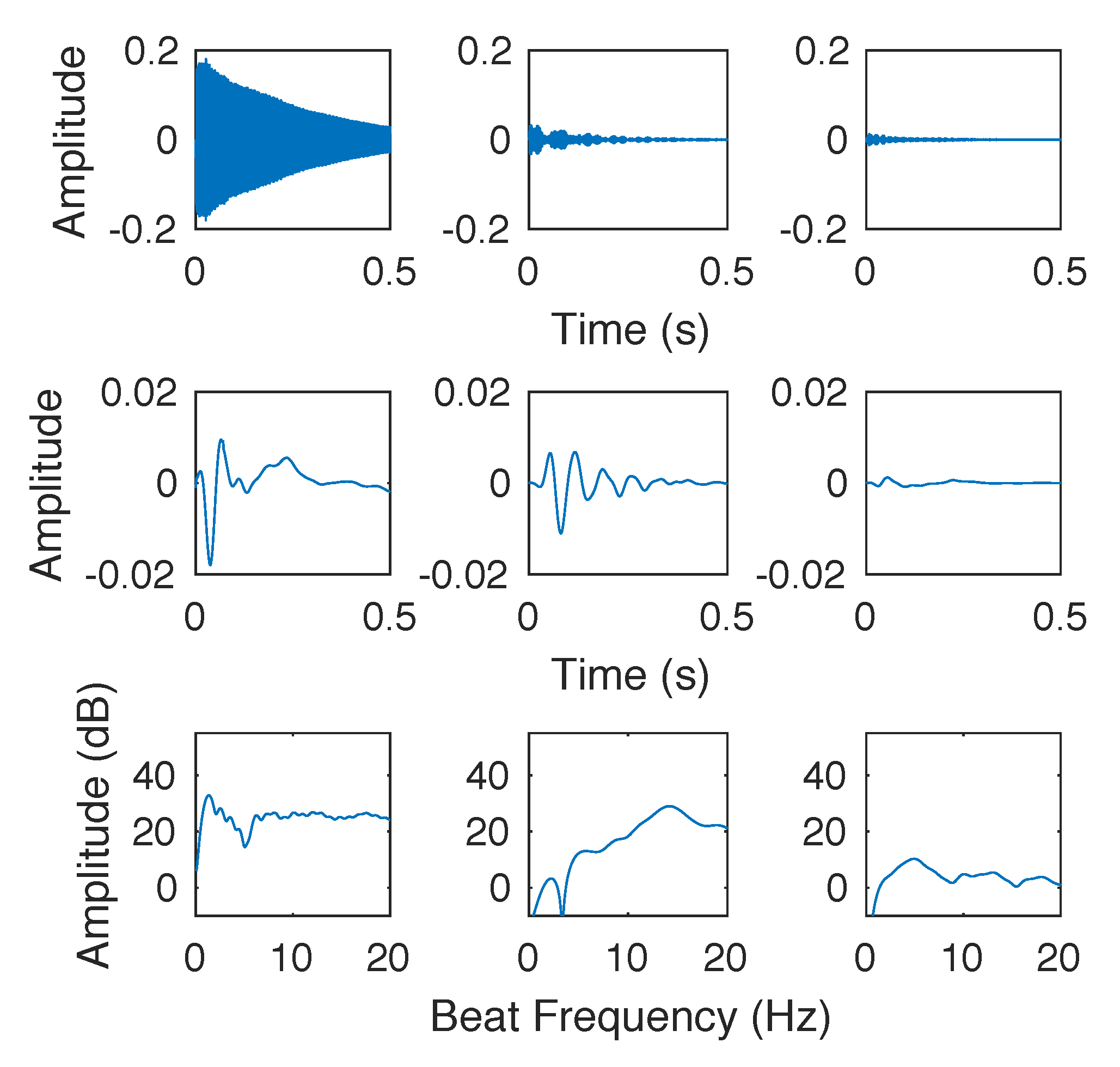
An example of the plots generated can be seen in Figure 4. Each column refers to a single partial. The top graphs show the time domain signal, the middle graphs are the envelope functions that have been processed. Finally, the bottom graphs show the spectrum of the envelope, which reveals the beat frequencies. The plots are made for two methods of processing the envelope: subtracting the decay function and dividing the decay function.

In the example in Figure 4, it can be seen that the envelope function post processing gives a good impression of the amplitude modulation in the original signal. Although the spectrum of this envelope does not have sharp peaks, the beating value can still be found as the global maxima in the plotted frequency range. For the first set of matching partials, it is about six beats per second, and for the second set it is about three beats per second. The third set of matching partials has a very noisy signal with no obvious beating rate. Thus the frequency spectrum is more or less flat. These results correspond to the quality of tuning, with smaller values for number of beats being the goal.

One slight problem with this approach is that the ideal envelope function is not a sine wave but a rectified sine wave. This is one reason why the peaks in the magnitude spectrum are not very sharp. Other windows were also tried, but it seems that rectangular window are the most appropriate for our requirements as they have the narrowest main lobe (sharpest spectrum), despite having relatively high amplitudes for the side lobes.

Another interesting result that was noticed was that, in general, the beat frequency increased linearly with the partial number of the higher tone being matched. This can be seen clearly in Figure 5. This result is expected as the frequency of the partial increases as the inharmonicity causes the partials to get farther apart. Despite this being the case, it is also seen that due to the increasing inharmonicity with key number, it is sometimes possible to match both the first and second set of partials almost exactly, which is in line with previous studies [13].

Although the beats were plotted for three sets of matching partials, this can be extended to include as many partials as required. It was noticed that for high tones, the beating of the third set of matching partials is very insignificant compared to the previous two. In a lot of cases, the amplitude of the signal corresponding to the third set of matching partials was so low that the ambient noise in the recording, which is actually very low, becomes significant in comparison. In these cases it is very difficult to plot the beating rate. However, it is also unnecessary because when the amplitude is so low, then the beating could not be heard either. Thus, analysis using the first two sets of matching partials is actually enough.

Although the results seem very promising, they are not perfect. In some cases, there are two peaks of almost the same height and so both must be considered. Secondly, the reason that the spectrum is plotted for the signal processed in two different ways is that in a few cases, one method seemed to provide better results, while in some others, the other method appeared to be better. However, both methods seem to provide the same maxima for most tones. Overall, dividing the envelope with the exponential function gives a better result. However, sometimes the amplitude of the envelope seems to grow with time as the exponential function does not fit perfectly. This creates an unrealistic result for the beating rate.

The algorithm suggested in this section is vital for many reasons. The first is that it provides an alternative method to judge the accuracy or quality of tuning. Professional tuners are trained to listen to beats and use them throughout the process of tuning. Thus, being able to find the rate of beating using a computer could enable an alternative method to test the accuracy of different tunings, and can be used for automatic tuning, where a professional is not available to do so. This is explained in more detail in the next section.

5.2. Comparing Different Tuning Rules

Since aural tuning relies so heavily on beats, it is possible to use this algorithm to create an automatic tuning process that follows the exact steps of a professional tuner. Although the plotting was done with an emphasis on high piano tones, it can be extended to other tones on the piano as well. It can be extended to different intervals and different number of partials. The tuning of the reference octave especially relies heavily on counting beats, and thus being able to plot the beating rates is a very valuable tool. Here are some results that were observed based on looking at the beating rates for various different tunings (see next section for the tunings):

• In order to obtain a good tuning, the beating effect from the first set of matching partials is most important; if that beating is reduced to zero, then the beating in the second set of matching partials might be insignificant. This is possible because the partial amplitude decreases very quickly with partial number for high tones. This is more applicable as you increase the key number.
• Overlapping the first set of matching partials always seems to minimize the beating rates best. This rule of tuning sometimes even does a better job than the professional tuner, who seems to have left some very prominent beating in the first set of matching partials.
• The rules of overlapping the second and third set of matching partials usually do not provide results as good as the other rules.
• The rule of geometric means has very unreliable results, sometimes having low beats, while at other times having significant beats in the first set of matching partials.

These observations match very well with the results of the listening test (cf. Figure 2), thus giving this method credibility as being a good measure of well-tuned octaves. The listening test also concluded that overall, matching the first partials provided the best results, sometimes even better than the professional tuner.

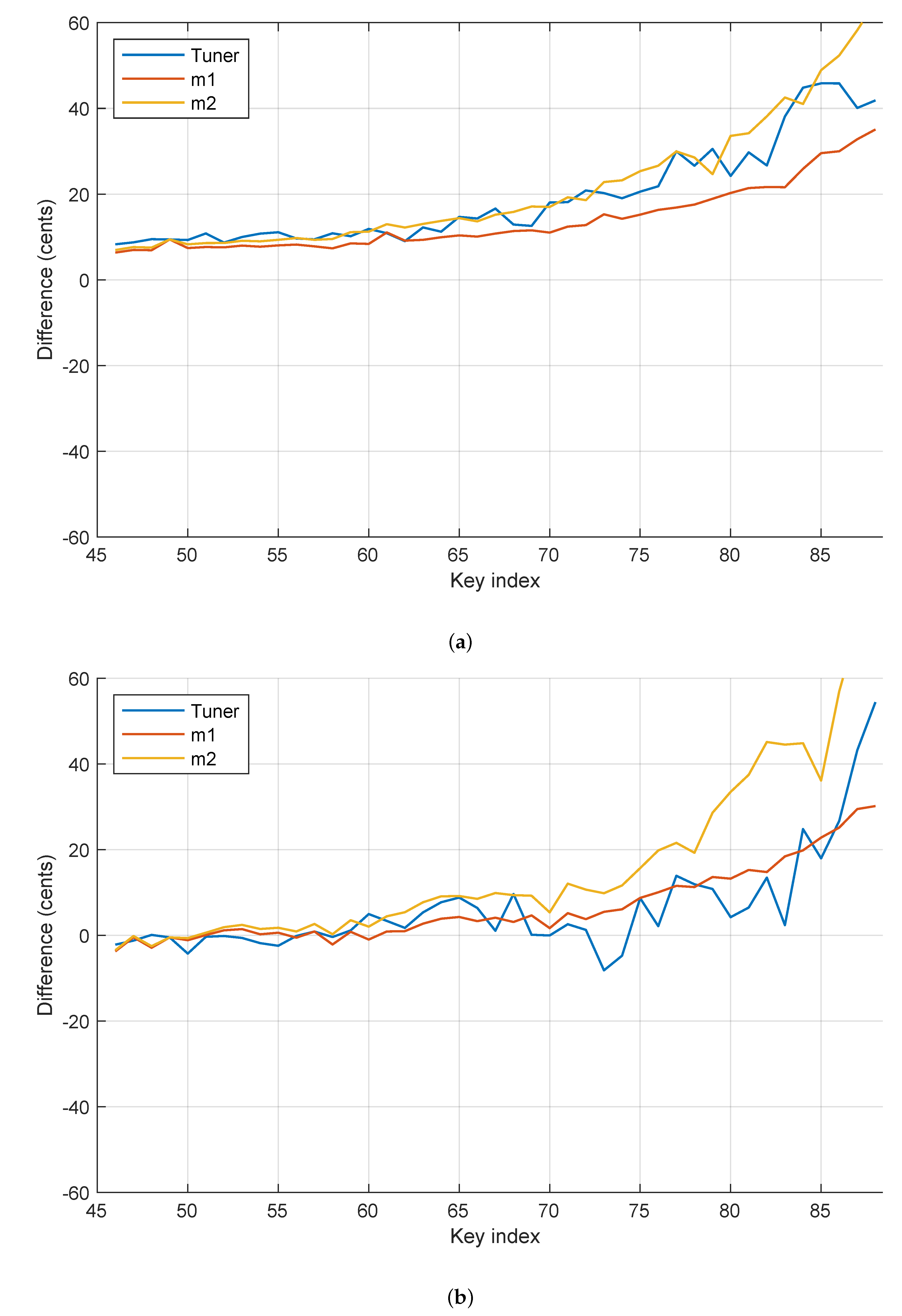
5.3. Comparison of Railsback Curves

The success of various automatic tuning algorithms have been determined by comparing different tuning curves. We propose that analyzing beats provides a better method for determining this success. In order to justify these claims, two octave tuning rules for tones above the reference octave have been chosen and tested on two sets of recordings from two different pianos tuned by different tuners. The comparison provides an insight about why Railsback curves are not meant to be used to compare the goodness of two different tunings.

The first set of tones used were recorded on a Yamaha Disklavier (refer to Section 2 for the details of the recording). The second set has been borrowed from Tuovinen et al. [6], who recorded them using a Yamaha grand piano. The first method chosen was to match the first set of matching partials (rule m1) and the second matched the second set of matching partials in each octave interval (rule m2). The Railsback curves for both rules of tuning have been plotted along with the professional tuning for each set of tones in Figure 6.

As can be seen in Figure 6, the curves obtained show contradicting results. It appears that in Figure 6a, tuning rule m2 fits better on the set 1 tones by comparing closeness to the tuner’s curve. However, the plot for set 2 tones in Figure 6b shows that the tuning rule m1 matches more closely with the professional tuning. As most papers have the results only on a single piano, they are not reliable if being tested by this method.

Another disadvantage of this method is the cumulative effect in errors, as piano strings are tuned by going up the keyboard step by step. For example, while tuning a tone in the seventh octave, there may be a small error. However, in the tuning curves the compound error is visible, for that tone, which consists of that small error, plus the error in the octaves before it, which were tuned previously. Using the distance of the tuning curve as a local measure of how well that portion of the piano is tuned is thus inaccurate.

We will now compare the different beating plots with the listening test results. Figure 7 and Figure 8 compare the beating plots of two tuning rules for the octave Bb5–Bb6. The first row in each figure depicts the temporal waveform representation of the signal. The second row shows the processed envelope function, and the final row shows the spectrum of the envelope.

It can be seen that in both cases the m1 rule (see Figure 7) appears to have better results as compared to m2 (see Figure 8). This corresponds to the results of the listening test as well, cf. Figure 2. However, the Railsback curve does not show this in Figure 6. Additionally, the exact beating rate can be found from the peak of the frequency spectrum in the third row of Figure 7 and Figure 8. It can be concluded from the graphs that since the amplitude of the second set of partials is so low, the only important condition here is to match the first set of partials in each octave.

6. Conclusions and Future Work

The main outcome of this research is a simple rule for tuning high tones of a piano. It is shown that matching the first overlapping partials of two tones in an octave interval is found to be the best out of four rules tested. This choice is supported by results from a formal listening test. Furthermore, a new method is proposed for evaluating the quality of piano tuning, which is based on the analysis of beating rates for individual partials in a recorded tone pair, such as an octave in this study.

The proposed beating analysis can be used to create a beating scale or curve where different tunings may be compared. Alternatively, it may be possible to count the beats by measuring the distance between the tips of two partials in the same frequency range, each from different tones. This method assumes that there is an accurate algorithm for finding individual peaks of different partials.

In the future, this research may be continued by extending the proposed comparative listening test and beating analysis to the rest of the piano, as this study focused on the high end of the keyboard. The ultimate future goal of this research is to create an automatic tuning machine for the piano.