Further Study on the Effects of Wind Turbine Yaw Operation for Aiding Active Wake Management

Featured Application

Lower power generation efficiency and reliability issues of those wind turbines located in the wake regions of upstream wind turbines have long been noticed. They significantly affect the economic return of a wind project. To date, many potential measures have been discussed to mitigate the issues, one of which is active wake management (AWM). The work reported in this paper is to investigate how the application of AWM affects the aerodynamics and performance of upstream wind turbines, so that upstream wind turbines can also be taken care of during the process.

Abstract

Active wake management (AWM) via yaw control has been discussed in recent years as a potential way to improve the power production of a wind farm. In such a technique, the wind turbines will be required to work frequently at misaligned yaw angles in order to reduce the vortices in the wake area behind the turbines. However, today, it is still not very clear about how yaw operation affects the dynamics and power generation performance of the wind turbines. To further understand the effects of yaw operation, numerical research is conducted in this paper. In the study, the optimal size of the flow field used in the computational fluid dynamics (CFD) calculation was specifically discussed in order to obtain an efficient numerical model to quickly and accurately predict the dynamics and the performance of the turbines. Through this research, the correlation between the blade loads during yaw and non-yaw operations is established for aiding yaw control, and the blade loads and power generation performances of the wind turbine during yaw operation under different wind shear and blade deflection conditions are analyzed for understanding the effects of yaw operation. It is found that the optimal size of the flow field for performing efficient and accurate CFD calculations does exist. The misaligned yaw operation generally tends to decrease the loads acting on the blade. However, the aerodynamic energy captured by the turbine rotor and blade loads during yaw operation is not only dependent on the yaw angle of the rotor but is also affected by wind speed, rotor speed, the pitch angle of the blades, blade deflection, and wind shear. Particularly, it is interestingly found that wind shear can cause undesirable fluctuation of the power, which will challenge the power quality of the wind farm if no measures are taken.

1. Introduction

Despite the booming market of the wind industry [1,2,3], the further exploitation of wind power is still challenged by many constraints, one of which is the high levelized cost. Since reducing the vortices in the wake area of a wind turbine can improve not only the power generation efficiency but also the reliability of the turbines in the wake area, active wake management (AWM) technology has been identified as a promising way to increase the power production, reduce operation and maintenance cost, and therefore cut down the levelized cost of a wind project [4]. The core thought of the AWM technology is to reduce the wake losses of the downstream wind turbines by performing the yaw operation of upstream turbines [5]. Such technology increases the added value of yaw control, which was originally designed to adapt the turbine to the changes in wind speed and wind direction [6]. In the implementation of the AWM technology, the wind turbines are required to work frequently at misaligned yaw angles in order to reduce the vortices in the wake area of the turbines. This may cause many uncertainties, not only to blade dynamics but also to the power generation performance of the turbines. To understand these uncertainties and the positive contribution of the AWM technology to power production, much effort has been made previously. For example, the aerodynamic characteristics and wake effects of wind turbines during yaw operation were investigated in [7,8] using near-wake path reconstruction from wake tracking and also wind tunnel tests. Through conducting the measurement of a megawatt wind turbine, it was found that under neutral atmospheric conditions, the turbine misalignment would cause lateral deflections of its wake; moreover, the larger the yaw misalignment, the more the wake deflection will be [9]. In addition, the yaw operation also has a significant influence on both the power and thrust coefficients of the turbine, i.e., the yaw operation not only has the potential to improve the power generation of the wind farm but can also help to reduce the space of a wind farm [10]. Moreover, computational fluid dynamics (CFD) simulations have shown that the yaw operation can affect the comprehensive stress performance of the wind turbines [11]. When the rotor is yawed opposite to the shear layer of the incoming wake flow, the power output from the turbine will increase, while the yaw moments will decrease [12]. Furthermore, yaw control was also tried in order to change the directions and velocities of the wind in the wake area [13,14]. Moreover, the yaw angles of the turbines were optimized in [15] for maximizing wind farm power production by using system engineering approaches. Simulation has revealed that power production can be improved by at least 5% through optimizing yaw offset [16]. However, the research in [17] has shown that the aeroelastic damping values of the blade could be reduced by 33% during yaw operation. Both fatigue and extreme loads have complex trends with yaw offsets [18]. For example, the turbine produces yaw moment during the revolution, and its maximum aerodynamic load appears at the upwind azimuth [19]; from the simulation results obtained based on an unstructured mesh flow solver, it was found that aerodynamic load of the blade can be significantly reduced, and blade load has periodic fluctuation during yaw operation [20]; the average power and thrust decrease with the increase of yaw angle, along with the increase of oscillation amplitude under large yaw angles [21,22]; and so on. Considering that the load due to wind shear can be affected by yaw misalignment, the potential of alleviating blade load variations was also assessed. It was found that in deterministic inflow the blade load variations (steady-state) could be reduced by 70% [23]. In addition, it was found that the fluctuation of the root flapwise bending moment of rigid blades can be reduced by 84.5% through optimizing the yaw and pitch angles [24].

Despite the aforementioned effort, there are still many deficiencies in understanding the effects of yaw operation due to the uncertainties of wind, the complexity of wind turbine control, and the difficulties in carrying out accurate indoor or field tests of the effects of yaw operation on wind turbine aerodynamics and performance [3,22]. In view of this, numerical research is further conducted in this paper in order to contribute to the following three aspects:

(1)

The size of the flow field is critical to the efficiency and accuracy of CFD calculations. With the continual increase of the size of wind turbines, it becomes more and more difficult to accurately predict their dynamics and power generation performance by performing CFD calculations on usual PCs. Then, defining the flow field properly to efficiently and accurately predicting the dynamics and performance of the turbine rotor during yaw operation is an issue that needs to be addressed first.

(2)

Although the blade loads during yaw operation have been studied many times previously [25,26], the load control of the hydraulic yaw brake that is used to aid yaw operation has rarely been studied in the literature. However, the load control of the hydraulic yaw brake is critical because the incorrect control of it can cause the failure of yaw operation. Thus, it is of great significance if new knowledge can be developed to aid yaw control.

(3)

The characteristics of the power produced during yaw operation have been studied before based on wind farm supervisory control and data acquisition (SCADA) data [22,27]. However, it is still not very clear of the power fluctuation during this process under combined conditions of wind shear, blade deflection, and turbine control.

To fill the knowledge gaps identified above, the rest of the paper is organized as follows. In Section 2, the influences of the flow field size on the CFD calculation results are investigated in order to understand an appropriate method for defining the flow field size in the CFD models; In Section 3, following the calculation of the blade loads during yaw and non-yaw operations, mathematical models for predicting the blade loads during yaw operation are developed to aid the load control of the hydraulic yaw brake during yaw operation. In Section 4, the energy capture performances of the wind turbine rotor during yaw operation under different wind shear, blade deflection, and turbine control conditions are investigated to disclose more about the effects of yaw operation. Finally, the paper is completed in Section 5 with a few key conclusions.

2. Influences of the Size of Flow Field

The computational efficiency and accuracy always need to be compromised in CFD calculations, particularly when simulating a large complex structure like a megawatt wind turbine. If the flow field is defined too small, computational accuracy cannot be guaranteed. However, if the flow field is defined too large, excessive computation will be caused. The research conducted below is to investigate how to define the size of the flow field properly in CFD calculations. To facilitate the study, a turbine model, whose prototype comes from a GE 1.5 MW wind turbine, is considered. Its parameters are listed in

Table 1. Wind turbine parameters.

Parameters	Values	Unit
Rated power	1.5	MW
Number of blades	3	-
Rotor diameter	82.5	m
Cut-in wind speed	3.5	m/s
Hub height	80	m

. The blade used in this wind turbine was designed using three types of airfoils, i.e., S818, S825, and S826. The 3D models of the turbine, the blade, and the corresponding three-bladed rotor in the flow field are shown in Figure 1. In Figure 1a, the yaw angle is defined as the angle difference between the wind direction and the axis of the wind rotor.

Since the wind power theory has suggested that airflow will expand after passing through the wind rotor, the outlet diameter of the flow field in Figure 1b is defined larger than the inlet diameter of the flow field. There is no doubt that the flow field should be large enough to guarantee the computational accuracy. However, too large a size of the flow filed can cause excessive computation and thus make it difficult to obtain calculation results in a reasonable time. What is the optimal size of the flow field? To find a compromised solution for this issue, the influences of the flow field size on the simulation results were investigated within ANSYS Fluent, which is a popular commercial software for performing fluid dynamics simulation. When performing simulation calculations in ANSYS Fluent, the Reynolds number in each simulated scenario was defined indirectly by defining the values of the relative velocity v, the air density ρ, the dynamic viscosity of the fluid η, and the characterized size r. For example, the air density ρ is set to be 1.225 kg/m³, the viscosity η is set to be 1.7894 × 10⁻⁵ kg/m-s, r is determined by the data listed in Table 1, v is set to be different values in different simulation scenarios. The mesh size is 0.3 m and the meshing of the CFD model is performed using the default model in the software for simplicity. In the calculations, the k-omega viscous model is selected as a solver. In the software ANSYS Fluent 15.0, the item of the Pressure-Velocity Coupling is set to be “Coupled”, the item of the Gradient is set to be “Least Squares Cell Based”, the item of the Pressure is set to be “Second Order”, the item of the Momentum is set to be “Second Order Upwind”, and the item of the Turbulent Kinetic Energy is set to be “Second Order Upwind”.

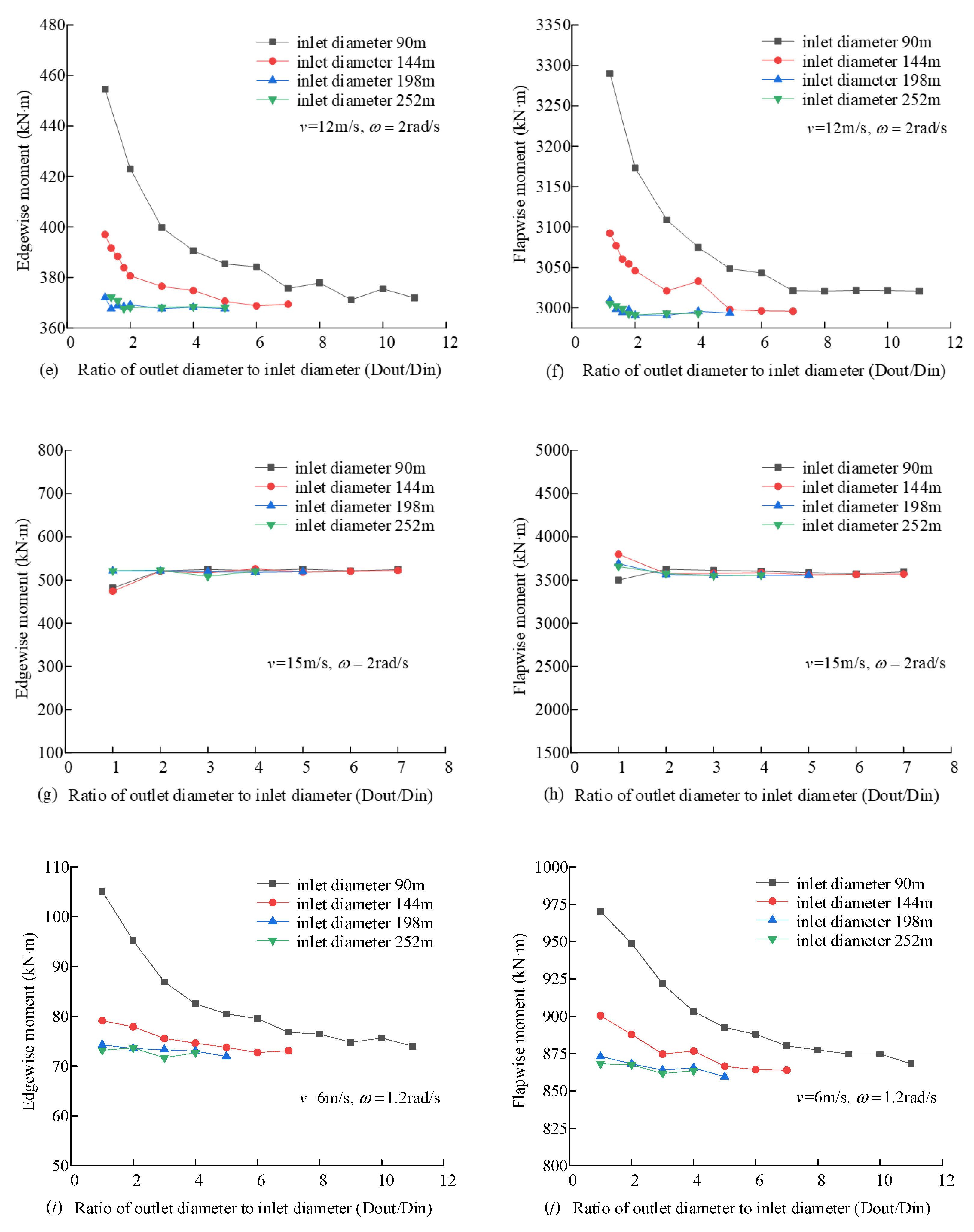
Both edgewise and flapwise moments of the blade are employed as the indicators of the blade load. The calculation results obtained at different outlet-diameter-to-inlet-diameter ratios, when the inlet diameter is respectively 90, 144, 198, and 252 m, are shown in Figure 2. In the calculations, different wind speeds and rotor speeds are also considered in order to understand the influences of the flow field under different environmental and turbine control conditions. Herein, it is necessary to note that wind shear is temporarily not considered in this section in order to concentrate the research on investigating the effect of the flow field on the calculation results.

From Figure 2, it is found that

• the computational accuracy of the edgewise and flapwise moments of the blade is significantly affected by the inlet and outlet diameters of the flow field. Moreover, the lower the wind speed, the more their influences on the results will tend to be.
• the smaller the inlet diameter, the larger the outlet diameter to inlet diameter ratio should be adopted in the calculation. Moreover, a small inlet diameter can decrease the accuracy of the calculation results, especially when the outlet diameter of the flow filed is not large enough.
• both edgewise and flapwise moments of the blade will be reduced when the turbine rotor is slow down. However, the change in rotor speed will not change the tendencies of the curves that reflect the influence of the flow field.
• the amount of CFD calculations is dependent on the number of meshes, while the number of meshes relies on the volume of the flow field. Through comparing the volumes of the flow field as well as the number of meshes obtained at different outlet diameter to inlet diameter ratios, it is found that a sharp cone-shaped flow field should be avoided in CFD calculations especially when the inlet diameter of the flow field is not large enough.

Another notable phenomenon is the negative values of the edgewise moment in Figure 2a. The reason for this is that the wind speed v and rotor speed ω are not matched very well, i.e., when wind speed is 6 m/s, rotor speed should be slower, rather than 2 rad/s, according to the running mechanism of wind turbines [28]. This explanation has been confirmed by the results in Figure 2i,j, where wind speed is 6 m/s and rotor speed is 1.2 rad/s, and the results of both edgewise and flapwise moments are positive values.

3. Impact of Yaw Operation on Wind Turbine Blades

3.1. Blade Loads during Yaw Operation

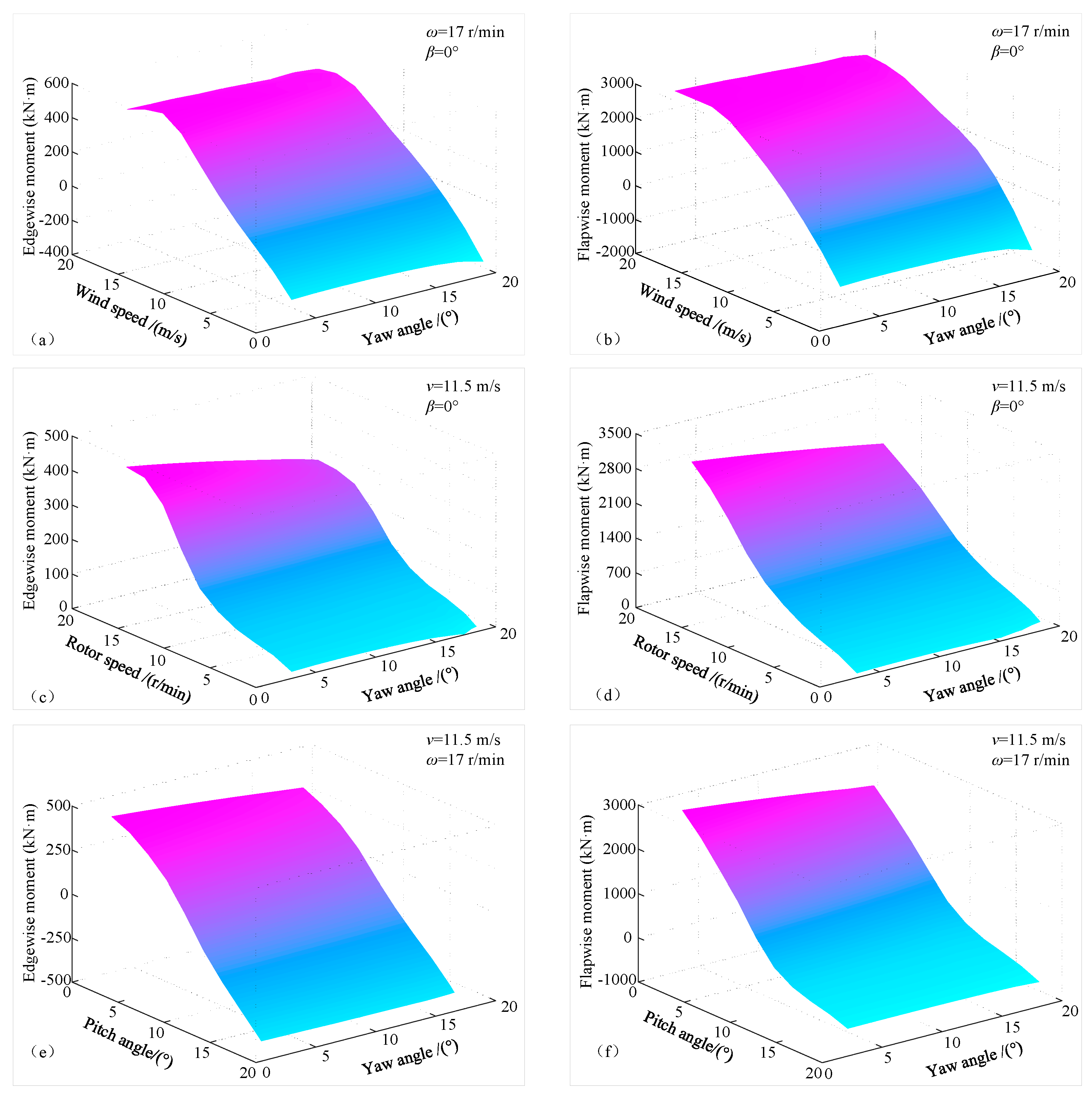
When the wind blows a wind turbine, both edgewise and flapwise bending moments will be created at the root section of the blade. The former will drive the turbine rotor to rotate, while the latter will cause deflection to the blade. Both are not only dependent on wind speed and wind direction but are also influenced by the control parameters of the turbine, such as rotor speed, pitch angle, and yaw angle. To understand the blade loads during the process of yaw operation, both the edgewise and flapwise moments under various combined conditions of wind speed, rotor speed, yaw angle, and pitch angle are calculated. The calculation results are shown in Figure 3. In the subplots, $\mathsf{\omega }$ indicates the rotor speed, $v$ is wind speed, $\beta$ represents pitch angle, and yaw angle γ increases gradually from 0° to 18°.

Figure 3a,b show the influences of yaw operation on blade loads when rotor speed $\omega =$17 r/min, pitch angle $\beta =0^{\mathrm{o}}$, and wind speed $v$ increases gradually from 3 m/s to 19 m/s. From Figure 3a,b it is found that when wind speed $v=$3 m/s, the edgewise moment is negative due to the mismatch of rotor speed and wind speed, and the flapwise moment decreases with the increase of the yaw angle. When wind speed $v=$5 m/s, it is interestingly found that with the increase of the yaw angle, both edgewise and flapwise moments increase first and then decrease. A similar phenomenon is also observed from the edgewise moment obtained when wind speed $v=$7 m/s. By contrast, the flapwise moment obtained at this wind speed decreases monotonously with the increase of the yaw angle. When wind speed varies in the range of [9 m/s, 13 m/s], both edgewise and flapwise moments show a decreasing trend with the increasing yaw angle. When the wind speed $v>$15 m/s, an obvious nonlinearly decreasing trend is observed from the moments in both directions.

Figure 3c,d show the effect of yaw operation on blade loads when wind speed $v=$11.5 m/s, pitch angle $\beta =0^{\mathrm{o}}$, and rotor speed increases gradually from 3 r/min to 19 r/min. From Figure 3c,d, it is found that (1) both edgewise and flapwise moments generally decrease with the increase of yaw angle, and (2) increasing rotor speed will lead to the increase of the bending moments in both directions despite the value of yaw angle. Moreover, the faster the rotor speed, the more the bending moments will increase. The increase rate can be indicated by the gradients of the curves. Let $x$be the yaw angle, and let $y$ be the bending moment in either edgewise or flapwise direction. Then a linear equation $\widehat{y}=ax+b$ can be used to describe the relationship between the yaw angle and the blade loads. After estimating the gradient of the equation using the least-squares method, it is found that when the rotor speed is 3 r/min, the gradient $a=$ 0.58. The value of $a$ increases to 0.95 when rotor speed $v=$11 r/min, 2.5 when $v=$13 r/min, and 6.8 when $v=$19 r/min.

Figure 3e,f show the effect of yaw operation on blade loads when wind speed $v=$11.5 m/s, rotor speed $\omega =$17 r/min, and pitch angle $\beta$ increases gradually from 0° to 16°. From Figure 3e,f, it is found that when pitch angle $\beta <$8°, both edgewise and flapwise moments decrease gradually with the increase of yaw angle. However, the edgewise and flapwise moments show negative values when $\beta >$8° due to the mismatch of wind speed, rotor speed, and pitch angle. In addition, it is found that with the increase of pitch angle, the influence of the yaw angle on the bending moments in both directions decreases. For example, when the pitch angle increases from 0° to 8°, the value of gradient $a$ decreases gradually from 7.0 to 5.0.

3.2. Prediction of the Blade Loads during Yaw Operation

As mentioned earlier, it is very important to the control of hydraulic yaw brake if the blade loads during yaw operation can be predicted. To reach this purpose, mathematical models that reflect the relationship between the blade loads and wind speed, rotor speed, yaw angle, and pitch angle are developed by following the steps below:

Step 1:

Study the effects of individual factors on the blade loads. The factors include yaw angle, wind speed, rotor speed, and pitch angle;

Step 2:

Conduct the orthogonal experiment, i.e., the study of some representative points that are selected from the overall experiment according to the orthogonality;

Step 3:

Develop load models, i.e., the mathematical models of blade loads are developed, of which the variables are wind speed, rotor speed, yaw angle, and pitch angle.

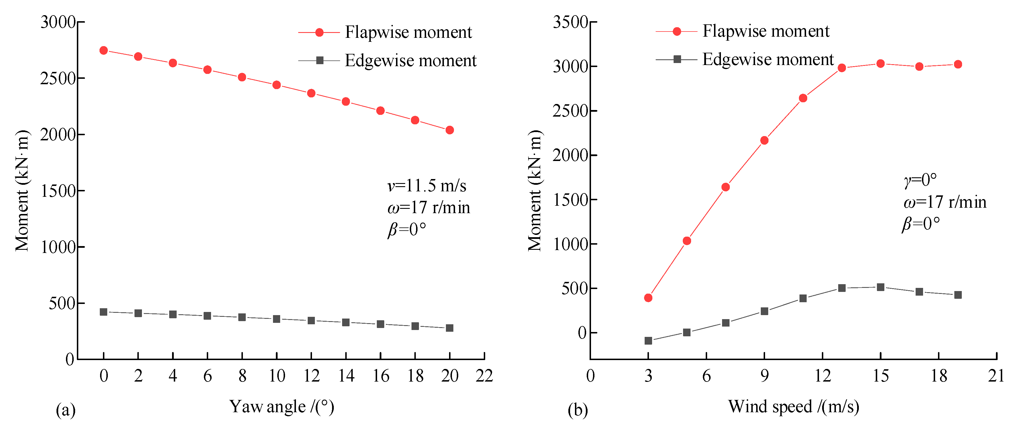
The orthogonal experimental design is a method to study multi-factors and multi-levels. In this method, some representative points are selected from the comprehensive experiments according to the orthogonality. These representative points are “uniform dispersion, uniform comparison”. Renowned Japanese statistician Genichi Taguchi tabulated the horizontal combinations chosen in the orthogonal experiment, called the orthogonal tables. For example, for a three-factor three-level experiment, according to the comprehensive experimental requirements, 3³ = 27 combinations of the experiments are required, which has not yet taken into account the repetition number of each combination. If the experiment is arranged according to the L9 (3³) orthogonal table, it only needs to be conducted nine times. To design the orthogonal experiment by referring to the orthogonal tables, the influences of individual factors are investigated first. Use the results obtained when yaw angle γ = 0°, wind speed v = 11.5 m/s, rotor speed ω = 17 r/min, and pitch angle β = 0° as the references, the influences of individual factors on blade loads are shown in Figure 4.

From Figure 4, it is found that in the considered scenarios, blade loads will decrease with the increase of yaw angle and pitch angle, while they will increase with the increase of wind speed and rotor speed. According to the characteristic of the curve in Figure 4, the four factors of yaw angle, wind speed, rotor speed, and pitch angle are designed as six levels. Considering the influence of the yaw angle and pitch angle on the gradients of the blade load curves is relatively smooth, the yaw angle and pitch angle are designed as six levels based on a uniform distribution, while wind speed and rotor speed are designed as six levels obeying a non-uniform distribution because inflection points can be clearly observed from Figure 4b,c. The resultant factor levels for the orthogonal experiments are listed in

Table 2. Factor levels for the orthogonal experiments.

Level	$\mathit{\gamma }/°$	$\mathit{\nu }/\left(\mathbf{m}/\mathbf{s}\right)$	$\mathsf{\omega }/\left(\mathbf{r}/\mathbf{m}\mathbf{i}\mathbf{n}\right)$	$\mathit{\beta }/°$
1	0	3	3	0
2	4	7	7	3
3	8	11	11	6
4	12	13	15	9
5	16	15	17	12
6	20	19	19	15

.

The level of every factor in Table 2 is divided into two stages in this paper. The first stage includes levels 1, 2, and 3, while the second stage includes levels 4, 5, and 6. A total of 16 sets of L₉ (34) standard orthogonal experiments are designed. For example, when the levels of all four factors are in the first stage, it is the first standard orthogonal experiment table. When the level of pitch angle is in the first stage, and the other three factors are in the second stage, it is the second standard orthogonal experiment table. The design of the other orthogonal experiment tables is developed in the same way. For example,

Table 3. The first set of orthogonal experiments.

Experiment Number	Level of Yaw Angle	Level of Wind Speed	Level of Rotor Speed	Level of Pitch Angle	${\mathit{T}}_1/\left(\mathbf{k}\mathbf{N}\cdot \mathbf{m}\right)$	${\mathit{T}}_1/\left(\mathbf{k}\mathbf{N}\cdot \mathbf{m}\right)$
1	1	1	1	1	14.13	92.404
2	1	2	2	2	116.052	515.703
3	1	3	3	3	295.077	1116.128
4	2	1	2	3	−26.301	−11.035
5	2	2	3	1	145.982	1036.561
6	2	3	1	2	58.571	273.8
7	3	1	3	2	−54.02	26.203
8	3	2	1	3	33.573	139.406
9	3	3	2	1	78.193	598.994

gives the first orthogonal experiment table (T₁ indicates edgewise moment and T₂ indicates flapwise moment).

Subsequently, use variables x₁, x₂, x₃, x₄ to represent yaw angle, wind speed, rotor speed, and pitch angle, and use T₁ to indicate edgewise moment and T₂ flapwise moment, respectively. Then the mathematical models of T₁ and T₂ are established using multiple regression analysis. As opposed to the linear regression analysis, nonlinear regression analysis is more informative. Therefore, a quadratic regression analysis technique is employed here to construct the models. According to the principle of statistical analysis, a complete quadratic regression equation including constant term, linear terms, cross-product terms, and square terms can be expressed as

$$\{\begin{array}{l}{T}_1=c_0+{\displaystyle {\displaystyle \sum }_{i=1}^4}{c}_i{x}_i+{\displaystyle {\displaystyle \sum }_{i=1}^3{\displaystyle \sum }_{j=i+1}^4}{c}_{ij}{x}_i{x}_j+{\displaystyle {\displaystyle \sum }_{i=1}^4}{c}_{ii}{x}_i^2\\ T_2=d_0+{\displaystyle {\displaystyle \sum }_{i=1}^4}{d}_i{x}_i+{\displaystyle {\displaystyle \sum }_{i=1}^3{\displaystyle \sum }_{j=i+1}^4}{d}_{ij}{x}_i{x}_j+{\displaystyle {\displaystyle \sum }_{i=1}^4}{d}_{ii}{x}_i^2\end{array}$$

(1)

where $c_{ij},d_{ij}$are the coefficients to be determined. Then, together with the standard error, the ratio of regression coefficient t can be readily obtained using the least-squares method. The probability of sample observation (or extreme result when the original hypothesis is true) P is calculated by substituting the sample data into the test statistic formula when H0 (also called invalid hypothesis) is assumed to be true. The smaller the value of P, the more likely that the test statistic calculated from the sample point will fall into the rejection domain. Generally, if the value of P is less than 0.05, it is considered that it falls into the rejection domain, and the small probability event occurs. Then, the original assumption can be rejected. The quadratic regression parameter estimates for T₁ and T₂ are listed in

Table 4. Parameter estimates of quadratic regression for T_1.

Variable	Estimated Value	Standard Error	t Value	P Value
Constant term	−109.989	79.7698	−1.3788	0.1703
$x_1$	3.1879	5.8569	0.5443	0.5871
$x_2$	−18.7357	8.2338	−2.2754	0.0245
$x_3$	31.5959	8.6289	3.6616	0.0003
$x_4$	35.5136	7.7962	4.5552	1.2 × 10−5
$x_1{x}_2$	−0.4873	0.2298	−2.1204	0.0358
$x_1{x}_3$	−0.1132	0.213	−0.5317	0.5958
$x_1{x}_4$	0.2654	0.234	1.1341	0.2588
$x_2{x}_3$	3.5584	0.2785	12.7757	1.16 × 10−24
$x_2{x}_4$	1.4949	0.306	4.8848	3.01 × 10−6
$x_3{x}_4$	−4.3281	0.2836	−15.2599	1.11 × 10−30
$x_1^2$	−0.065	0.204	−0.3205	0.749
$x_2^2$	0.4057	0.3072	1.3207	0.1889
$x_3^2$	−2.1032	0.3329	−6.3173	3.97 × 10−9
$x_4^2$	−1.7072	0.3628	−4.7052	6.44 × 10−6

and

Table 5. Parameter estimates of quadratic regression for T_2.

Variable	Estimated Value	Standard Error	t Value	P Value
Constant term	−539.501	232.1584	−2.3238	0.0216
$x_1$	5.6244	17.0458	0.3299	0.7419
$x_2$	6.407	23.9632	0.2673	0.7896
$x_3$	95.5963	25.1133	3.8065	0.0002
$x_4$	65.6491	22.6898	2.8933	0.0044
$x_1{x}_2$	−1.2143	0.6688	−1.8154	0.0717
$x_1{x}_3$	−0.7268	0.6199	−1.1724	0.2431
$x_1{x}_4$	1.2093	0.6811	1.7755	0.0781
$x_2{x}_3$	9.5762	0.8106	11.8133	2.79 × 10−22
$x_2{x}_4$	−2.1539	0.8906	−2.4184	0.0169
$x_3{x}_4$	−13.7124	0.8254	−16.6117	7.65 × 10−34
$x_1^2$	−0.1948	0.5937	−0.3281	0.7433
$x_2^2$	0.8518	0.8942	0.9525	0.3425
$x_3^2$	−2.8406	0.9689	−2.9316	0.0039
$x_4^2$	0.8189	1.056	0.7755	0.4394

, respectively.

Substituting the values of these parameters into (1) gives

$$\begin{gathered} \begin{array}{ll}{T}_1& =-109.989+3.1879x_1-18.7357x_2+31.5959x_3+35.5136x_4-0.4873x_1{x}_2-0.1132x_1{x}_3\\ & +0.2654x_1{x}_4+3.5584x_2{x}_3+1.4949x_2{x}_{4}4.3281x_3{x}_4-0.065x_1^2+0.4057x_2^2-2.1032x_3^2\end{array} \\ -1.7072x_4^2 \\ \begin{array}{ll}{T}_2& =-539.501+5.6244x_1+6.407x_2+95.5963x_3+65.6491x_4-1.2143x_1{x}_2-0.7268x_1{x}_3\\ & +1.2093x_1{x}_4+9.5762x_2{x}_3-2.1539x_2{x}_4-13.7124x_3{x}_4-0.1948x_1^2+0.8518x_2^2\end{array} \\ -2.8406x_3^2+0.8189x_4^2 \end{gathered}$$

(2)

Because there may be multicollinearity between the independent variables in the quadratic regression equation, the method called stepwise regression analysis is further used to modify the quadratic regression equation. The basic idea of stepwise regression analysis is that independent variables are introduced into the model in turn, and then F-test (F-test is used to test the significance of population regression) and t-test are carried out after each new variable is introduced. If the new variable causes the original variable to become less significant, the new variable is deleted to ensure that only significant variables are included in the regression equation. This process is repeated until no significant variable enters the regression equation. After modifying the quadratic regression equation, the parameter estimates of modified quadratic regression for T₁ and T₂ are shown in

Table 6. Parameter estimates of modified quadratic regression for T_1.

Variable	Estimated Value	Standard Error	t Value	P Value
Constant term	−126.153	65.9001	−1.9143	0.0577
$x_2$	−11.5843	4.4283	−2.6159	0.0099
$x_3$	30.3772	8.3611	3.6331	0.0004
$x_4$	38.3866	7.4002	5.1871	7.71 × 10−7
$x_1{x}_2$	−0.3044	0.0957	−3.1783	0.0018
$x_2{x}_3$	3.5391	0.2769	12.7769	6.05 × 10−25
$x_2{x}_4$	1.4918	0.3048	4.8937	2.79 × 10−6
$x_3{x}_4$	−4.3295	0.2819	−15.3572	2.47 × 10−31
$x_3^2$	−2.09	0.3316	−6.3035	3.9 × 10−9
$x_4^2$	−1.7081	0.3615	−4.7248	5.74 × 10−6

and

Table 7. Parameter estimates of modified quadratic regression for T_2.

Variable	Estimated Value	Standard Error	t Value	P Value
Constant term	−503.248	150.9133	−3.3346	0.0011
$x_3$	86.4759	24.1402	3.5822	0.0004
$x_4$	90.53534	14.4742	6.2549	4.89 × 10−9
$x_1{x}_2$	−1.0512	0.2755	−3.8146	0.0002
$x_2{x}_3$	9.6435	0.7354	13.1123	7.61 × 10−26
$x_2{x}_4$	−2.0776	0.8526	−2.4366	0.0161
$x_3{x}_4$	−13.7919	0.8213	−16.791	7.28 × 10−35
$x_2^2$	0.9843	0.4941	1.9916	0.0484
$x_3^2$	−2.7821	0.9659	−2.88	0.0046

, respectively. It is worth noting that the P value of the constant term in the modified equation of quadratic regression for T₁ is 0.0577, which is a little more than 0.05. The item should have been deleted, but since its P value is only slightly larger than 0.05, and once deleted, the item would have a greater impact on the P value of other originally significant variables; hence, this item is retained.

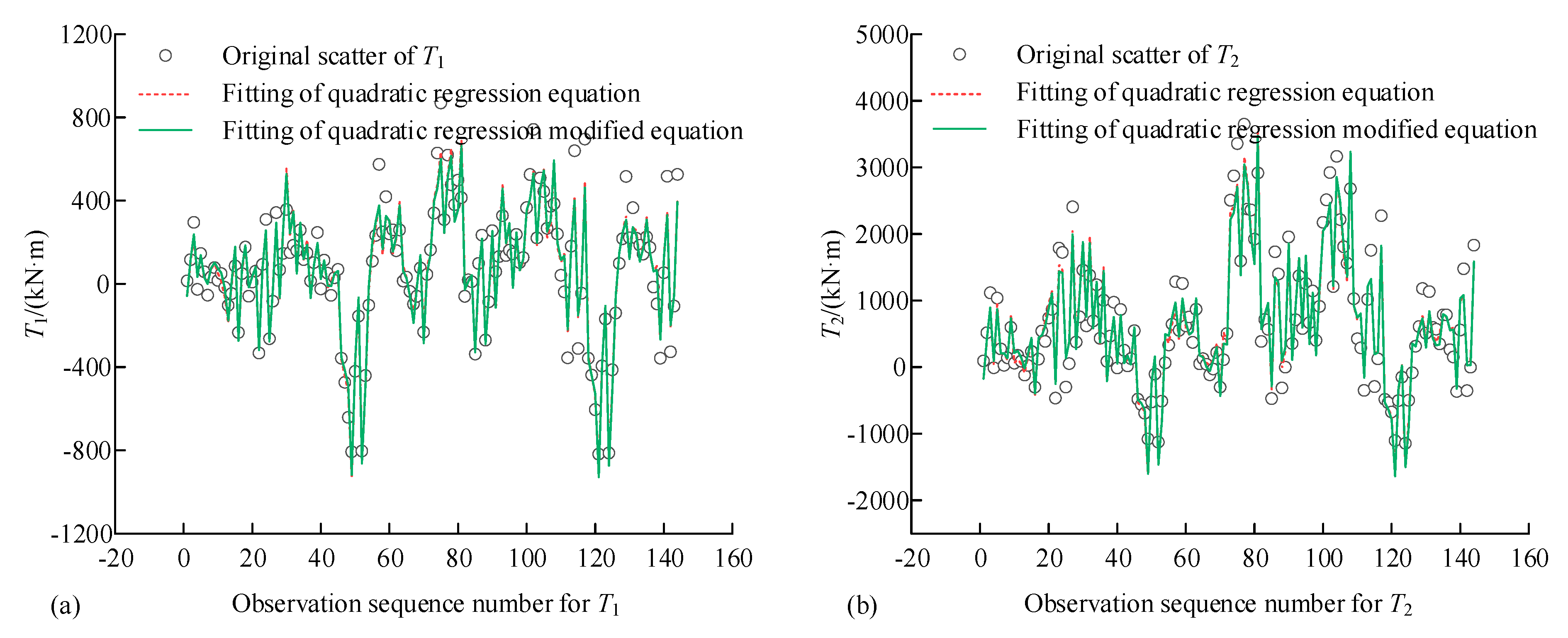
The fitting effect of quadratic regression is shown in Figure 5. The fitting effect difference between the quadratic regression equation and quadratic regression modified equation is not obvious. However, some independent variables appear multicollinearity in the quadratic regression equation, and the modified quadratic regression equation can eliminate the influence of the multicollinearity. Hence, it is reasonable to choose the quadratic regression modified equation as the final expression of the regression equation. As a result, the edgewise moment T₁ and flapwise moment T₂ are expressed as

$$\begin{gathered} \{\begin{array}{l}{T}_1=-126.153-11.5843x_2+30.3772x_3+38.3866x_4-0.3044x_1{x}_2 \\ +3.5391x_2{x}_3+1.4918x_2{x}_4-4.3295x_3{x}_4-2.09x_3^2-1.7081x_4^2\\ T_2=-503.248+86.4759x_3+90.5354x_4-1.0512x_1{x}_2+9.6435x_2{x}_3 \\ -2.0776x_2{x}_4-13.7919x_3{x}_4+0.9843x_2^2-2.7821x_3^2\end{array} \end{gathered}$$

(3)

By using the above analysis method, the loads acting on the blade in both edgewise and flapwise directions can be estimated, i.e.,

$$\begin{gathered} \{\begin{array}{l}{F}_1=-5.2047+0.6044x_1-0.0536x_1{x}_3+0.0525x_2{x}_3+0.0533x_2^2-0.0643x_4^2\\ F_2=-12.9322+2.4262x_3+2.4704x_4-0.0553x_1{x}_2+0.0361x_1{x}_4+0.3563x_2{x}_3 \\ -0.0648x_2{x}_4-0.4508x_3{x}_4+0.0483x_2^2-0.1005x_3^2\end{array} \end{gathered}$$

(4)

where, $F_1$ is the resultant force acting on the blade in the edgewise direction; $F_2$ is the resultant force acting on the blade in the flapwise direction.

4. Impact of Yaw Operation on Energy Capture Performance

4.1. Effects under Different Wind Shear Conditions

Due to the influence of surface roughness, topography, temperature, and other unexpected factors, wind speed is different at different heights above the ground surface, which can cause wind shear. The wind speed profile can be expressed as

$$v\left(z\right)=v_{hub}{\left(\frac{z}{z_{hub}}\right)}^{\alpha }$$

(5)

where $v\left(z\right)$ represents the wind speed at the height of interest z; $z_{hub}$is the hub height of the wind turbine; $\alpha$ is wind shear coefficient; $v_{hub}$is the wind speed measured at hub height.

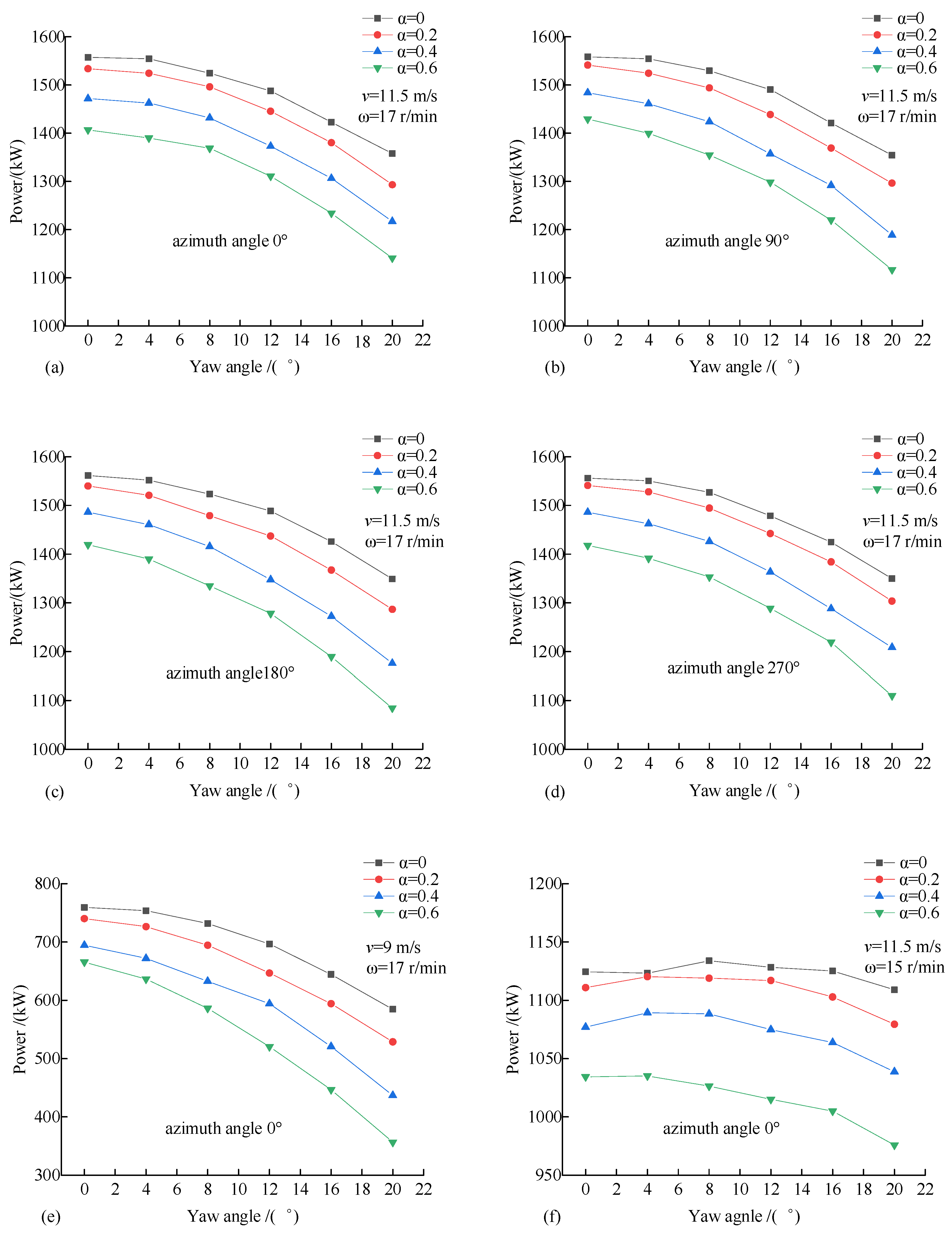
When performing CFD calculations in ANSYS Fluent, a wind speed profile will be applied to describe the wind speeds on the inlet plane of the flow field via a specifically defined user-defined function (UDF) program. Then, when ${\mathrm{z}}_{\mathrm{hub}}=80$ m, the calculation results of the energy captured by the turbine rotor at different wind speeds, rotor speeds, and the azimuth angles of the blade are shown in Figure 6, where Figure 6a–d shows the results obtained when wind speed is 11.5 m/s, the rotor speed is 17 r/min, and the azimuth angle is 0°, 90°, 180°, and 270°, respectively. Figure 6e shows the results obtained when wind speed is 9 m/s, the rotor speed is 17 r/min, and the azimuth angle is 0°. Figure 6f shows the results when wind speed is 11.5 m/s, the rotor speed is 15 r/min, and the azimuth angle is 0°.

From Figure 6a–d, it is found that the energy captured by the wind turbine rotor decreases with the increase of wind shear coefficient, which indicates the negative influence of wind shear on the power production of the wind turbine. To quantitatively describe such negative influence of wind shear, the power fluctuation factor $\mathsf{\Lambda }$ is defined, i.e.,

$$\mathsf{\Lambda }=\frac{P_{\alpha max}-P_{\alpha min}}{P_{\alpha max}}\times 100\%$$

(6)

where $\mathsf{\Lambda }$ indicates the power fluctuation factor when the wind shear coefficient is $\mathsf{\alpha }$; $P_{\alpha max}$ and $P_{\alpha min}$ respectively represent the maximum and minimum energy captured by the turbine rotor during yaw operation.

Apply the power fluctuation factor $\mathsf{\Lambda }$ to assess the calculation results shown in Figure 6. It is found that when the wind shear coefficient increases from 0 to 0.6, the value of $\mathsf{\Lambda }$ increases from 12.82% to 18.91% in Figure 6a and from 13.09% to 21.88% in Figure 6b. The similar increasing tendencies are also found from the power fluctuation factor $\mathsf{\Lambda }$ calculated from other subplots. This fully proves that when the azimuth angle of the blade is constant, the larger the wind shear, the more the energy capture performance of the turbine rotor will be reduced during yaw operation. Moreover, from Figure 6e,f, it is seen that wind shear has always a negative influence on the energy capture performance of the turbine rotor despite wind speed and rotor speed.

Further observation of Figure 6a–d discloses that when the azimuth angle of the blade is different, the obtained power–yaw angle curves are more or less different from each other. This suggests that wind shear can cause fluctuation to the power produced by the wind turbine, which will challenge the power quality of the wind farm if no measures are taken.

4.2. Effects of Blade Deflection

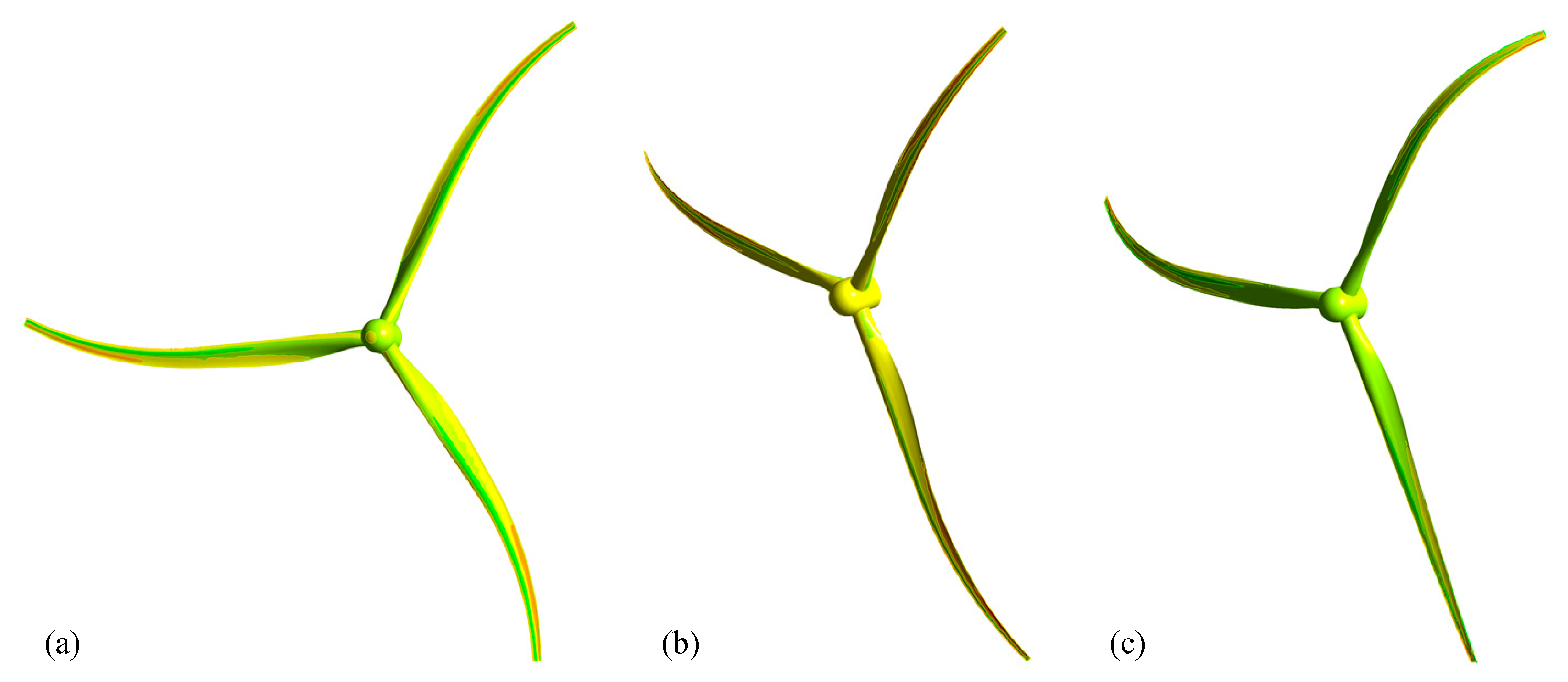
Due to the aerodynamic loads, the wind turbine blades will deflect inevitably, which will affect the energy capture performance of the turbine rotor during yaw operation. To further understand the coupling effects of yaw operation and blade deflection, the energy captured by the wind turbine rotor during yaw operation under different blade deflection conditions are calculated in this section. Considering blade deflection happens mainly from the middle to the tip sections of the blade (see Figure 7), the 3D models of the turbine rotor with deflected blades that are characterized by different deflection angles are established. They are shown in Figure 8. Where Figure 8a is the rotor model when the edgewise deflection of the blade is 30°; Figure 8b is the model when the flapwise deflection of the blade is 30°; Figure 8c shows the model when the blade has 30° deflections in both edgewise and flapwise directions.

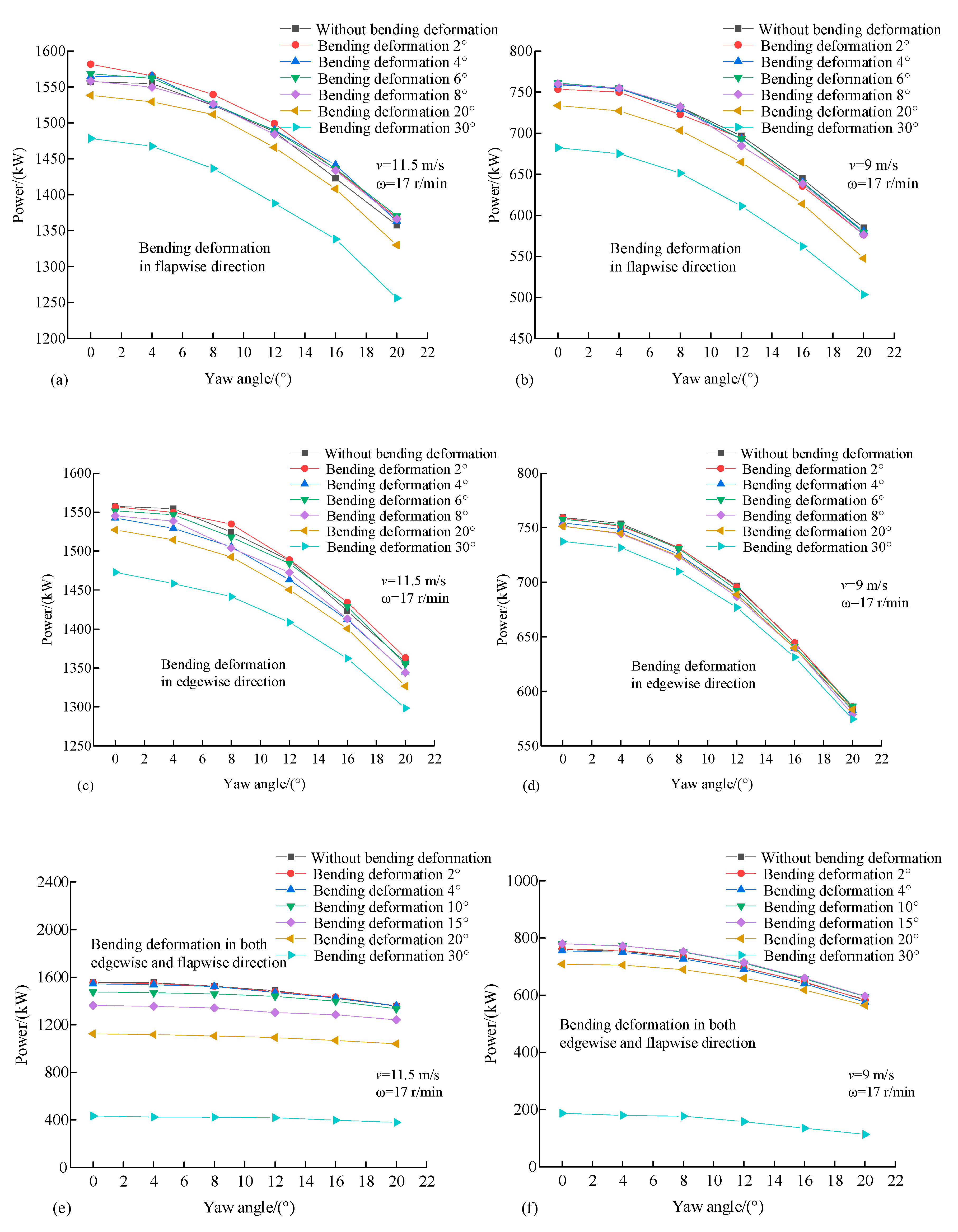
Then the energies captured by the wind turbine rotor during yaw operation under different blade deflection conditions are calculated. The results are shown in Figure 9, where Figure 9a,b shows the results obtained when the rotor speed is 17 r/min, blade deflects in flapwise direction, and wind speed is respectively 11.5 m/s and 9 m/s. Figure 9c,d shows the corresponding results obtained when blade deflects in edgewise direction, while Figure 9e,f shows the corresponding results when the blade deflects in both edgewise and flapwise directions.

From Figure 9, it is found that when wind speed is 9 m/s, the blade’s flapwise deflection has more influence than its edgewise deflection on the energy capture performance of the turbine rotor during yaw operation. For example, when the blade’s flapwise deflection angle is 2°, 4°, 6°, 8°, 20°, and 30°, the corresponding $\mathsf{\Lambda }$ is 23.5%, 23.5%, 23.9%, 24.2%, 25.4%, and 26.0%, respectively, while when the blade’s edgewise deflection angle is 2°, 4°, 6°, 8°, 20°, and 30°, the corresponding $\mathsf{\Lambda }$ is 22.8%, 22.8%, 22.6%, 23.0%, 22.4%, and 22.1%, respectively. From Figure 9, it is interestingly found that the corresponding influence is mitigated when the blade deflects simultaneously in both flapwise and edgewise directions. For example, when wind speed is 9 m/s and 20° deflections occur in both flapwise and edgewise deflections of the blade, the power fluctuation factor $\mathsf{\Lambda }$ is only 20.3%, as opposed to 25.4% when 20° deflection happens only in flapwise direction and 22.4% when 20° deflection happens only in edgewise direction. Moreover, the power fluctuation during yaw operation will be further reduced at higher wind speeds. For example, the corresponding power fluctuation factor $\mathsf{\Lambda }$ is only 7.4% when wind speed is 11.5 m/s and 20° deflections occur in both flapwise and edgewise directions of the blade.

5. Conclusions

To assure the successful implementation of the AWM technology, both blade loads and energy capture performance of wind turbine rotor are investigated in this paper under various combined conditions of wind speed, rotor speed, yaw angle, pitch angle, wind shear, the deflections of the blade, and its azimuth angle. From the research depicted above, the following conclusions can be drawn:

• An appropriate definition of the flow field is critical to the computational efficiency and accuracy of CFD calculations. Through comparing the volumes of the flow field as well as the number of meshes obtained at different outlet-diameter-to-inlet-diameter ratios, it is found that a sharp cone-shaped flow field should be avoided in CFD calculations, especially when the inlet diameter of the flow field is not large enough.
• During yaw operation, the bending moments in both flapwise and edgewise directions of the blade are not only dependent on wind speed, rotor speed, yaw angle, and pitch angle but are also dependent on the matching relationship of them. For example, the bending moments usually decrease with the increase of the yaw angle. However, the bending moments may show a different tendency when wind speed is low. Particularly, when rotor speed and wind speed are mismatched, negative bending moments can be observed.
• With the aid of the orthogonal experiment design, the mathematical models of the blade loads under combined environmental and turbine control conditions are established, which are of great significance to guide the control of the hydraulic yaw brake during yaw operation.
• Wind shear will not only reduce the energy capture performance of the wind turbine rotor but will also cause fluctuation to the power produced by the wind turbine. That will challenge the power quality of the wind farm if no measures are taken.
• A blade’s flapwise and edgewise deflections have different influences on the energy capture performance of the turbine rotor. Usually, the influence of the former is larger than that of the latter. However, it is interestingly found that the corresponding influence is reduced when the blade deflects simultaneously in both flapwise and edgewise directions, especially when wind speed is higher.

Following the above research, the impact of wind turbulence on the aerodynamics and power harvesting performance of the wind turbine rotor during yaw operation will be investigated. The relevant achievements will be reported in separate papers.

References

1. Zheng, W.C.; Li, C.Y.; Pan, J.; Liu, M.Y.; Xia, L.L. An Overview of Global Ocean Wind Energy Resource Evaluations. Renew. Sustain. Energy Rev. 2016, 53, 1240–1251. [Google Scholar] [CrossRef]
2. Zheng, W.C.; Pan, J.; Li, J. Assessing the China Sea Wind Energy and Wave Energy Resources from 1988 to 2009. Ocean Eng. 2013, 65, 39–48. [Google Scholar] [CrossRef]
3. Dai, J.; Yang, X.; Wen, L. Development of Wind Power Industry in China: A Comprehensive Assessment. Renew. Sustain. Energy Rev. 2018, 97, 156–164. [Google Scholar] [CrossRef]
4. McKay, P.; Carriveau, R.; Ting, D.S. Wake Impacts on Downstream Wind Turbine Performance and Yaw Alignment. Wind Energy 2013, 16, 221–234. [Google Scholar] [CrossRef]
5. Archer, L.C.; Vasel-Be-Hagh, A. Wake Steering Via Yaw Control in Multi-Turbine Wind Farms: Recommendations Based on Large-Eddy Simulation. Sustain. Energy Technol. Assess. 2019, 33, 34–43. [Google Scholar] [CrossRef]
6. Lee, H.; Lee, D.J. Wake Impact on Aerodynamic Characteristics of Horizontal Axis Wind Turbine under Yawed Flow Conditions. Renew. Energy 2019, 136, 383–392. [Google Scholar] [CrossRef]
7. José, T.J.; Seifert, J.K.; Würth, I.; Schlipf, D.; Kühn, M. Full-Field Assessment of Wind Turbine near-Wake Deviation in Relation to Yaw Misalignment. Wind Energy Sci. 2016, 1, 41–53. [Google Scholar]
8. Jannik, S.; Bartl, J.M.S.; Mühle, F.V.; Sætran, L.R.; Peinke, J.; Hölling, M. Wind Tunnel Experiments on Wind Turbine Wakes in Yaw: Redefining the Wake Width. Wind Energy Sci. 2018, 3, 257–273. [Google Scholar]
9. Marc, B.; Rott, A.; Beck, H.; Vollmer, L.; Steinfeld, G.; Kühn, M. Field Investigation on the Influence of Yaw Misalignment on the Propagation of Wind Turbine Wakes. Wind Energy 2018, 21, 1011–1028. [Google Scholar]
10. Adaramola, M.S.; Krogstad, P.-A. Experimental Investigation of Wake Effects on Wind Turbine Performance. Renew. Energy 2011, 36, 2078–2086. [Google Scholar] [CrossRef]
11. Shitang, K.; Yu, W.; Wang, T.; Ge, Y. Aerodynamic Performance and Wind-Induced Effect of Large-Scale Wind Turbine System under Yaw and Wind-Rain Combination Action. Renew. Energy 2019, 136, 235–253. [Google Scholar]
12. Simon, B.j.; Mühle, F.V.; Sætran, L.R. Wind Tunnel Study on Power Output and Yaw Moments for Two Yaw-Controlled Model Wind Turbines. Wind Energy Sci. 2018, 3, 489–502. [Google Scholar]
13. Gebraad, P.M.O.; Teeuwisse, F.W.; van Wingerden, J.W.; Fleming, P.A.; Ruben, S.D.; Marden, J.R.; Pao, L.Y. Wind Plant Power Optimization through Yaw Control Using a Parametric Model for Wake Effects—A Cfd Simulation Study. Wind Energy 2016, 19, 95–114. [Google Scholar] [CrossRef]
14. Dongran, S.; Fan, X.; Yang, J.; Liu, A.; Chen, S.; Joo, Y.H. Power Extraction Efficiency Optimization of Horizontal-Axis Wind Turbines through Optimizing Control Parameters of Yaw Control Systems Using an Intelligent Method. Appl. Energy 2018, 224, 267–279. [Google Scholar]
15. Fleming Paul, A.; Ning, A.; Gebraad, P.M.O.; Dykes, K. Wind Plant System Engineering through Optimization of Layout and Yaw Control. Wind Energy 2016, 19, 329–344. [Google Scholar] [CrossRef] [Green Version]
16. Tanvir, A.; Basit, A.; Ahsan, M.; Coupiac, O.; Girard, N.; Kazemtabrizi, B.; Matthews, P.C. Implementation and Analyses of Yaw Based Coordinated Control of Wind Farms. Energies 2019, 12, 1266. [Google Scholar]
17. Min-Soo, J.; Kim, S.W.; Lee, I.; Yoo, S.J.; Park, K.C. The Impact of Yaw Error on Aeroelastic Characteristics of a Horizontal Axis Wind Turbine Blade. Renew. Energy 2013, 60, 256–268. [Google Scholar]
18. Rick, D.; Dana, S.; Annoni, J.; Fleming, P.; Roadman, J.; van Dam, J.; Dykes, K. Assessment of Wind Turbine Component Loads under Yaw-Offset Conditions. Wind Energy Sci. 2018, 3, 173–189. [Google Scholar]
19. Xin, C.; Gu, R.; Pan, P.; Zhu, J. Unsteady Aerodynamics Simulation of a Full-Scale Horizontal Axis Wind Turbine Using Cfd Methodology. Energy Convers. Manag. 2016, 112, 146–156. [Google Scholar]
20. Ok, Y.D.; You, J.Y.; Kwon, O.J. Numerical Investigation of Unsteady Aerodynamics of a Horizontal-Axis Wind Turbine under Yawed Flow Conditions. Wind Energy 2013, 16, 711–727. [Google Scholar]
21. Liping, D.; Zhou, Q.; Zhang, Y.; Yao, S.; Kang, S.; Wang, X. Analysis of Wind Turbine Blades Aeroelastic Performance under Yaw Conditions. J. Wind Eng. Ind. Aerodyn. 2017, 171, 273–287. [Google Scholar]
22. Juchuan, D.; Yang, X.; Hu, W.; Wen, L.; Tan, Y. Effect Investigation of Yaw on Wind Turbine Performance Based on SCADA Data. Energy 2018, 149, 684–696. [Google Scholar]
23. Kragh, K.A.; Hansen, M.H. Load Alleviation of Wind Turbines by Yaw Misalignment. Wind Energy 2014, 17, 971–982. [Google Scholar] [CrossRef]
24. Jeong, M.S.; Cha, M.C.; Kim, S.W.; Lee, I. Numerical Investigation of Optimal Yaw Misalignment and Collective Pitch Angle for Load Imbalance Reduction of Rigid and Flexible Hawt Blades under Sheared Inflow. Energy 2015, 84, 518–532. [Google Scholar] [CrossRef]
25. Ok, Y.D.; Kwon, O.J. Predicting Wind Turbine Blade Loads and Aeroelastic Response Using a Coupled Cfd–Csd Method. Renew. Energy 2014, 70, 184–196. [Google Scholar]
26. Le, P.A.; Lecanu, J. 3d Navier–Stokes Computations of a Stall-Regulated Wind Turbine. Wind Energy Int. J. Prog. Appl. Wind Power Convers. Technol. 2004, 7, 309–324. [Google Scholar]
27. Juchuan, D.; Tan, Y.; Shen, X. Investigation of Energy Output in Mountain Wind Farm Using Multiple-Units SCADA Data. Appl. Energy 2019, 239, 225–238. [Google Scholar]
28. Juchuan, D.; Liu, D.; Wen, L.; Long, X. Research on Power Coefficient of Wind Turbines Based on Scada Data. Renew. Energy 2016, 86, 206–215. [Google Scholar]
Figure 1. The 3D models of the wind turbine. (a) Model of the wind turbine. (b) Model of the blade. (c) Model of the rotor in computational fluid dynamics (CFD).
Applsci 10 01978 g001
Figure 2. Influence of inlet and outlet diameters of the flow field on CFD calculation results.
Applsci 10 01978 g002aApplsci 10 01978 g002b
Figure 3. Aerodynamic loads acting on the blade during yaw operation.
Applsci 10 01978 g003
Figure 4. Influence of individual factors on the aerodynamic load.
Applsci 10 01978 g004aApplsci 10 01978 g004b
Figure 5. Quadratic regression effect fitting.
Applsci 10 01978 g005
Figure 6. Effect of yaw on energy capture under different wind shear conditions.
Applsci 10 01978 g006
Figure 7. Schematic diagram of blade deflections in edgewise and flapwise directions.
Applsci 10 01978 g007
Figure 8. Rotor models with deflected blades, (a) Bending deflection 30° in edgewise direction. (b) Bending deflection 30° in flapwise direction. (c) Bending deflection 30° in both edgewise and flapwise directions.
Applsci 10 01978 g008
Figure 9. Effect of yaw on energy capture under different blade deformations.
Applsci 10 01978 g009