A Machine Learning Method to Estimate Reference Evapotranspiration Using Soil Moisture Sensors

Featured Application

The proposed approach for estimating reference evapotranspiration allows obtaining accurate approximations of this important crop parameter in an inexpensive way by using moisture sensors, which can be translated to an optimization of water resources.

Abstract

One of the most important applications of remote imaging systems in agriculture, with the greatest impact on global sustainability, is the determination of optimal crop irrigation. The methodology proposed by the Food and Agriculture Organization (FAO) is based on estimating crop evapotranspiration (ETc), which is done by computing the reference crop evapotranspiration (ETo) multiplied by a crop coefficient (Kc). Some previous works proposed methods to compute Kc using remote crop images. The present research aims at complementing these systems, estimating ETo with the use of soil moisture sensors. A crop of kikuyu grass (Pennisetum clandestinum) was used as the reference crop. Four frequency-domain reflectometry sensors were installed, gathering moisture information during the study period from May 2015 to September 2016. Different machine learning regression algorithms were analyzed for the estimation of ETo using moisture and climatic data. The values were compared with respect to the ETo computed in an agroclimatic station using the Penman–Monteith method. The best method was the randomizable filtered classifier technique, based on the K* algorithm. This model achieved a correlation coefficient, R, of 0.9936, with a root-mean-squared error of 0.183 mm/day and 6.52% mean relative error; the second-best model used artificial neural networks, with an R of 0.9470 and 11% relative error. Thus, this new methodology allows obtaining accurate and cost-efficient prediction models for ETo, as well as for the water balance of the crops.

1. Introduction

In agricultural sciences, the optimal determination of crop water needs over time is based on measuring the soil water balance and the evaporative demand of the plants. The use of soil moisture measurements was adopted as a suitable strategy for soil water balance estimation. Several methods for computing this balance were developed by different authors [1,2,3]. These techniques were applied in agriculture to obtain the water needs in conjunction with other methods based on remote image sensing. The ultimate objective is to provide farmers with information on the appropriate irrigation volumes to apply in every phenological period of the crop, depending on the desired levels of yield and other parameters. Different physical principles are applied to determine soil moisture, such as gamma-ray spectroscopy [4], synthetic aperture radar [5], and others [6]. Furthermore, there is a wide range of techniques for measuring soil moisture based on electricity, which are applied in geophysical prospecting [7,8] and agronomy [9,10], among other areas. In these measuring techniques, capacitive methods such as frequency-domain reflectometry (FDR) are included [11,12,13]. The accuracy of such sensors varies due to the employed techniques and working conditions.

The key of these techniques is to model the relationships among soil water balance, crop yield, and water use efficiency (WUE) in order to develop better semiarid crops and water management practices [14]. In Mediterranean agriculture, particularly in the southeast of Spain, soil water availability is one of the main limitations for the practice of an economically sustainable agriculture. For this reason, using a suitable irrigation management is critical in the quantity and quality of the obtained harvests. This involves the determination of crop water needs and an optimal irrigation scheduling [15,16,17,18,19]. Although yield reduction is generally expected when crops are subject to limited irrigation, a well-designed limited irrigation system can minimize the impact on yield and still lead to grower profitability.

On the other hand, according to the FAO (Food and Agriculture Organization )-56 methodology [20], crop evapotranspiration (ETc) can be obtained as the product of the reference crop evapotranspiration (ETo) and a crop coefficient (Kc). This Kc coefficient takes into account the development season of the cultivated species, the type of irrigation (by sprinkler, trickle, etc.), and the cultivation techniques (plantation density, pruning, etc.) [21]. Allen et al. [20] proposed Kc values for a great number of species, in standard crop conditions; an adjustment of Kc is necessary when the actual conditions are different from this standard scenario [22,23].

The infrastructure required for a direct measurement of ETc involves high-cost equipment such as lysimeters and Bowen-ratio stations [24]. Therefore, this methodology is unacceptable for small farms. However, both ETo and ETc can also be estimated indirectly, through their relationship with the values obtained using other inexpensive sensors. For example, in the Penman–Monteith method [20], ETo is estimated based on solar radiation, air temperature, humidity, wind speed, atmospheric pressure, site elevation above sea level, Julian day, and latitude degree of the study site. Thus, the main parameters of the soil water state (water content, water potential, and water balance, among others) can be estimated in a cost-efficient way. This methodology is widely extended and used by farmers because of its simplicity. However, it has the disadvantage of giving isolated measurements; in some cases, the obtained parameters are not representative of the entire plot.

To overcome this drawback, remote image capture systems offer a promising alternative to traditional water status measurements [25]. They can provide a snapshot of the whole crop over a reduced period. The advent of unmanned aerial vehicles (UAVs) offers an opportunity to develop remote sensing-based methodologies for precision irrigation [26,27]; they are more affordable than the costly systems based on manned aircrafts, and they provide higher spatial and temporal resolutions than those normally offered by satellites. Various sources of remotely sensed imagery, with differences in spectral, spatial, radioactive, and temporal characteristics, are applied to different purposes of vegetation mapping [28].

Soil moisture sensors are also used to measure the content of water in the soil and provide an estimation of ETc. For example, Sharma et al. [29] applied two different types of sensors based on time-domain reflectometry and capacitance, to estimate the actual evapotranspiration of a greenhouse crop of chili peppers. The final purpose was to reduce the amount of water needed, achieving a reduction of 30%. Other works used soil moisture sensors as a direct way to define irrigation decisions, for example, in crops of tomato [30], turfgrass [31], citrus orchards [32], and other kinds of vegetables [33].

All these facts suggest that it is recommended to combine the FAO-56 methodology with other techniques based on remote images and measurements of the soil water state [34]. Efforts should focus on developing new methods that are more robust, reliable, and sustainable [35,36]. In this paper, the feasibility of estimating ETo using remote sensing techniques based on soil moisture sensors is analyzed. The experiment was performed in a plot in the southeast of Spain, which is an arid zone with a great shortage of water. The proposed methodology integrates different types of inexpensive sensors: meteorological data (daily temperature and rainfall), soil moisture sensors, and irrigation volumes. In order to estimate ETo from the sensor data with high accuracy, a comparison of some advanced pattern recognition techniques is presented. The results of these models are analyzed in detail, selecting the most accurate algorithm. Finally, this estimation of ETo is integrated with an existing methodology for the computation of Kc using remote image sensing [37,38,39], thereby obtaining the daily water balance to adopt the most adequate irrigation decision.

2. Materials and Methods

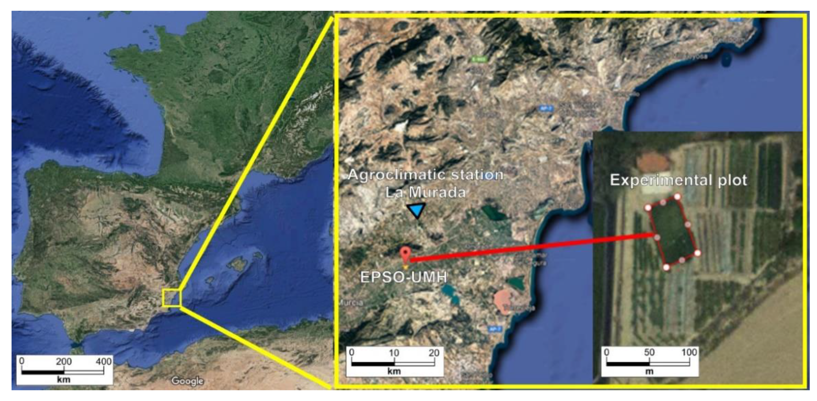
2.1. Data Acquisition

Data collection for this study covered a long period of more than one year, from May 2015 to September 2016. The moisture sensing devices were tested in an experimental plot of 34 m² located in the Higher Polytechnic School of Orihuela (EPSO) of the Miguel Hernández University of Elche (UMH), Spain. Crop rows had a north–south (N–S) orientation. A crop of kikuyu grass (Pennisetum clandestinum) with total coverage of the soil was cultivated on this plot. This species of grass was previously used by many authors in different studies on evapotranspiration (ET) [40], and it was employed in our case as a reference model for directly determining the reference ET (ETo). According to Allen et al. [20], the reference crop is “a hypothetical crop with an assumed height of 0.12 m, a surface resistance of 70 s·m⁻¹, and an albedo of 0.23, closely resembling the evaporation from an extensive surface of green grass of uniform height, actively growing and adequately watered”. All these characteristics are approximately met by the selected species.

The geographical location of the plot is shown in Figure 1. It has a latitude of 38°4′10.17′′ N, longitude 0°59′6.81′′ west (W), and an altitude of 19 m above sea level. The climate in this region is semiarid Mediterranean type, with mild winters and scarce rainfall.

The soil of the experimental plot was loamy in the most superficial layer, with a water field capacity of 0.27 m³/m³ and a permanent wilting point of 0.15 m³/m³. More detailed information of the main soil characteristics is shown in

Table 1. Main characteristics of the soil in the experimental plot at different depths.

Property	0–10 cm	10–20 cm	20–30 cm
Sand (%)	45	61	75
Silt (%)	30	22	16
Clay (%)	25	17	9
Water field capacity (m3/m3)	0.27	0.22	0.18
Permanent wilting point (m3/m3)	0.15	0.12	0.08

. The employed irrigation water had an average quality, with a slightly moderate electrical conductivity and a moderate content of total salts. The plot included a pressure irrigation system with a programmer that provided optimal irrigation to the crop during all the experiment, to meet the requirement of “actively growing and adequately watered”.

The agroclimatic data for the study of the water balance were obtained from the website of the Valencian Institute of Agricultural Research (http://www.ivia.gva.es/en), which uses information taken from the climatic station of La Murada, Orihuela. This station has a latitude of 38°10′51.8′′ N, longitude 0°57′30.8′′ W, and it is installed at 96 m above sea level, as shown in Figure 1; the distance from this station to the experimental crop is approximately 9.5 km. It is a Model 3 station, which is the predominant scheme of the SIAR Network (Agroclimatic Information System for Irrigation) adopted by the Spanish Ministry of Agriculture. This model contains a temperature–humidity sensor, a radiation sensor, a wind speed and direction sensor, a pluviometer, and a datalogger. The main variables used in the current research during the study period are shown in Figure 2, including the daily ETo, mean daily temperature, daily rainfall, and daily irrigation by drip and sprinkler. The last two values were directly obtained from flow meters in the experimental plot. The ETo values from the station were estimated using the Penman–Monteith method [20], and the results were considered as the ground truth.

It can be observed in Figure 2 that daily temperature and ETo are highly correlated, although the ETo cannot be simply deduced from the temperature. The highest values of temperature were obtained in the summer months, from June to September, and the lowest values corresponded to the winter months, from December to March, while the cycle of ETo was slightly displaced, with the highest values from May to July, and the lowest from November to February. Regarding the water supply, it was mostly uniform in the study period, although it decreased around the spring season, with irrigations of less than 7 mm and only one every two days. The total rainfall in this period was 269 mm.

To measure the soil moisture in the study plot, commercial frequency-domain reflectometry (FDR) sensors were used. These FDR sensors consist of several cylindrical rings located at four depths (10, 20, 30, and 40 cm) in an isolated gauge, with a polyvinyl chloride (PVC) access tube of type EnviroSCAN^® (Sentek Sensor Technologies, Stepney, Australia). Four of these gauges were installed spaced in the plot during the experiment. Soil moisture data were collected every 5 min from 30 May 2015 to 30 September 2016. The sensors were firstly installed in the laboratory, where they were tested and calibrated. Afterward, they were installed in the experimental plot. The data obtained from the sensors were stored in data loggers, and then they were collected weekly.

2.2. Data Preparation and Preprocessing

The information considered in the present research consists of the following variables: the measures obtained from the four soil moisture sensors at four different depths; the daily rain, temperature, and ETo measured in the agroclimatic station of La Murada; the amount of irrigation (by sprinkler and drip) applied every day to the reference crop. Recall that the purpose is to estimate ETo using the soil moisture sensors and agroclimatic data. In this way, the additional information required in the proposed approach can be easily obtained using a thermometer and a pluviometer. The total amount of information collected during the period of study contained more than 100 MB. However, some sensors had failures on certain days, providing no information. Therefore, data preprocessing was a very important preliminary step.

On the one hand, it has to be observed that moisture measurements were taken very frequently (288 times per day), while ETo, rainfall, irrigation, and temperature were collected only daily. This can be seen in the sample depicted in Figure 3. Therefore, for each of the four different depths of the sensors, the daily median, average, and standard deviation were computed and used as input features. This way, all the features had daily frequency. In total, there were full data available for 187 days.

In the sample days shown in Figure 3, irrigation was done at approximately 8:30 a.m. every day. At these moments, moisture sensors reached their highest values before quickly decreasing. The rate of decrease was greater with a higher temperature and ETo, as seen in the days from 28 to 30 June 2015. It can also be observed in Figure 3 that no irrigation was applied in the last two days; thus, the soil moisture values continued decreasing, mainly from 12:00 to 6:00 p.m. on both days. To avoid the effect of peaks in the regression algorithms, before computing the statistics, the logarithm of the measures was firstly taken, and then the resulting values were normalized between 0 and 1.

Moreover, since many days were removed because of the missing data, another dataset was generated to test the machine learning algorithms. In this case, we took into account that the evapotranspiration, temperature, moisture, etc. of the crops were not the same throughout the day, but they changed cyclically. Thus, this new dataset was obtained computing the same statistics (median, average, and standard deviation) from the moisture sensors in periods of 6 h, instead of 24 h. This way, for each day of the study, four different samples were generated: 0 to 6 h; 6 to 12 h; 12 to 18 h; 18 to 24 h. Some days presented missing data in these periods; thus, the total number of samples for the 187 days was 682 (i.e., 66 samples were discarded). Since the data of temperature, ETo, and irrigation were available as the mean/total of each day, these values were the same for the four tuples created for each day.

Finally, it was observed that moisture sensor number 3 was responsible for the most missing data. In order to increase the number of available samples, a third dataset was generated. The procedure was the same as in the second dataset, with four periods per day, but without using the data from sensor 3. Consequently, in this dataset, the total number of samples increased to 930.

2.3. Regression Algorithms Used

In general, a regression method is a process to estimate the value of a numerical dependent variable (the output) given a set of independent variables (the input). In machine learning, this regression is not necessarily calculated by a mathematical equation, but by an algorithmic process. In our case, more than 20 machine learning algorithms and variants were applied to train the regression models for the estimation of the reference evapotranspiration, ETo, using the other attributes available: soil moisture sensors at depths 1, 2, 3, and 4; temperature; rainfall; irrigation; day of the year. The last parameter allows the algorithms to model the relationships between the season of the year and the other variables.

Since the purpose of the present research is to select the most accurate regression technique, a detailed description of all the algorithms tested would be outside the scope of this paper, and only the most relevant methods are briefly described. Three scientific tools (one commercial tool and two free tools) were used to test the models before selecting the best one.

• MATLAB 9 (MathWorks Inc., Natick, MA, USA) was used to validate the regression algorithms based on artificial neural networks (ANNs), since it has a powerful ANN toolkit. Specifically, the models used were classical multilayer perceptron ANNs [41]. These networks consist of several input neurons (one for each input variable), one output neuron (the estimation of ETo), and several hidden layers with some neurons per layer. Different configurations were tested in the experiments.
• R 3.4 (R Foundation, Vienna, Austria) is a free programming language and software environment that is very common in scientific computation and statistical analysis. This tool was used to test the algorithms based on support vector regression (SVR) and regression trees (RT). SVR is an adaptation of support vector machines (SVM) to regression problems [42], where a number of relevant samples are selected from the training set (the support vectors) to minimize the error. Similarly, RTs are an adaptation of decision trees [43], where the intermediate nodes perform decisions based on the input variables, and the terminal nodes contain the predicted output values.
• Weka 3.8.1 (The University of Waikato, Hamilton, New Zealand) is a very popular, complete, and free machine learning tool. It contains many classification and regression algorithms that were included in this research. Some of the main techniques are as follows: linear regression; k-nearest neighbors; Bayes networks; logistic regression; K* algorithm; locally weighted learning; rule-based methods; different types of decision trees. Moreover, some meta-algorithms are included; these are algorithms that use other algorithms as parameters. For example, it is worth mentioning the randomizable filtered classifier (RFC) [44], a variant of the filtered classifier that applies an arbitrary transformation to the input data, and then executes another base algorithm on this transformed input. In this way, the regression accuracy could be greater in the filtered input than in the original one.

2.4. Model Validation Measures

As already described, many different combinations of regression methods, variants, and configurations were applied in the experiments to the available datasets. Their results were analyzed using the root-mean-squared error (RMSE) of the obtained predictions for the test set. This error is defined as

$$RMSE\left(m\right)=\sqrt{\frac{1}{n}·{\displaystyle \sum }_{i=1}^n{\left(y\left(i\right)-y_m\left(i\right)\right)}^2},$$

(1)

where m is a given regression model, n is the number of test samples, y(i) is the ETo calculated with the Penman–Monteith method for the i-th sample, and y_m(i) is the estimated value for that sample using the proposed model m. This parameter is a common way to compare the accuracy of different methods, where a model is better when its RMSE is lower. As an alternative, the mean absolute error (MAE) can also be used to assess the accuracy of a method, which is given by

$$MAE\left(m\right)=\frac{1}{n}·{\displaystyle \sum }_{i=1}^{n}abs\left(y\left(i\right)-y_m\left(i\right)\right).$$

(2)

However, both RMSE and MAE by themselves are difficult to interpret unless they are compared with a range of values for predicted variables. For this reason, the mean relative error (MRE) is another good accuracy measure, since it considers the errors with respect to the ground-truth values. It is defined as

$$MRE\left(m\right)=\frac{1}{n}·{\displaystyle \sum }_{i=1}^n\frac{abs\left(y\left(i\right)-y_m\left(i\right)\right)}{y\left(i\right)}.$$

(3)

Finally, another frequently used measure is the correlation coefficient, R, that expresses the linearity in a scatter plot of measured and predicted values of ETo. It can be computed as

$$R\left(m\right)=\frac{{{\displaystyle \sum }}_{i=1}^n\left(y\left(i\right)-\overline{y}\right)·\left(y_m\left(i\right)-\overline{y_m}\right)}{\sqrt{{{\displaystyle \sum }}_{i=1}^n\left(y\left(i\right)-\overline{y}\right)}·\sqrt{{{\displaystyle \sum }}_{i=1}^n\left(y_m\left(i\right)-\overline{y_m}\right)}},$$

(4)

where $\overline{y}$ is the average of y(i) for i in (1…n), and $\overline{y_m}$ is the average of y_m(i) for i in (1…n).

2.5. Remote Image System for the Estimation of the Water Balance

The ultimate goal of the present research is to predict the actual values of the crop evapotranspiration, ETc, which is a part of the water balance equation [37].

$$\Delta W=P+I-E{T}_c-D-R,$$

(5)

where $\Delta W$ is the water balance of the crop of interest in a given period, P is the rainfall, I is the irrigation, D is the drainage, and R is the surface runoff. According to the FAO-56 methodology [20], ETc can be calculated as the product of the reference evapotranspiration, ETo, and a crop coefficient, Kc, which is specific to the type of crop and its growth state. Therefore, the proposed method was designed to be integrated with the remote image capture system presented in Reference [39] to create a complete infrastructure for the computation of the water balance. Some sample views of this system are shown in Figure 4 for a crop of lettuce (Lactuca sativa L) which was used as the crop of interest, while kikuyu grass was used as the reference crop for the estimation of ETo.

The integration was done as follows: firstly, the meteorological data (daily temperature and rainfall), the soil moisture values and the irrigation of the reference crop, and the images of the crop of interest were captured with the corresponding remote modules and transmitted to the local coordinator node via XBee wireless connection [39]. A segmentation algorithm was applied to the images in the coordinator node to separate plants and background [38], as shown in Figure 4c, obtaining the percentage of green cover (PGC). Then, a regression model was applied to estimate Kc from the PGC, as defined in Reference [37]. Additionally, using the present method, ETo was calculated for the reference crop using the obtained data. Additionally, the estimation of ETc for the crop of interest was given by Kc × ETo. The resulting value was applied in Equation (5) to compute the daily water balance in the crop of interest and adopt the most adequate irrigation decisions.

3. Results and Discussion

The tests performed to obtain an accurate estimation technique of ETo using the moisture sensors consisted of the application of all the machine learning methods described in Section 2.3. These methods were applied to the three datasets defined: (i) daily data; (ii) data at 6-h intervals; (iii) data at 6-h intervals but without taking sensor 3 into account. In all the experiments, the data separation was 80% samples for training and the remaining 20% samples for validation. Therefore, in set (i), there were 150 training samples and 37 test samples; in set (ii), there were 546 training and 136 test samples; in set (iii), there were 744 training and 186 test samples.

The description of the experimental results is presented in two parts: first the comparison of the different models, and then the detailed analysis of the best model selected.

3.1. Comparison of the Regression Models

All the machine learning algorithms studied have several configurable hyperparameters, which were adjusted by trial and error to select their optimal configurations. The optimal configuration of the regression models was as follows:

• In the case of the RTs, the algorithm used for construction of the decision trees was Classification and Regression Trees (CART) [43]. Figure 5a shows a graphical representation of the tree obtained for dataset (iii). It can be observed that the temperature is a very important variable in the regression, combined with the average information of some sensors.
• For the SVR algorithm, the kernel function was a radial basis function, while the cost parameter was 4, with a value of epsilon 0.03 and gamma 0.1. These values were obtained using the tune function of R, which performs an optimization of the hyperparameters of the algorithm.
• The best architecture found using the ANN for dataset (iii) is shown in Figure 5b. In the three datasets, the network had an input layer, an output layer with one neuron, and a hidden layer. The ANN for dataset (i) had 10 hidden neurons, and the backpropagation algorithm was a scale conjugate gradient; for datasets (ii) and (iii), there were 15 hidden neurons and the backpropagation algorithm was Levenberg–Marquardt. In the training process, the datasets were divided into training (60%), validation (20%), and testing (20%). In this way, consistency was maintained in the comparison with the other regression methods.
• Regarding the regression models tested in Weka, in dataset (i), the best algorithm was M5 Rules, while, for the other two datasets, the best method was the randomizable filtered classifier (RFC). M5 Rules is an algorithm that uses a separate-and-conquer strategy to construct a list of decisions or rules [45]. In the case of the RFC, the filter applied to the input data is a random projection to a sub-space of less dimensionality, and the base method of RFC is the K* algorithm [46]. This K* (or K-star) algorithm is an instance-based regressing method, where the estimation for a given input is calculated from samples more similar to it, according to a certain similarity function (normally using entropy-based distance functions). A global blend value of 15 was used in this algorithm.

Table 2. Root-mean-squared error (RMSE) in mm/day, for the prediction of the daily ETo using the different regression algorithms on the three datasets defined. RT: regression tree; SVR: support vector regression; ANN: artificial neural network.

Algorithm	(i) Daily Data	(ii) Data at 6-h Intervals	(iii) Data at 6-h Intervals without Sensor 3
RT	0.7000	0.6700	0.6600
Best Weka model	0.4973	0.3567	0.1829
SVR	0.5354	0.4994	0.4043
ANN	0.5481	0.3037	0.2972

shows the RMSE values obtained for all these regression models. In the case of Weka, only the error of the best model is shown for concision; the rest of models produced worse results than those presented in Table 2.

Globally, the smallest error was obtained using Weka’s RFC algorithm with dataset (iii), combined with the K* algorithm, achieving a very low RMSE of 0.1829 mm/day. Concerning the datasets, it can be observed that the data with daily information led to very poor results in all the methods. The optimal RMSE was almost 0.5 mm/day, using M5 Rules in Weka, which was equivalent to a relative error, MRE, of 33.96%. Thus, this arrangement of the data was not adequate to produce good estimations of the reference evapotranspiration. There can be several reasons for this fact. Firstly, the number of samples of this dataset could be insufficient for most of the machine learning methods used. A much larger number of samples could be necessary to improve the accuracy of the methods. However, this would be difficult for practical use of this methodology, requiring too many days of experimentation (in our case, after more than one year of data collection, the training dataset (i) contained only 150 samples). Moreover, since the daily data accumulated information of the peaks and valleys of each day, the loss of information did not allow producing good estimations.

Both datasets at 6-h intervals achieved better results for all the regression methods studied. This indicates that splitting up the data had a positive effect in the accuracy. The number of samples was more than 3 times larger in dataset (ii), and five times larger in the case of dataset (iii). The difference between the results of sets (ii) and (iii) was negligible for the regression trees, SVR, and ANN. That is, these methods were more robust to missing data due to sensor failures. However, for the optimal method, RFC + K*, the RMSE was reduced to half by discarding sensor 3. This fact shows that, since this method is an instance-based regression, the existence of erroneous or incomplete data had a bigger effect on its accuracy. For this reason, it worked much better in dataset (iii).

The second-best method was the ANN, which achieved the lowest RMSE for dataset (ii), with a value of 0.3037 mm/day, improving the accuracy of RFC + K* in this set. This was equivalent to an MRE above 11.3% and an R of 0.924, which is also a very accurate result. However, the improvement in the ANN upon removing sensor 3 was insignificant, reducing RMSE by only 0.0065. The results of the remaining methods were always worse than those of RFC + K* and ANN. This proves the complexity of the problem, indicating that the relationship between ETo and the input parameters cannot be captured with a simple model. Furthermore, the other techniques applied in Weka, such as linear regression, k-nearest neighbors, Bayes networks, and logistic regression, produced even worse results. Figure 4a shows that temperature is a very important parameters, but there are other factors not related to the temperature.

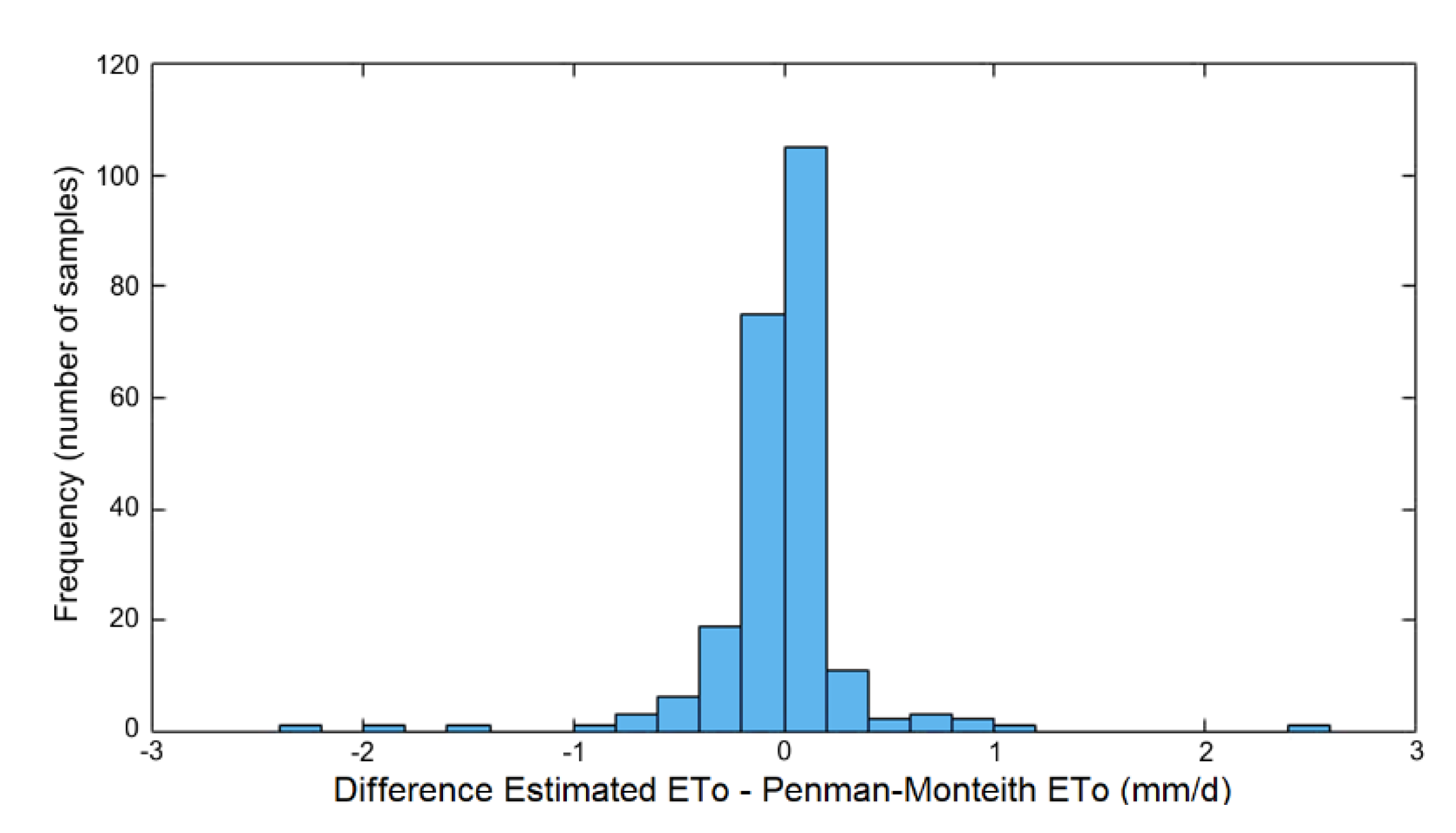
3.2. Accuracy Analysis of the Selected Model

As a result of the previous experiments, the optimal method selected for the estimation of ETo using the moisture sensors and meteorological data was the combination of RFC and the K* algorithm. Recall that this method consists of two steps: firstly, the input tuples are projected into a random subspace of lower dimensionality; then, the K nearest training samples to the input tuple are used to estimate the value of ETo. In this subsection, the results of this method are analyzed in more detail and compared with those of the ANN. The main accuracy parameters are presented in

Table 3. Root-mean-squared error (RMSE) in mm/day, mean absolute error (MAE) in mm/day, mean relative error (MRE), and correlation coefficient (R) for the prediction of the daily ETo using the two best regression algorithms, randomizable filtered classifier with K* algorithm (RFC + K*) and artificial neural network (ANN).

Algorithm	RMSE	MAE	MRE	R
RFC + K*	0.1829	0.0899	6.52%	0.9936
ANN	0.2972	0.1521	11.03%	0.9470

. These measures used the dataset at 6-h intervals removing sensor 3.

Figure 6 shows a comparison of the ETo values estimated using the two best regression models found, compared to the actual values obtained with the Penman–Monteith method in the agroclimatic station of La Murada, for a random subset of evapotranspiration measurements in dataset (iii).

The predictions in Figure 6a are clearly closer to the expected values than those in Figure 6b, in coherence with the error measures. The regression line of the plot in Figure 6a corresponds to the following equation:

$$y=0.9518x+0.1699.$$

(6)

As indicated in Table 3, the correlation of the regression line is 0.9936. Finally, Figure 7 shows a histogram showing the error distribution of the RFC + K* model for the same dataset. Most of the errors were within −1 and +1, with almost no samples having a greater error.

The accuracy measures prove that the proposed method is able to achieve a very precise estimation of ETo, with an average error below 6.5% in relative terms. Thus, a good estimation of ETo can be obtained with a cost-effective system that would only require moisture sensors and agroclimatic data. Since the selected RFC method relies on subspace projections, we performed a principal component analysis (PCA) of the independent variables. It was observed that, from the 43 input variables, the first principal component (PC) accounted for only a 32% of the variance, and the second PC accounted for 13%. This indicates a high complexity in the distribution of the input data. A plot of the dataset (iii) projection in these two components is depicted in Figure 8. The first 10 PCs were required to capture 89% of the variance.

The predicted ETo values are very accurate compared to other estimation methods based on meteorological information of remote imagery. For example, in Reference [47], ETo was estimated using ANN and climatic data (solar radiation, maximum and minimum temperature, maximum and minimum relative humidity, and wind speed) obtaining a weighted standard error of 0.3 mm/day. The Penman–Monteith method was considered as the ground truth, finding that the error of a lysimeter-based method was 0.74 mm/day. Although they used a different accuracy metric, the obtained value was far from the 0.0899 mm/day MAE error achieved with our proposal. Another technique using minimal climatic data (maximum and minimum air temperatures, extraterrestrial radiation, and daylight hours) and ANN was presented in Reference [48], reporting a mean squared error in the daily estimation of 0.356 (mm/day)², which corresponds to an RMSE of 0.597 mm/day. Moreover, Glenn et al. [49] explored several methods of computing ETo using satellite imagery, ground measurements, and meteorological data, observing values of relative root-mean-squared error in the range 10%–30%; again, this is worse than our obtained MRE of 6.5%.

Nevertheless, we consider that more experiments are necessary to verify the excellent results achieved by the proposed method. For example, since the data acquisition was only done in a single configuration, it would be advisable to perform more experiments in different environmental settings, with different climates, crops, ground types, etc. These factors could translate into significant evapotranspiration changes, and this could affect the effectiveness of the generated models. However, even in this case, the same methodology proposed in this article could be followed to obtain and prepare the data, as well as to generate and compare the models.

Finally, it is interesting to observe that the presented model does not consider any prior expert knowledge about the evapotranspiration computation, and it only uses generic machine learning algorithms. Therefore, the application of the proposed methodology to a different environment would be straightforward. It is likely that the results could be further improved in the future upon introducing changes in the model to take into account this expert knowledge.

4. Conclusions

One of the main applications of remote image sensing systems in agriculture is the computation of the optimal irrigation requirements of the crops. For this purpose, estimating the crop evapotranspiration (ETc) is an essential and preliminary step, since it models the water consumption of the crops. In this paper, we presented a new methodology to create precise models that are able to estimate the reference evapotranspiration (ETo) of crops using moisture sensors located in the ground. This estimation of ETo is then integrated with other existing techniques to calculate ETc using remote images and ETo, such as that in Reference [38]. Through the analysis of the aerial images of the crops, the percentage of ground cover is firstly computed, then the crop coefficient is deduced from it, and finally ETc is calculated using ETo and the crop coefficient.

The obtained results indicate that it is possible to obtain a very accurate approximation of ETo using only daily temperature, rainfall, watering and moisture data, and generic machine learning methods. This can be compared with the standard Penman–Monteith method for ETo estimation [20], which requires more climatic data, such as solar radiation, air temperature, humidity, wind speed, and atmospheric pressure, in addition to elevation above sea level, Julian day, and latitude degree of the study site. The high correlation coefficient found between both ETo estimations, over 0.993, and the small mean relative error of 6.5% indicate that this method could be used as an effective substitution of other more expensive solutions, such as lysimeters and Bowen stations, offering a cost-efficient alternative.

As discussed in the paper, this proposal opens new opportunities to experiment with these excellent results under different conditions, for example, in diverse environmental settings, with different climates, varieties of crops, ground types, etc. The proposed methodology consists of obtaining the datasets aggregated at 24- or 6-h intervals, applying different machine learning regression algorithms, and selecting the optimal model and time interval. This procedure would be the same for different conditions, although the best model and the optimal time interval could be dissimilar under those conditions. Another interesting future line is to perform a direct estimation of the ETc of the crop of interest using the moisture sensors, agroclimatic data, and remote image sensing. This would eliminate the need to use a reference crop as a previous step in the process.

References

1. Zhao, J.; Huang, S.; Huang, Q.; Leng, G.; Wang, H.; Li, P. Watershed water-energy balance dynamics and their association with diverse influencing factors at multiple time scales. Sci. Total Environ. 2020, 711, 135189. [Google Scholar] [CrossRef]
2. Ramos, T.B.; Simionesei, L.; Jauch, E.; Almeida, C.; Neves, R. Modelling soil water and maize growth dynamics influenced by shallow groundwater conditions in the Sorraia Valley region, Portugal. Agric. Water Manag. 2017, 185, 27–42. [Google Scholar] [CrossRef]
3. Albaugh, J.M.; Domec, J.C.; Maier, C.A.; Sucre, E.B.; Leggett, Z.H.; King, J.S. Gas exchange and stand-level estimates of water use and gross primary productivity in an experimental pine and switchgrass intercrop forestry system on the Lower Coastal Plain of North Carolina, U.S.A. Agric. For. Meteorol. 2014, 192, 27–40. [Google Scholar] [CrossRef]
4. Filippucci, P.; Tarpanelli, A.; Massari, C.; Serafini, A.; Strati, V.; Alberi, M.; Raptis, K.G.C.; Mantovani, F.; Brocca, L. Soil moisture as a potential variable for tracking and quantifying irrigation: A case study with proximal gamma-ray spectroscopy data. Adv. Water Resour. 2020, 136, 103502. [Google Scholar] [CrossRef]
5. Hosseini, M.; McNairn, H. Using multi-polarization C- and L-band synthetic aperture radar to estimate biomass and soil moisture of wheat fields. Int. J. Appl. Earth Obs. Geoinf. 2017, 58, 50–64. [Google Scholar] [CrossRef]
6. Vienken, T.; Reboulet, E.; Leven, C.; Kreck, M.; Zschornack, L.; Dietrich, P. Field comparison of selected methods for vertical soil water content profiling. J. Hydrol. 2013, 501, 205–212. [Google Scholar] [CrossRef]
7. Sena-Lozoya, E.B.; González-Escobar, M.; Gómez-Arias, E.; González-Fernández, A.; Gómez-Ávila, M. Seismic exploration survey northeast of the Tres Virgenes Geothermal Field, Baja California Sur, Mexico: A new Geothermal prospect. Geothermics 2020, 84, 101743. [Google Scholar] [CrossRef]
8. Linck, R.; Fassbinder, J.W.E. Determination of the influence of soil parameters and sample density on ground-penetrating radar: A case study of a Roman picket in Lower Bavaria. Archaeol. Anthropol. Sci. 2014, 6, 93–106. [Google Scholar] [CrossRef]
9. Banerjee, K.; Krishnan, P. Normalized Sunlit Shaded Index (NSSI) for characterizing the moisture stress in wheat crop using classified thermal and visible images. Ecol. Indic. 2020, 110, 105947. [Google Scholar] [CrossRef]
10. Fatás, E.; Vicente, J.; Latorre, B.; Lera, F.; Viñals, V.; López, M.V.; Blanco, N.; Peña, C.; González-Cebollada, C.; Moret-Fernández, D. TDR-LAB 2.0 Improved TDR Software for Soil Water Content and Electrical Conductivity Measurements. Procedia Environ. Sci. 2013, 19, 474–483. [Google Scholar] [CrossRef] [Green Version]
11. Chen, L.; Zhangzhong, L.; Zheng, W.; Yu, J.; Wang, Z.; Wang, L.; Huang, C. Data-driven calibration of soil moisture sensor considering impacts of temperature: A case study on FDR sensors. Sensors 2019, 19, 4381. [Google Scholar] [CrossRef] [PubMed] [Green Version]
12. Oates, M.J.; Ramadan, K.; Molina-Martínez, J.M.; Ruiz-Canales, A. Automatic fault detection in a low cost frequency domain (capacitance based) soil moisture sensor. Agric. Water Manag. 2017, 183, 41–48. [Google Scholar] [CrossRef]
13. Al-Asadi, R.A.; Mouazen, A.M. Combining frequency domain reflectometry and visible and near infrared spectroscopy for assessment of soil bulk density. Soil Tillage Res. 2014, 135, 60–70. [Google Scholar] [CrossRef] [Green Version]
14. Wiedenfeld, R.P. Water stress during different sugarcane growth periods on yield and response to N fertilization. Agric. Water Manag. 2000, 43, 173–182. [Google Scholar] [CrossRef]
15. Ratnakumar, P.; Khan, M.I.R.; Minhas, P.S.; Farooq, M.A.; Sultana, R.; Per, T.S.; Deokate, P.P.; Khan, N.A.; Singh, Y.; Rane, J. Can plant bio-regulators minimize crop productivity losses caused by drought, salinity and heat stress? An integrated review. J. Appl. Bot. Food Qual. 2016, 89, 113–125. [Google Scholar]
16. Osman, H.; Ammar, M.; El-Said, M. Optimal scheduling of water network repair crews considering multiple objectives. J. Civ. Eng. Manag. 2017, 23, 28–36. [Google Scholar] [CrossRef]
17. Al-Karadsheh, E. Precision Irrigation: New strategy irrigation water management. In Proceedings of the Conference on International Agricultural Research for Development, Deutscher Tropentag, Wiltzenhausen, Germany, 9–11 October 2002; pp. 1–7. [Google Scholar]
18. Evans, R.G.; Buchleiter, G.W.; Sadler, E.J.; King, B.A.; Harting, G.B. Controls for precision irrigation with self propelled systems. In Proceedings of the 4th Decennial Symposium, Phoenix, AZ, USA, 14–16 November 2000. [Google Scholar]
19. Sadler, E.J.; Evans, R.G.; Stone, K.C.; Camp, C.R. Opportunities for conservation with precision irrigation. J. Soil Water Conserv. 2005, 60, 371–379. [Google Scholar]
20. Allen, R.G.; Pereira, L.S.; Raes, D.; Smith, M. Crop evapotranspiration—Guidelines for computing crop water requirements—FAO Irrigation and drainage paper 56; FAO—Food and Agriculture Organization of the United Nations: Rome, Italy, 1998; ISBN 92-5-104219-5. [Google Scholar]
21. Doorenboos, J.; Pruitt, W.O. Guidelines for Predicting Crop Water Requirements, Irrigation and Drainage Paper 24; Food and Agriculture Organization of the United Nations: Rome, Italy, 1977; ISBN 92-5-100279-7. [Google Scholar]
22. Aydin, Y. Determination of reference ETo by using different Kp equations based on class a pan evaporation in southeastern anatolia project (GAP) region. Appl. Ecol. Environ. Res. 2019, 17, 15117–15129. [Google Scholar]
23. Kato, T.; Kamichika, M. Determination of a crop coefficient for evapotranspiration in a sparse sorghum field. Int. Comm. Irrig. Drain. 2006, 55, 165–175. [Google Scholar] [CrossRef]
24. Crago, R.; Brutsaert, W. Daytime evaporation and the self-preservation of the evaporative fraction and the Bowen ratio. J. Hydrol. 1996, 178, 241–255. [Google Scholar] [CrossRef]
25. Huang, Y.; Chen, Z.X.; Yu, T.; Huang, X.Z.; Gu, X.F. Agricultural remote sensing big data: Management and applications. J. Integr. Agric. 2018, 17, 1915–1931. [Google Scholar] [CrossRef]
26. Mogili, U.R.; Deepak, B.B.V.L. Review on Application of Drone Systems in Precision Agriculture. Procedia Comput. Sci. 2018, 133, 502–509. [Google Scholar] [CrossRef]
27. Maes, W.H.; Steppe, K. Perspectives for Remote Sensing with Unmanned Aerial Vehicles in Precision Agriculture. Trends Plant Sci. 2019, 24, 152–164. [Google Scholar] [CrossRef] [PubMed]
28. Xie, Y.; Sha, Z.; Yu, M. Remote sensing imagery in vegetation mapping: A review. J. Plant Ecol. 2008, 1, 9–23. [Google Scholar] [CrossRef]
29. Sharma, H.; Shukla, M.K.; Bosland, P.W.; Steiner, R. Soil moisture sensor calibration, actual evapotranspiration, and crop coefficients for drip irrigated greenhouse chile peppers. Agric. Water Manag. 2017, 179, 81–91. [Google Scholar] [CrossRef] [Green Version]
30. Vázquez, N.; Huete, J.; Pardo, A.; Suso, M.L.; Tobar, V. Use of soil moisture sensors for automatic high frequency drip irrigation in processing tomato. In Proceedings of the XXVIII International Horticultural Congress on Science and Horticulture for People (IHC2010): International Symposium on 922, Lisbon, Portugal, 22–27 August 2010; pp. 229–235. [Google Scholar]
31. Shedd, M.; Dukes, M.D.; Miller, G.L. Evaluation of evapotranspiration and soil moisture-based irrigation control on turfgrass. In Proceedings of the World Environmental and Water Resources Congress 2007: Restoring Our Natural Habitat, Tampa, FL, USA, 15–19 May 2007; pp. 1–21. [Google Scholar]
32. O’Connell, N.V.; Snyder, R.L. Monitoring soil moisture with inexpensive dialectric sensors (Echoprobe) in a citrus orchard under low volume irrigation. In Proceedings of the IV International Symposium on Irrigation of Horticultural Crops 664, Davis, CA, USA, 1–6 September 2003; pp. 445–451. [Google Scholar]
33. Thompson, R.B.; Gallardo, M.; Valdez, L.C.; Fernández, M.D. Using plant water status to define threshold values for irrigation management of vegetable crops using soil moisture sensors. Agric. Water Manag. 2007, 88, 147–158. [Google Scholar] [CrossRef]
34. Carlson, T.N.; Petropoulos, G.P. A new method for estimating of evapotranspiration and surface soil moisture from optical and thermal infrared measurements: The simplified triangle. Int. J. Remote Sens. 2019, 40, 7716–7729. [Google Scholar] [CrossRef]
35. Krishna, P.R. Evapotranspiration and agriculture—A review. Agric. Rev. 2019, 40, 1–11. [Google Scholar]
36. Niu, H.; Zhao, T.; Wang, D.; Chen, Y. Estimating Evapotranspiration with UAVs in Agriculture: A Review. In Proceedings of the 2019 ASABE Annual International Meeting; American Society of Agricultural and Biological Engineers, Boston, MA, USA, 7–10 July 2019; p. 1. [Google Scholar]
37. Escarabajal-Henarejos, D.; Molina-Martínez, J.M.; Fernández-Pacheco, D.G.; Cavas-Martínez, F.; García-Mateos, G. Digital photography applied to irrigation management of Little Gem lettuce. Agric. Water Manag. 2015, 151, 148–157. [Google Scholar] [CrossRef]
38. García-Mateos, G.; Hernández-Hernández, J.L.; Escarabajal-Henarejos, D.; Jaén-Terrones, S.; Molina-Martínez, J.M. Study and comparison of color models for automatic image analysis in irrigation management applications. Agric. Water Manag. 2015, 151, 158–166. [Google Scholar] [CrossRef]
39. Mateo-Aroca, A.; García-Mateos, G.; Ruiz-Canales, A.; Molina-García-Pardo, J.M.; Molina-Martínez, J.M. Remote Image Capture System to Improve Aerial Supervision for Precision Irrigation in Agriculture. Water 2019, 11, 255. [Google Scholar] [CrossRef] [Green Version]
40. Barton, L.; Wan, G.G.Y.; Buck, R.P.; Colmer, T.D. Nitrogen increases evapotranspiration and growth of a warm-season turfgrass. Agron. J. 2009, 101, 17–24. [Google Scholar] [CrossRef]
41. Baum, E.B. On the capabilities of multilayer perceptrons. J. Complex. 1988, 4, 193–215. [Google Scholar] [CrossRef] [Green Version]
42. Drucker, H.; Burges, C.J.C.; Kaufman, L.; Smola, A.J.; Vapnik, V. Support vector regression machines. In Proceedings of the Advances in Neural Information Processing Systems, Denver, CO, USA, 5 May 1997; pp. 155–161. [Google Scholar]
43. Breiman, L. Classification and Regression Trees; Routledge: Abingdon, UK, 2017; ISBN 1351460498. [Google Scholar]
44. Pak, I.; Teh, P.L. Machine learning classifiers: Evaluation of the performance in online reviews. Indian J. Sci. Technol. 2016, 9, 1–9. [Google Scholar] [CrossRef]
45. Holmes, G.; Hall, M.; Prank, E. Generating rule sets from model trees. In Proceedings of the Australasian Joint Conference on Artificial Intelligence, Sydney, NSW, Australia, 6–10 December 1999; pp. 1–12. [Google Scholar]
46. Painuli, S.; Elangovan, M.; Sugumaran, V. Tool condition monitoring using K-star algorithm. Expert Syst. Appl. 2014, 41, 2638–2643. [Google Scholar] [CrossRef]
47. Kumar, M.; Raghuwanshi, N.S.; Singh, R.; Wallender, W.W.; Pruitt, W.O. Estimating evapotranspiration using artificial neural network. J. Irrig. Drain. Eng. 2002, 128, 224–233. [Google Scholar] [CrossRef]
48. Zanetti, S.S.; Sousa, E.F.; Oliveira, V.P.; Almeida, F.T.; Bernardo, S. Estimating evapotranspiration using artificial neural network and minimum climatological data. J. Irrig. Drain. Eng. 2007, 133, 83–89. [Google Scholar] [CrossRef]
49. Glenn, E.P.; Nagler, P.L.; Huete, A.R. Vegetation index methods for estimating evapotranspiration by remote sensing. Surv. Geophys. 2010, 31, 531–555. [Google Scholar] [CrossRef]
Figure 1. Location of the experimental plot in the Higher Polytechnic School of Orihuela (EPSO) of the Miguel Hernández University of Elche (UMH), Spain, and the agroclimatic station of La Murada, Orihuela. Aerial images were extracted from Google Maps.
Applsci 10 01912 g001
Figure 2. Main agroclimatic and irrigation variables during the study period. The agroclimatic variables were obtained in the station of La Murada; irrigation was obtained in the crop. (a) Daily values of the temperature and reference evapotranspiration (ETo). (b) Daily values of the water supply by irrigation and rainfall.
Applsci 10 01912 g002
Figure 3. Sample values of the moisture sensors and agroclimatic data for a period of eight days from 26 June 2015 to 4 July 2015. The values of sensor 1 are shown in this plot. Depth 1: 10 cm; depth 2: 20 cm; depth 3: 30 cm; depth 4: 40 cm.
Applsci 10 01912 g003
Figure 4. Sample images of the remote image system where the proposed method was integrated. (a) Global view of the lettuce crop and a remote image capture module. (b) Sample image captured by the remote module. (c) Segmentation of the previous image in plant and soil.
Applsci 10 01912 g004
Figure 5. Two of the regression methods studied. (a) Trained structure of the regression tree for dataset (iii); in each leaf node, the regression value and the number n of samples is shown. (b) Scheme of the artificial neural network designed for dataset (iii).
Applsci 10 01912 g005
Figure 6. Scatter plots of the reference evapotranspiration (ETo) obtained with the Penman–Monteith method, and the generated predictions using the dataset at 6-h intervals removing sensor 3, applying the two best models. (a) randomizable filtered classifier and K* algorithm; (b) artificial neural network.
Applsci 10 01912 g006
Figure 7. Error histogram of the RFC + K* regression model in the estimation of ETo.
Applsci 10 01912 g007
Figure 8. Projection of the samples in dataset (iii) into the subspace of the two first principal components, PC1 and PC2. The size of the points is proportional to the corresponding ETo values.
Applsci 10 01912 g008