Article

A Novel and Effective Image Super-Resolution Reconstruction Technique via Fast Global and Local Residual Learning Model †

1
College of Communication Engineering, Jilin University, Changchun 130012, China
2
Department of Electronic Information, Zhuhai College of Jilin University, Zhuhai 519041, China
*
Author to whom correspondence should be addressed.
This paper is an extended version of paper published in the 2019 IEEE 4th International Conference on Image, Vision and Computing (ICIVC), Xiamen, China, 5–7 July 2019.
Appl. Sci. 2020, 10(5), 1856; https://doi.org/10.3390/app10051856
Submission received: 3 February 2020 / Revised: 25 February 2020 / Accepted: 2 March 2020 / Published: 8 March 2020

Abstract

:

Featured Application

Application areas of image super-resolution: surveillance, medical diagnosis, Earth observation and remote sensing, astronomical observation, biometric information identification.

Abstract

The principle of image super-resolution reconstruction (SR) is to pass one or more low-resolution (LR) images through information processing technology to obtain the final high-resolution (HR) image. Convolutional neural networks (CNN) have achieved better results than traditional methods in the process of an image super-resolution reconstruction. However, if the number of neural network layers is increased blindly, it will cause a significant increase in the amount of calculation, increase the difficulty of training the network, and cause the loss of image details. Therefore, in this paper, we use a novel and effective image super-resolution reconstruction technique via fast global and local residual learning model (FGRLR). The principle is to directly train a low-resolution small image on a neural network without enlarging it. This will effectively reduce the amount of calculation. In addition, the stacked local residual block (LRB) structure is used for non-linear mapping, which can effectively overcome the problem of image degradation. After extracting features, use 1 × 1 convolution to perform dimensional compression, and expand the dimensions after non-linear mapping, which can reduce the calculation amount of the model. In the reconstruction layer, deconvolution is used to enlarge the image to the required size. This also reduces the number of parameters. We use skip connections to use low-resolution information for reconstructing high-resolution images. Experimental results show that the algorithm can effectively shorten the running time without affecting the quality of image restoration.

Graphical Abstract

1. Introduction

In recent years, with the impact of the Internet boom and the rapid development of information technology, people’s requirements for signal and information processing have gradually increased, and image processing is an important part of information processing. Additionally, image super-resolution (SR) technology is particularly important in image processing. The principle is to pass one or more low-resolution (LR) images to the final high-resolution (HR) image through information processing technology. The traditional method is to enlarge the LR small image to the required size by interpolation, and then use the reconstruction algorithm to obtain an HR image. The super-resolution reconstructed image has clear details and contains plenty of information, so it can be widely used [1,2]. For example, in the crime scene video, HR images provide more favorable evidence for the public security organs’ investigation. In satellite imaging applications such as remote sensing and resource detection, HR images can easily distinguish between two or more similar objects. In medicine, HR images can provide doctors with a more accurate basis for diagnosis, and, thereby, greatly improves diagnostic accuracy. Therefore, an image super-resolution algorithm has great research value.
At present, there are many algorithms for super-resolution (SR). In the research of interpolation-based image super-resolution reconstruction algorithms, the input LR image is mainly denoised, deblurred, and up-sampled to improve the image resolution. Among them, the more classic interpolation algorithms include: the nearest neighbor interpolation, the linear interpolation, the bicubic interpolation, and the spline interpolation [3]. The most classic dictionary-based sr algorithm is sparse encoding [4], which seeks a sparse representation of LR input image blocks and then uses the coefficients of this sparse representation to generate HR output. The LapSRN [5] model based on the pyramid algorithm was proposed by Wei ShengLai et al. It is special in that it introduces a hierarchical network. Each level only doubles the original image and adds the residuals to get a result. The learning-based image super-resolution algorithm mainly learns the similarity between high-resolution and low-resolution image blocks, and generates low-resolution image blocks to be processed into corresponding high-resolution image blocks. It is mainly learned through convolutional neural networks. First, ChaoDong et al. applied a convolutional neural network to image super-resolution reconstruction, which is called a super-resolution convolutional neural network (SRCNN) [6]. The network well implements end-to-end image reconstruction. The hidden layer of the convolutional neural network (CNN) completes all feature extraction and aggregation, but SRCNN does not consider any self-similarities. Since then, more people have proposed image super-resolution algorithms based on CNN. For example, another algorithm a Accelerating the Super-Resolution Convolutional Neural Network (FSRCNN) proposed by ChaoDong et al. [7]. Compared with SRCNN, this algorithm does not need to use interpolation to enlarge the original LR images, but process these directly. Its advantage is to shorten the training time by reducing the picture size. In addition, Wenzhe Shi et al. proposed the Real-Time Single Image and Video Super-Resolution Using an Efficient Sub-Pixel Convolutional Neural Network (ESPCN) [8] model. This model is based on small images for training. The experimental results of super-resolution processing of real-time video are very ideal. The Accurate Image Super-Resolution Using Very Deep Convolutional Networks(VDSR) [9] model was proposed by Jiwon Kim et al. Its input is divided into two parts. One part is to take the entire original images as input, and the other part is to train the residuals and get input. We add the two parts together to get HR images, which greatly speeds up the training and converges better. Afterward, Jiwon Kim proposed Deeply-Recursive Convolutional Network for Image Super-Resolution(DRCN) [10]. This network consists of three parts. However, at the layer of non-linear mapping, it uses a recursive network. The data can loop through the layer multiple times. Unrolling this loop is equivalent to multiple convolutional layers in series using the same set of parameters. Ying Tai et al. proposed the Image Super-Resolution via Deep Recursive Residual Network (DRRN) [11] model. In this model, you can see the shadow of DRCN and VDSR. It uses a deeper network structure to improve performance. There are many picture enhancement layers. It can be understood that a blurry image passes through multiple enhancement layers, which becomes clearer one by one, and obtains a HR image. Tong Tong et al. proposed SRDenseNet [12], which introduced a Desent Block structure. The feature values trained by the upper layer of the network will be passed to the next layer of the network. All features will be connected in series. The benefits of this structure are to reduce the problem of gradient disappearance and reduce parameters. This paper mainly uses an image super-resolution reconstruction technique via a fast global and local residual learning mode (FGLRL). The purpose is to increase the resolution of the image by increasing the width of the network and increase the speed of the algorithm.
This article is divided into five chapters. The first chapter mainly describes the introduction, which introduces several existing methods of image SR. The second chapter mainly describes the structure and ideas of multiple papers related to this paper. The details of the algorithm in this paper are described in Section 3. The fourth section shows the experimental results. The last chapter summarizes the full text.

2. Related Work

2.1. SRCNN((Super-Resolution Convolutional Neural Network)

The SRCNN [6] is a pioneering work of applying CNN to image super-resolution reconstruction. It mainly implements end-to-end mapping of LR images to HR images.
The specific algorithm principle is as follows.
(1) Feature extraction:
The main purpose of feature extraction is to extract image blocks from low-resolution images. At this time, the dimensions of feature vectors are still in low-dimensional space. This is the process of the first convolution. The specific formula is as follows.
F 1 ( Y ) = f ( ω 1 Y + B 1 ) ,
In the formula, Y is a low-resolution input image. ω 1 is a convolution kernel, and B 1 is a bias, where the number of convolution kernels is n 1 . The size is c × f 1 × f 1 , and c is the number of channels, which is set to 1. f is the activation function. The activation function used in this case is Rectified Linear Unit (ReLU), that is f ( x ) = max ( 0 , x ) .
(2) Non-linear mapping:
The purpose of non-linear mapping is to map the extracted low-dimensional features to high-dimensional features. This process is a second convolution. The specific formula is as follows.
F 2 ( Y ) = f ( ω 2 F 1 ( Y ) + B 2 ) ,
Based on the formula, the non-linear mapping is performed on the basis of feature extraction, and ω 2 is the convolution kernel of the non-linear mapping. Since the number of convolution kernels represents the feature vector dimension, n 2 > n 1 , and B 2 represents the bias.
(3) Image reconstruction:
The image reconstruction process is equivalent to convolution using the mean convolution kernel. This is the third layer of convolution. The specific formula is as follows.
F ( Y ) = ω 3 F 2 ( Y ) + B 3 ,
F ( Y ) is the final reconstructed image, ω 3 is the convolution kernel used in the reconstruction process, and the size is f 3 × f 3 × n 2 , and B 3 is the bias.
Experiments show that SRCNN has a better reconstruction effect than other traditional methods. However, it is still not ideal for restoration of details.

2.2. FSRCNN

The original SRCNN [6] and SRCNN-Ex [13] need to interpolate low-resolution images to high-resolution pictures. If the model parameters are not changed, the larger the multiple of the over score is, the larger the input resolution is, the larger the calculation amount of the model is, and the higher the time is. This paper is mainly from the perspective of super-resolution real-time. There are three major improvements. First, it introduces a deconvolution layer at the end of the network. Then the mapping is learned directly from the original low-resolution image (without interpolation) to the high-resolution one. Second, it reformulates the mapping layer by shrinking the input feature dimension before mapping and expanding afterward. Third, it adopts smaller filter sizes but more mapping layers. The Parametric Rectified Linear Unit (PReLU) used by the non-linear activation function in the middle of the model is used to avoid the dead zone problem of ReLU [14] during training. The loss function is still mean-square error (MSE).

2.3. DRCN

DRCN [10] uses a recursive convolutional network. Increasing the depth of the network will add more parameters, which will lead to two problems. One problem is that it is easy to overfit, and the other issue is that the model is too large to be stored and reproduced. Therefore, a recurrent neural network is used.
The structure of DRCN is similar to SRCNN [6], and it is also divided into three layers. The first layer is the embedding network. The function of this layer is the same as the first convolution layer of SRCNN. It is the feature extraction layer. The second layer is the inference network. Non-linear mapping is implemented. The third layer is the reconstruction network, which is the image reconstruction layer. In the non-linear mapping part, it is formed by d convolutional layers, and each convolutional layer shares parameters. This layer is equivalent to the network being cyclic. In the reconstruction layer part, the input is the output result of each convolutional layer. Therefore, d reconstructed images can be obtained. Then the reconstructed images are weighted and averaged to obtain the final output image H d . It also uses a skip-connection to add the LR feature map and the output of H d to obtain high-frequency information of the image. Although this algorithm optimizes the SRCNN algorithm, it is easy to cause network degradation.

2.4. DRRN

Based on ResNet [15], VDSR [9], and DRCN, Ying Tai et al. proposed the DRRN [11] algorithm. In order to improve the performance of reconstructed images, the algorithm uses a deeper network structure. Each residual unit in DRRN has the same input, which is the output of the first convolutional layer in the recursive block. Each of these residual units has two convolutional layers. In a recursive block, the parameters of the corresponding convolutional layers at the same position in each residual unit are shared. The DRRN algorithm is implemented through a combination of local residual learning, global residual learning, and multi-weight recursive learning in a multi-path mode. By comparing the number of different recursive blocks and residual units, this paper chooses a recursive block and 25 residual units with a depth of 52 layers. In short, DRRN improves the results by adjusting existing structures such as ResNet and adopting deeper network structures.

2.5. GLRL

In a Image Super-Resolution Reconstruction Method Based on Global and Local Residual Learning (GLRL) algorithm [16], by combining global residual learning and local residual learning to effectively learn image details, this method can reduce the difficulty of training convolutional neural networks. In addition, using the stacked local residual block (LRB) structure for non-linear mapping can effectively overcome the problem of image degradation. Since there is a high correlation between low-resolution images and high-resolution images output by the network, the algorithm uses a skip-connection method to use most of the low-resolution information for high-resolution image reconstruction.
Figure 1a is a structure of SRCNN. Figure 1b is the simplified structure of FSRCNN and Figure 1c represents the structure of DRCN. The yellow box is the recursive layer, which is composed of multiple convolution layers (with a gray color) that share weights. Figure 1d represents the simplified structure of DRRN. The red box selects a recursive block containing two residual units. In the recursive block, the corresponding convolutional layers in the residual units (with green or yellow color) share the same weights. Figure 1e represents the network structure of GLRL, where LRB [14] represents the local residual block. is the element-wise addition.

3. Method

In this paper, we use a fast global and local residual learning for image super-resolution reconstruction (FGLRL). In the image reconstruction, the basic model mentioned by FSRCNN [7] is used, and the global residual learning and local residual learning methods are combined. The network structure is inspired by the five above algorithms. This network structure directly convolves the original low-resolution small image, reconstructs it with a deconvolution layer, and adds a shrinking and expanding layer to achieve high operating speed without loss of recovery quality. It is shown in Figure 2. The method is explained in detail below.

3.1. Feature Extraction

The extraction and representation of image blocks is similar to the first part of SRCNN with the difference being two points. The first is that SRCNN [6] interpolates and enlarges the original LR image, and then extracts it through a convolution layer. However, this method directly extracts features from the original LR image through a convolutional layer. The reason is that the computational complexity is related to the size of the image, and the computational complexity of the model increases as the size of the space grows. The second is that SRCNN uses only one convolutional layer for feature extraction. In order to extract more image details, this article uses a two-layer network for extraction, which can make the extracted information more complete and more effective.
The size of the convolution kernel used in SRCNN is 9 × 9, but this is performed on the enlarged image. Therefore, in this paper, we only use a 5 × 5 convolution kernel to roughly include image information. For the number of convolution kernels n 1 in this layer, it represents the feature dimension of the LR image. The number of channels is set to the same value as SRCNN, which is 1. Thus, the first part of the convolutional layer can be expressed as c o n v ( 5 , n 1 , n 1 ) .

3.2. Shrinking

In many previous algorithms that use CNN for image super-resolution, most of them are directly mapped from high-dimensional LR features to the corresponding HR feature space, which will cause the computational complexity in the mapping step to be very high. Therefore, a shrinking layer is introduced in this paper to compress the high-dimensional features of LR, so as to reduce the number of parameters. In the first part, it was introduced that the LR feature dimension is n 1 after feature extraction. In this part, we use a convolution kernel with a size of 1 and a number of n 2 for dimensional compression. In this case, the value of n 2 is much smaller than n 1 . The dimensions are reduced from n 1 to n 2 , so the convolutional layer of the second part can be expressed as c o n v ( 1 , n 2 , n 1 ) .

3.3. Non-Linear Mapping

In this section, we mainly implement non-linear mapping by stacking local residual blocks (LRB), and use global residual learning to send the output results of each local residual block to the subsequent expansion layer, which can more effectively learn image details. Additionally, the local residual block can better solve the problem of image degradation and reduce network redundancy. The structure of the local residual block (LRB) [14] is shown in Figure 3b. In this figure, (a) is a DRRN [11] network structure with two residual units. The local residual block structure used in this paper is improved on the basis of the structure of DRRN. It mainly uses local residual learning and is composed of adding shallow convolution branches (SCB) and deep convolution branches (DCB).
LRB can be written as:
x u = U ( x u 1 ) = G D ( σ ( x u 1 ) , θ D ) + G S ( σ ( x u 1 ) , θ S ) ,
where U represents the function of the residual unit, and x u 1 and x u represent the input and output, respectively. The weight sets of the deep convolution branches and the shallow convolution branches were flagged as θ D and θ S . G D and G S are residual mappings that need to be learned for deep and shallow branches, respectively.
In this part, we use a 3 × 3 convolution kernel for non-linear mapping. The number of mapping layers is m , which determines both the accuracy of the mapping and the complexity of the mapping. In order to maintain consistency, the number of convolution kernels is still n 2 , so thispart can be expressed as m × c o n v ( 3 , n 2 , n 2 ) .

3.4. Expanding

If high-resolution images are generated directly from low-dimensional features, the restoration quality will be poor. Therefore, we need to add an expanding layer to expand the high-resolution feature dimensions. This expanding layer is essentially the inverse process of the shrinking layer, and, in order to maintain consistency with the shrinking layer, we still use a convolution kernel size of 1 × 1 and the number of convolution kernels n 1 to expand the feature dimension from the n 2 to n 1 dimension. Therefore, the final extension layer can be expressed as c o n v ( 1 , n 1 , n 2 ) .
However, in this scenario, in order to better apply LR features to HR image reconstruction, we use the features after the shrinking layer and the features after each LRB as the input of the expanding layer. The obtained results are sent to the subsequent deconvolution layer, which can make the details of the learned image clearer.

3.5. Deconvolution

Deconvolution is the aggregation and up-sampling of the previously obtained features. It is essentially an inverse process of convolution. The output of the convolution is used as the input of the deconvolution, and the input of the convolution is used as the output of the deconvolution. Therefore, the effect of feature up-sampling can be achieved. Thus, in this part, a 9 × 9 convolution kernel is used, and the number is 1, so it can be expressed as d e c o n v ( 9 , 1 , n 1 ) . In this case, each output after passing the expanding layer needs to be used as the input of the deconvolution layer. Therefore, four output results are obtained after deconvolution. The output results are weighted and averaged to obtain the final reconstructed image.

3.6. PReLU

In this paper, the activation function after the convolution layer uses a parametric rectified linear unit (PReLU) instead of the traditional ReLU [13]. This is because PReLU can successfully avoid causing dead zone. The formula for PReLU is as follows.
σ ( x i ) = max ( x i , 0 ) + a i min ( x i , 0 ) ,
where x i is the input signal of the i th convolutional layer and a i is the coefficient of the negative part. However, in ReLU, a i is 0.

3.7. Loss Function

The loss function is to predict the difference between the recovered HR image and the true image to minimize this difference. The loss function used in this case is the mean square error, which can be expressed as:
L ( Θ ) = 1 2 N i = 1 N x ˜ ( i ) D ( x ( i ) ) 2 ,
where N is the number of training patches, Θ is the parameter set, x ˜ ( i ) is the ground truth image, and D is the mapping function of the HR image generated from the LR image training.

4. Experiments and Results

A total of 291 images are used in the training set used in the algorithm of this paper including 91 of which are from the training set adopted by Yang et al. [17]. In addition, the other 200 are from the Berkeley Segmentation dataset [18]. We use Set5 [19], Set14 [20], BSD100 [21], and Urban100 [22] as the test set, containing 5, 14, 100, and 100 images, respectively. These images were processed by the model we used to reconstruct the final high-resolution image.

4.1. Experimental Details

This experiment is performed on 291 training data sets, and this model is trained using different scale factors. The scale factors are ×2, ×3, and ×4, respectively. The network depth we use is 20 layers, the mini-batch size is 64, and the momentum and weight decay parameters are set to 0.9 and 0.0001, respectively. The initial learning rate is set to 0.1, and the weights of all filters are initialized using the Adam algorithm. The number of iterations is 180,000,000. This experiment was performed in a Caffe environment, and the GPU used was 1080ti.

4.2. Comparison with Other Methods

4.2.1. In Terms of a Reconstruction Effect

Compare our method with five other methods of image super-resolution, which include Bicubic [11], Aplus [21], SRCNN, VDSR, and DRCN. The models of these methods are trained on a 291-image data set. Table 1 lists the quantitative results under different scale factors (×2, ×3, ×4) on the test set Set5, Set14, Urban100, and BSD100. There are two types of evaluation criteria, which are subjective evaluation and objective evaluation. Subjective standard evaluation is the most intuitive and simple method. It is mainly judged by the intuitive feelings of the human eyes. This method requires people to know some important image features in advance, and then evaluate the reconstructed image, such as whether the image details are clear. Objective standard evaluation is a method of evaluation results calculated by the correlation coefficient between the images. Typically, there are two standards for the evaluation of the effect of super-resolution image reconstruction: peak signal-to-noise ratio (PSNR) and a structural similarity index (SSIM). Generally, the larger of these two values, the better the reconstruction effect. Although PSNR is more commonly used, in some cases, it may be contrary to human subjective feelings. When the PSNR value is small, the visual effect may be better.
Listed in Table 1 are the average values of PSNR and SSIM of each method on each data set. As can be seen from the table, compared with VDSR and DRCN, the PSNR and SSIM of our proposed method have advantages only on some data sets, but the differences are not large. It can be seen that the reconstruction effect of our method is almost the same as the effective method proposed previously. Since the main purpose of this paper is to reduce the computational complexity without affecting the reconstruction effect, the running time is reduced. Thus, what this section discusses is that, compared with other deep neural networks, the reconstruction effect is not affected. In addition, as can be seen from Figure 4, in the reconstruction effect of some images, the outline of our method is significantly cleaner and more vivid, which is closest to the ground truth image.

4.2.2. In Terms of Runtime

The main purpose of this algorithm is to reduce the parameters and reduce the computational complexity without affecting the image restoration quality as much as possible. As can be seen from the above figure, the method used in this article has significant image quality in terms of reconstruction quality, but it is sometimes lower than VDSR and DRCN when calculating the average PSNR and SSIM values of each data set. The computation time is lower than other algorithms.
Table 2 lists the average running time of each algorithm on different data sets. As can be seen from this table, the running time of this algorithm is significantly lower than other algorithms, but, on some data sets, the running time of this algorithm is higher than SRCNN, mainly because SRCNN has fewer convolutional layers. The computational complexity is relatively low, and, for a deep convolutional neural network similar to this article, the running time will be two to four times lower.

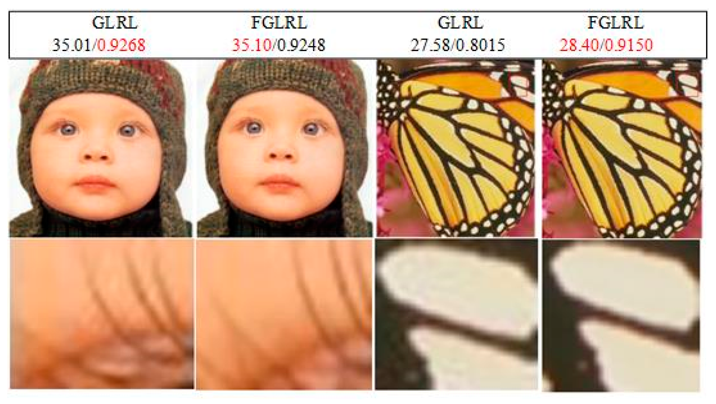
4.3. Discussion of the GLRL and FGLRL

In this paper, before performing non-linear mapping, a shrinking layer is added to compress the feature dimensions. After the mapping, an expanding layer is added to restore the original dimensions, which makes the network structure funnel-shaped. The main purpose is to reduce the number of parameters in the non-linear mapping layer and reduce the computational complexity. This section discusses the effects of the presence and absence of shrinking and expanding layers. We call the network without shrinking and expanding layers of GLRL [16]. Listed in Table 3 are the PSNR and SSIM of GLRL and FGLRL in Set5 and their running time. The reconstruction results of the two methods are compared in Figure 5. It can be seen from Figure 5 and Table 3 that the difference between the reconstruction effect with and without the compression and expansion layer is not large, but the running time with the compression and expansion layer is significantly lower. Without changing the depth of the convolutional network, the running time of the method in this paper is reduced by two to three times.

5. Conclusions

While observing the limitations of current deep learning-based SR models, we explore a more efficient network structure. The inspiration of this network structure mainly comes from the five structures SRCNN, FSRCNN, DRCN, DRRN, and GLRL. This network structure directly convolves the original low-resolution small image, reconstructs it with a deconvolution layer, and adds a shrinking and expanding layer to achieve high operating speed without loss of recovery quality. Extensive experiments show that, compared with other deep neural networks, this method performs better on some datasets in terms of the reconstruction effect, but has a significant reduction in running time and has a satisfactory SR performance.

Author Contributions

Conceptualization, J.H. Methodology, J.H. Software, J.H. Validation, J.H. Formal analysis, J.H. Investigation, X.Y. Resources, X.Y. Data curation, X.Y. Writing—original draft preparation, J.H. Writing—review and editing, Y.S. Supervision, Y.S. Funding acquisition, Y.S. All authors have read and agreed to the published version of the manuscript.

Funding

Science and Technology Development Plan Project of Jilin Province under Grant Nos. 20170414017GH and 20190302035GX, the Natural Science Foundation of Guangdong Province under Grant No. 2016A030313658, the Innovation and Strengthening School Project (provincial key platform and major scientific research project) supported by Guangdong Government under Grant No. 2015KTSCX175, the Premier-Discipline Enhancement Scheme Supported by Zhuhai Government under Grant No. 2015YXXK02-2, and the Premier Key-Discipline Enhancement Scheme Supported by Guangdong Government Funds under Grant No. 2016GDYSZDXK036 supported this work.

Acknowledgments

We are grateful to our anonymous referees for their useful comments and suggestions. The authors also thank Liangliang Li for his useful advice during this work.

Conflicts of Interest

The authors declare no conflict of interest.

References

  1. Thornton, M.W.; Atkinson, P.M.; Holland, D.A. Sub-pixel mapping of rural land cover objects from fine spatial resolution satellite sensor imagery using super-resolution pixel-swapping. Int. J. Remote Sens. 2006, 27, 473–491. [Google Scholar] [CrossRef]
  2. Shi, W.; Caballero, J.; Ledig, C.; Zhuang, X.; Rueckert, D. Cardiac image super-resolution with global correspondence using multi-atlas patch match. Med. Image Comput. Comput. Assist. Interv. 2013, 16, 9–16. [Google Scholar] [PubMed]
  3. Temizel, A.L.P.T.E.K.İ.N.; Vlachos, T.H.E.O. Wavelet domain image resolution enhancement. IEEE Proc. Vis. Image Signal Process. 2006, 153, 25–30. [Google Scholar] [CrossRef]
  4. Yang, J.; Wright, J.; Huang, T.S.; Ma, Y. Image super-resolution via sparse representation. IEEE Trans. Image Process. 2010, 19, 2861–2873. [Google Scholar] [CrossRef] [PubMed]
  5. Lai, W.S.; Huang, J.B.; Ahuja, N.; Yang, M.H. Fast and Accurate Image Super-Resolution with Deep Laplacian Pyramid Networks. IEEE Trans. Pattern Anal. Mach. Intell. 2017, 41, 2599–2613. [Google Scholar] [CrossRef] [PubMed] [Green Version]
  6. Dong, C.; Chen, C.L.; He, K.; Tang, X. Learning a Deep Convolutional Network for Image Super-Resolution. In Proceedings of the Computer Vision, ECCV 2014—13th European Conference, Zurich, Switzerland, 6–12 September 2014; Volume 8692, pp. 184–199. [Google Scholar]
  7. Dong, C.; Chen, C.L.; Tang, X. Accelerating the super-resolution convolutional neural network. In Proceedings of the Computer Vision—14th European Conference, Amsterdam, The Netherlands, 8–16 October 2016; pp. 391–407. [Google Scholar]
  8. Shi, W.; Caballero, J.; Huszár, F.; Totz, J.; Aitken, A.P.; Bishop, R.; Rueckert, D.; Wang, Z. Real-time single image and video super-resolution using an efficient sub-pixel convolutional neural network. In Proceedings of the 2016 IEEE Computer Society Conference on Computer Vision and Pattern Recognition (CVPR), Seattle, WA, USA, 27–30 June 2016; pp. 1874–1883. [Google Scholar]
  9. Kim, J.; Kwon Lee, J.; Mu Lee, K. Accurate Image Super-Resolution Using Very Deep Convolutional Networks. In Proceedings of the 2016 IEEE Computer Society Conference on Computer Vision and Pattern Recognition (CVPR), Seattle, WA, USA, 27–30 June 2016; pp. 1646–1654. [Google Scholar]
  10. Kim, J.; Lee, J.K.; Lee, K.M. Deeply-recursive convolutional network for image super-resolution. In Proceedings of the IEEE Computer Society Conference on Computer Vision and Pattern Recognition (CVPR), Seattle, WA, USA, 27–30 June 2016; pp. 1637–1645. [Google Scholar]
  11. Tai, Y.; Yang, J.; Liu, X. Image super-resolution via deep recursive residual network. In Proceedings of the 30th IEEE/CVF Conference on Computer Vision and Pattern Recognition (CVPR), Honolulu, HI, USA, 21–26 July 2017; pp. 2790–2798. [Google Scholar]
  12. Tong, T.; Li, G.; Liu, X.; Gao, Q. Image Super-Resolution Using Dense Skip Connections. In Proceedings of the 2017 IEEE International Conference on Computer Vision (ICCV) IEEE Computer Society, Venice, Italy, 22–29 October 2017; pp. 4809–4817. [Google Scholar]
  13. Dong, C.; Loy, C.C.; He, K.; Tang, X. Image Super-Resolution Using Deep Convolutional Networks. IEEE Trans. Pattern Anal. Mach. Intell. 2016, 38, 295–307. [Google Scholar] [CrossRef] [PubMed] [Green Version]
  14. Shi, J.; Liu, Q.; Wang, C.; Zhang, Q.; Ying, S.; Xu, H. Super-resolution reconstruction of MR image with a novel residual learning network algorithm. Phys. Med. Biol. 2018, 63, 085011. [Google Scholar] [CrossRef] [PubMed]
  15. He, K.; Zhang, X.; Ren, S.; Sun, J. Deep residual learning for image recognition. In Proceedings of the 2016 IEEE Conference on Computer Vision and Pattern Recognition (CVPR), Seattle, WA, USA, 27–30 June 2016; pp. 770–778. [Google Scholar]
  16. Hou, J.; Si, Y.; Li, L. Image Super-Resolution Reconstruction Method Based on Global and Local Residual Learning. In Proceedings of the 4th International Conference on Image, Vision and Computing, Xiamen, China, 5–7 July 2019. (Accepted). [Google Scholar]
  17. Yang, J.; Wright, J.; Huang, T.; Ma, Y. Image super-resolution as sparse representation of raw image patches. In Proceedings of the IEEE Conference on Computer Vision and Pattern Recognition, Anchorage, AK, USA, 23–28 June 2008; p. 2378. [Google Scholar]
  18. Martin, D.; Fowlkes, C.; Tal, D.; Malik, J. A database of human segmented natural images and its application to evaluating segmentation algorithms and measuring ecological statistics. In Proceedings of the IEEE International Conference on Computer Vision, Vancouver, BC, Canada, 7–14 July 2001; Volume 2, pp. 416–423. [Google Scholar]
  19. Bevilacqua, M.; Roumy, A.; Guillemot, C.; Alberi-Morel, M.L. Low complexity single-image super-resolution based on non-negative neighbor embedding. In Proceedings of the British Machine Vision Conference (BMVC), Surrey, UK, 3–7 September 2012; p. 216. [Google Scholar]
  20. Zeyde, R.; Elad, M.; Protter, M. On single image scale-up using sparse-representations. In International Conference on Curves and Surfaces; Springer: Avignon, France, 24–30 June 2012; pp. 711–730. [Google Scholar]
  21. Huang, J.-B.; Singh, A.; Ahuja, N. Single image superresolution from transformed self-exemplars. In Proceedings of the 2015 IEEE Conference on Computer Vision and Pattern Recognition(CVPR), Boston, MA, USA, 7–12 June 2015; pp. 5197–5206. [Google Scholar]
  22. Timofte, R.; De Smet, V.; Van Gool, L. A+: Adjusted anchored neighborhood regression for fast super-resolution. In Asian Conference on Computer Vision; Springer: Singapore, 1–5 November 2014; pp. 111–126. [Google Scholar]
Figure 1. (a) Super-Resolution Convolutional Neural Network (SRCNN). (b) Accelerating the Super-Resolution Convolutional Neural Network (FSRCNN). (c) Deeply-Recursive Convolutional Network for Image Super-Resolution (DRCN). (d) Image Super-Resolution via Deep Recursive Residual Network (DRRN). (e) Image Super-Resolution Reconstruction Method Based on Global and Local Residual Learning (GLRL).
Applsci 10 01856 g001
Figure 2. The proposed super-resolution image reconstruction framework.
Applsci 10 01856 g002
Figure 3. (a) The partially simplified structure of DRRN. (b) The structure of LRB with a shallow convolutional branch (SCB) and a deep convolutional branch (DCB).
Applsci 10 01856 g003
Figure 4. Qualitative comparison. The first row shows image “img_096” (Urban100 with scale factor ×3). The second row shows image “img_099” (Urban100 with scale factor ×3). The third row shows image “ppt3” (Set14 with scale factor ×4).
Applsci 10 01856 g004
Figure 5. Qualitative comparison. The first image shows “baby” (Set5 with scale factor ×3). The second shows image “butterfly” (Set5 with scale factor ×3).
Applsci 10 01856 g005
Table 1. Comparison of peak signal-to-noise ratio (PSNR) and structural similarity index (SSIM) values for various methods with a scale of ×2, ×3, ×4 on Set5, Set14, Urban100, BSD100.
DatasetScaleBicubicAplusSRCNNVDSRDRCNFGLRL
Set5×233.66/0.929936.55/0.934136.34/0.954237.53/0.958737.63/0.958837.75/0.9633
×330.39/0.868232.59/0.927032.39/0.909033.66/0.921333.82/0.922632.95/0.9105
×428.42/0.810430.28/0.860330.09/0.862831.35/0.883831.53/0.885431.44/0.8846
Set14×230.24/0.868832.28/0.898632.45/0.906733.03/0.912433.04/0.911833.11/0.9133
×327.55/0.774229.13/0.831129.00/0.821529.77/0.831429.76/0.831129.51/0.8325
×426.00/0.702727.33/0.749127.50/0.751328.01/0.767428.02/0.767028.05/0.7688
Urban100×226.88/0.840328.58/0.874429.50/0.894630.76/0.914030.75/0.913329.99/0.9102
×324.46/0.734926.11/0.786926.24/0.798927.14/0.827927.15/0.827627.30/0.8280
×423.14/0.657724.32/0.718324.52/0.722125.18/0.752425.14/0.751025.13/0.7501
BSD100×229.56/0.843130.78/0.876631.36/0.887931.90/0.896031.85/0.894232.30/0.8842
×327.21/0.738528.18/0.764428.41/0.786328.82/0.797628.80/0.796328.66/0.7870
×425.96/0.667526.77/0.708726.90/0.710127.29/0.725127.23/0.723327.26/0.7244
Comment: Red color indicates the best performance of all methods and blue color indicates the second-best performance of all methods.
Table 2. Comparison of average running time of various algorithms.
DatasetBicubicAplusSRCNNVDSRDRCNFGLRL
Set5——0.350.180.740.630.29
Set14——0.690.391.350.980.23
Urban100——0.540.330.890.730.43
BSD100——0.460.230.750.660.32
Comment: Red color indicates the best performance of all methods and blue color indicates the second-best performance of all methods.
Table 3. Comparison of PSNR, SSIM and running time values for GLRL and FGLRL on Set5.
Set5GLRLFGLRL
Baby35.01/0.9268/0.7935.10/0.9248/0.40
Bird37.09/0.9664/0.6835.66/0.9552/0.27
Butterfly27.58/0.8015/0.4328.40/0.9150/0.28
Head33.58/0.8340/0.5733.81/0.8283/0.29
Woman31.33/0.9428/0.6331.76/0.9290/0.25
Comment: Red color indicates the best performance of two methods.

