Multi-Objective Optimization Study of Regenerative Braking Control Strategy for Range-Extended Electric Vehicle

Abstract

Currently, the researches on the regenerative braking system (RBS) of the range-extended electric vehicle (R-EEV) are inadequate, especially on the comparison and analysis of the multi-objective optimization (MOO) problem. Actually, the results of the MOO problem should be mutually independent and balanced. With the aim of guaranteeing comprehensive regenerative braking performance (CRBP), a revised regenerative braking control strategy (RRBCS) is introduced, and a method of the MOO algorithm for RRBCS is proposed to balance the braking performance (BP), regenerative braking loss efficiency (RBLE), and battery capacity loss rate (BCLR). Firstly, the models of the main components related to the RBS of the R-EEV for the calculation of optimization objectives are built in MATLAB/Simulink and AVL/Cruise. The BP, RBLE, and BCLR are selected as the optimization objectives. The non-dominated sorting genetic algorithm (NSGA-II) is applied in RRBCS to solve the MOO problem, and a group of the non-inferior Pareto solution sets are obtained. The simulation results show a clear conflict that three optimization objectives cannot be optimal at the same time. Then, we evaluate the performance of the proposed method by taking the individual with the optimal CRBP as the final optimal solution. The comparation among BP, RBLE, BCLR, and CRBP before and after optimization are analyzed and discussed. The results illustrate that characteristic parameters of RRBCS is crucial to optimization objectives. After parameters optimization, regenerative braking torque works early to increase braking energy recovery on low tire-road adhesion condition, and to reduce the battery capacity loss rate at the expense of small braking energy recovery on the medium tire-road adhesion condition. In addition, the results of the sensitivity analysis show that after parameter optimization, RRBCS is proved to perform better road adaptability regarding the distribution of solutions. These results thoroughly validate the proposed approach for multi-objective optimization of RRBCS and have a strong directive to optimize the control strategy parameters of RBS.

1. Introduction

The range-extended electric vehicle (R-EEV) can greatly improve its driving range through the auxiliary power unit, so as to solve the range anxiety from consumers. As one of the main working modes, the energy recovered with regenerative braking system (RBS) provides an effective approach so as to greatly improve energy efficiency of R-EEV. Research shows that about 20%–50% or more of the driving energy is lost during the braking process [1,2,3,4]. The characteristic parameters of regenerative braking control strategy (RBCS) are crucial to optimization objectives. Thereby, the parameters optimization study on RBCS and the comprehensive regenerative braking performance (CRBP) analysis have gotten a lot of attention and deserve to be studied.

Present research mainly focuses on the balance and optimization between braking performance and braking energy recovery of RBS. Literature [5] focuses on the control algorithm of the braking energy regeneration system of an electric bus in a safety-critical driving situation. A sliding-mode controller based on the exponential reaching law for the antilock braking system is developed in the literature [6]. With the aims of regeneration efficiency and braking safety, three different control strategies are studied in [7,8]. Similar studies are available in the literature [9,10,11,12], which develop the braking torque allocating method to improve braking performance and energy regeneration. In the literature [13], a hierarchical control strategy is proposed, taking battery aging into consideration to ensure vehicle braking safety, recover more energy, and protect components from aging. Cooperative regenerative braking control is proposed in the literature [14] to recover optimal braking energy while guaranteeing the vehicle lateral stability. The longitudinal friction between the road and the tires is estimated and controlled while optimizing regenerative braking in the literature [15]. Moreover, battery is the most sensitive component in the powertrain of R-EEV, so a large regenerative charging current (RCC) can cause damage to the battery and reduce its service life [13].

However, current control strategies pay less attention to the impaction of regenerative braking current (RCC) on the battery state of health and rarely follow this essential characteristic of the multi-objective problem. How to optimize the control parameters of RBCS is mostly derived from the developer’s experience. In addition, how to realize a better balance among the braking performance (BP), regenerative braking loss efficiency (RBLE), and battery capacity loss rate (BCLR) is also studied inadequately. The objective of the regenerative braking control strategy for an R-EEV is to guarantee the comprehensive performance of the R-EEV during operation, and this comprehensive performance includes braking performance and regenerative braking efficiency. Meanwhile, the strategy ensures RCC is always within the controllable range and battery state of charge (SoC) is close to the pre-set value, which not only protects the battery pack, but also gets the ideal braking comprehensive performance.

In this paper, a revised regenerative braking control strategy (RRBCS) based on the optimal slip ratio (OSR) with the rate and shape of battery RCC considerations is introduced. In addition, a multi-objective parameters optimization method (MOOM) for RRBCS is proposed to match the BP, RBLE, and BCLR in the power system of R-EEV. The major contribution and innovations of this work are mainly reflected in the following three aspects: (1) It adds the analysis of RCC’s impact on battery health, and the adverse effects of RCC on battery health are reduced by the designed “conservative braking mode” in RRBCS. (2) The conflict among BP, RBLE, and BCLR are revealed and analyzed through the proposed MOOM, and the control parameters’ optimal solution of RBCS is obtained based on the global optimization algorithm instead of deriving from the developer’s experience to get a better balance among three objectives. (3) The sensitivity analysis of the optimal solution on various tire-road adhesion conditions is carried out to validate the effectiveness and feasibility of the proposed MOOM.

The rest of this paper is organized as follows: In Section 2, the RRBCS is given and revised allocation logic of the regenerative braking work-point is introduced. Section 3 describes the MOO problem, and the non-dominated sorting genetic algorithm (NSGA-II) is selected to solve the MOO problem and simulation model is built. In addition, the simulation test and non-inferior Pareto solution sets are given. In Section 4, a series of simulation tests on various tire-road adhesion conditions are carried out to validate the effectiveness and feasibility of the proposed MOOM. This is followed by the conclusion in the final section.

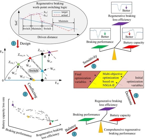
2. Design of the Revised Braking Regenerative Control Strategy

2.1. Process of the Regenerative Braking Control Strategy

A medium R-EEV driven by the front axle was used in this study to design RBCS. As shown in Figure 1, the RBS consists of two systems: the hydraulic braking system and electric braking system. In the hydraulic braking system, the pressure adjustment at the wheel master cylinder can be achieved by modulating valves. Every wheel is equipped with the modulating valves so that each wheel can be controlled by the hydraulic braking controller independently.

The RRBCS studied in this paper was divided into three levels: the highest level (coordinate regenerative braking controller), the second level (fuzzy controller), and the third level (actuator), as shown in Figure 2.

The highest level contains the hydraulic braking controller and the electric controller in RBS, whose main task is to coordinate regenerative braking torque and hydraulic braking torque. The second level contains the double fuzzy logic controller (DFLC), which is different from the fuzzy controller in [16,17,18,19]. Additionally, it can adjust the braking torque in real time to control the slip ratio of the front and rear wheels to achieve a good follow-up of the target slip ratio. The regenerative and hydraulic braking system without a controller is included in the third level, whose task is to realize the braking process under the controller’s supervision.

2.2. Realization of Braking Torque Based on OSR

As shown in Figure 3a, the motor reaches the allowable braking force upper limit T_{mot_max} at point A. The braking strength corresponding to point A is defined as the threshold value of low brake strength Z_{a_l}, and the braking strength corresponding to point B is defined as the threshold value of high brake strength Z_{b_h}. The braking force distribution should follow the ideal braking force distribution curve (I curve), so that the front and rear wheels are locked at the same time to fully use the road surface adhesion. The I curve is related to the vehicle’s actual mass and static axle load, which are variable in daily driving. The ideal braking force distribution is obtained by adjusting the slip ratio of the front and rear wheels. To realize the braking torque control, the relationship between the front and rear axle braking force and the slip ratio is derived as shown in Figure 3b. According to the ECE R13-H braking regulations, the rear wheels must have a certain braking force to maintain vehicle’s stability and braking efficiency when the front and rear wheels are locked. The relationship between the rear wheels’ minimum braking force and the front wheels’ braking force is the M curve, as shown in the Figure 3a.

W is the correction factor with the tire-road adhesion condition consideration. Together with Z_{a_l} and Z_{b_h}, they can be calculated as follows:

$$Z_{a\_l}=\frac{W{T}_{\max \_mot}i}{mgR}$$

(1)

$$Z_{b\_h}=\frac{\sqrt{m_f^2+4Z_{a\_l}{h}_g/l}-m_f}{2h_g/l}$$

(2)

$$\mathrm{W}=\{\begin{array}{l}0,0\le {\mu }_{\max }\le {\mu }_{w\_l}\\ \frac{({\mu }_{\max }-{\mu }_{w\_l})}{({\mu }_{w\_h}-{\mu }_{w\_l})},{\mu }_{w\_l}\le {\mu }_{\max }\le {\mu }_{w\_h}\\ 1,{\mu }_{w\_h}\le {\mu }_{\max }\end{array}$$

(3)

where T_{mot_max} is the motor allowable braking force upper limit; m is the total mass of vehicle; R is the wheelbase; i is the transmission ratio; μ_max is the peak tire-road adhesion coefficient (PTAC); μ_{w_l} is the threshold value of the low tire-road adhesion coefficient (TAC); μ_{w_h} is the threshold value of the high TAC; m_f is the front axle mass distribution coefficient; l is the front and rear axle wheelbase; and h_g is the centroid height.

The distribution values of the slip ratio in three braking stages are described as follows:

(1) Full regenerative braking of the “OA” stage

$$S_f={\phi }_f^{-1}[\frac{Z_{a\_l}}{m_f+Z_{req}{h}_g/l}],S_r=0$$

(4)

(2) Hydraulic braking compensation of the “AB” stage

$$S_f={\phi }_f^{-1}[\frac{Z_{a\_l}}{m_f+Z_{req}{h}_g/l}],S_r={\phi }_r^{-1}[\frac{Z_{req}-Z_{a\_l}}{m_f-Z_{req}{h}_g/l}]$$

(5)

(3) Regenerative braking and hydraulic braking coordination of the “BC” stage

$$S_f={\phi }_f^{-1}[Z_{req}],\begin{array}{c}\end{array}{S}_r={\phi }_r^{-1}[Z_{req}]$$

(6)

Considering the difference of the braking torque between the front and rear wheels, the DFLC for the front and rear wheels is designed to ensure OSR tracking control target values effectively. As shown in Figure 4, the demand slip ratio s_req(t) of the front and rear wheels can be obtained from the demand braking strength calculation and s_osr(t) can be output in real time. If s_req(t) < s_osr(t), the OSR control target s_csr(t) is defined as s_csr(t) = s_req(t). Otherwise, s_csr(t) is defined as s_csr(t) = s_osr(t), and it generally occurs on the low tire-road adhesion condition or the braking strength demand is too large.

There are two inputs in the fuzzy logic controller of the front wheels and the two inputs are the difference between the real slip ratio and the target slip ratio e_f(t), and the slip rate change rate ś_f(t), respectively. The output is the regenerative braking force adjustment value of the front wheel ΔT_{f _e}(t), the hydraulic braking force adjustment value of the front wheel ΔT_{f_m} (t), respectively. There are two inputs in the fuzzy logic controller of the rear wheels and the two inputs are the difference between the real slip ratio and the target slip ratio e_r(t), and the slip rate change rate ś_r(t), respectively. The output is the hydraulic braking force adjustment value of the rear wheel ΔT_{r_m}(t).

2.3. Braking Work-Point Switching Logic of RRBCS

The objective of the regenerative braking control strategy for R-EEV is to guarantee the comprehensive regenerative braking performance during operation. The allocation logic of the braking work-point is crucial to the efficiency of RRBCS [20]. In this paper, the braking work-point in RRBCS was divided into five types, as shown in Figure 5a,b.

Allocation logic of the braking work-point in RRBCS is as follows: (1) If Z_{req_l} < Z_{a_l} and μ_max < μ_{μ_l}, the braking work-point should follow the I curve on work-point 1 (W_C1) to protect the wheel from locking and slipping. (2) If Z_{req_l} < Z_{a_l} and μ_max > μ_{μ_l}, the braking work-point should follow the “OA” curve on work-point 2 (W_C2) to protect the wheel from locking and slipping. Regenerative braking torque provides sufficient braking torque at the front wheel and the rear wheel hydraulic force is 0. (3) If Z_{b_h} > Z_{req_m} > Z_{a_l} and μ_max < μ_{μ_h}, the braking work-point should follow the I curve on work-point 3 (W_C3) to protect the wheel from locking and slipping due to the fact that larger Z_{req_m} exists. (4) If Z_{b_h} > Z_{req_m} > Z_{a_l} and μ_max > μ_{μ_h}, the braking work-point should follow the “AB” curve on work-point 4 (W_C4). The motor will provide its maximum regenerative torque applied at the front wheels, and the insufficient part of the driving braking torque would be compensated by the hydraulic braking system. (5) If Z_{req_h} > Z_{b_h}, the braking work-point should follow the I curve on work-point 5 (W_C5).

In order to control the fluctuation range of the battery SoC and prevent the RCC from being too large to affect the battery life, the regenerative charging work-point of the control logic is referenced in the battery SoC characteristics for conservative adjustments. The strategy makes the SoC close to the pre-set value, which not only protects the battery state of health, but also fully uses the battery pack power. The “conservative braking mode” is a conservative adjustment of the original braking work-point of RBCS. In order to meet the above performance requirements, the braking work-point switching logic needs to be adjusted in real time according to the vehicle status. With SoC characteristics as the switching limit, the braking work-point switching logic is shown in Figure 6.

The battery SoC value at the k instant SoC^(k) and the k + 1 instant SoC^(k+1) were detected, respectively. The SoC change rate k_SoC and change rate discrimination value k_cr were calculated as follows:

$$k_{SoC}=(So{C}^{(k+1)}-So{C}^{(k)})\Delta t^{-1}$$

(7)

$$k_{cr}={\xi }_0{k}_0={\xi }_0(So{C}_0^{(k+1)}-So{C}_0^{(k)})\Delta t^{-1}$$

(8)

where SoC₀ is the SoC control target value; k₀ is the SoC control target change rate on drop stage; the k_{0_CD} is a preset value in charge depletion; the k_{0_CS} = 0 in charge sustaining; and ζ₀ is a correction coefficient with a value of 0.5.

As depicted in Figure 5c and Figure 6, the braking work-point is changed to follow the I curve, that is, W_C1 is switched to W_C2, and the W_C4 is switched to the W_C3. The “conservative braking mode” is realized in three cases and the details are explained as follows: (1) In CD, if k_soc > |k_cr| > 0, the “conservative braking mode” should be used to prevent SoC from deviating too much from SoC₀, which can reduce the adverse impact of RCC on the battery. (2) If 0 > k_SoC > -|k_cr|, the “conservative braking mode” should be adopted to reduce the positive deviation of the SoC₀, because SoC is approaching SoC₀ at a smaller rate. (3) In CS, the SoC is positively deviating from the SoC₀ and the RCC makes the SoC deviation larger. When SoC > 0, the “conservative braking method” should be adopted.

3. Multi-Objective Optimization (MOO) Algorithm for RRBCS of R-EEV

3.1. Description of MOO Problem for RRBCS

Compared with the general optimization problem, any decision variable of the MOO problem may influence any optimization target. Obviously, the essential MOO problem is to solve the mapping relationship of the function. The mapping relationship between the decision space and objective space belongs to a complex many-to-many relationship [21,22]. As we know, the solution set of the multi-objective problem belongs to vector optimization in nature. Among the solution sets, such as the absolute optimal solution, strong efficient solution, fuzzy efficient solution, Pareto optimal solutions, and others, the Pareto optimal solution is the best solution of the multi-objective mapping relation. The Pareto optimal solutions are a set of optimal solutions (Pareto front), among which one cannot be claimed to be better than the other without more information [23,24].

There are many parameters that affect the efficiency of the RRBCS. It is difficult to optimize all parameters due to its complexity and diversity. The vehicle’s structural parameters cannot be changed, but the control parameters of RRBCS can be optimized and changed in reality. From the previous section, the allocation rules of work-point are decided by the four shutdown threshold parameters, namely, μ_{φ_l}, μ_{φ_h}, Z_a-1, and Z_b-h. The tire-road adhesion factor W is a function of μ_{w_l} and μ_{w_h}, which determines the value of Z_a-1 and Z_b-h.

The problem described in this section is optimization with the objective of I_{bp_cyc}, I_{rble_cyc}, I_{bclr_cyc}, and I_{crbp_cyc} under multidimensional constraints. Therefore, the overall expression of the objective is expressed as follows:

$$J_{\min }[{\mu }_{\phi \_l},\begin{array}{c}{\mu }_{\phi \_h},{\mu }_{w\_l},{\mu }_{w\_h}\end{array}]=\arg {\displaystyle {\int }_0^T{\omega }_b{I}_{bp\_cyc}+}{\omega }_r{I}_{r\_cyc}+{\omega }_l{I}_{bclr\_cyc}$$

(9)

In the expression, J_min represents the minimum total evaluation indicator of control system, and μ_{φ_l}, μ_{φ_h}, μ_{w_l}, and μ_{w_h} represent a set of optimization variables that make the objective function obtain its minimum I_{bp_cyc}, I_{rbe_cyc}, and I_{bclr_cyc}, respectively. I_{bp_cyc} represents the evaluation indicator of braking performance, I_{rble_cyc} represents the evaluation indicator of regenerative braking loss efficiency, and I_{bclr_cyc} represents the battery capacity loss rate.

3.2. Optimization Objective Calculation

3.2.1. Braking Performance (BP)

The evaluation indicator of the braking performance I_{bp_cyc} characterizes the agreement between the actual braking strength and the target value, which is a calculation of the mean square error value of the braking strength. I_{bp_cyc} is calculated as follows:

$$I_{bp\_cyc}=\sqrt{\frac{1}{N}{\displaystyle \sum _{i=1}^N{(Z_{act}(t)-Z_{req}(t))}^2}}$$

(10)

where Z_act is the actual braking strength and Z_req is the required braking strength.

3.2.2. Regenerative Braking Loss Efficiency (RBLE)

The MOO problems are described as cost-type optimization problems. It is expected that the objective function values are as small as possible. The evaluation indicator of the regenerative braking efficiency optimization problem is a revenue-type optimization problem. It is expected that the I_{rbe_cyc} is as large as possible.

$$I_{rbe\_cyc}=\frac{E_{regen\_off}-E_{regen\_on}}{E_{regen\_off}}\times 100\%$$

(11)

where E_{regen_on} and E_{regen_off} are the energy consumed with and without RBC under a driving cycle, respectively. I_{rbe_cyc} can be represented as the contribution made by regenerative braking to energy consumption reduction.

In order to construct a cost optimization problem uniformly, the evaluation indicator of regenerative braking loss efficiency I_{rble_cyc} is calculated as follows:

$$I_{rble\_cyc}=1-I_{rbe\_cyc}$$

(12)

I_{rble_cyc} essentially represents the proportion of regenerative braking energy that is not recovered during the braking process.

3.2.3. Battery Capacity Loss Rate (BCLR)

Charging current profiles can be changed and controlled to obtain the optimal charging capacity without affecting the battery service life [25]. The battery is subjected to repeated operations of charging and discharging profiles, and the rate and shape of the charging current undoubtedly affect the BCLR. Battery current I(t) and life cycles N_cyc are selected as model reference variables in the battery capacity loss model (BCLM) referred to [26,27]. According to the measurements of battery capacity fading in [25], battery capacity loss rate I_{bclr_cyc} and the capacity attenuation coefficient α₁ can be calculated as follows:

$$I_{bclr\_cyc}={\alpha }_1\times N_{cyc}\times DOD\times A{h}_{cell}$$

(13)

$${\alpha }_1=B_1\times \exp (B_2{C}_n)=B_1\times \exp (B_2\frac{I(t)}{A{h}_{cell}})$$

(14)

where DOD is the depth of discharge; Ah_cell is the cumulative capacity of the battery; C_n is the charging rate; and I(t) is the battery current.

B₁ and B₂ is the fitting parameter, which can be calculated through the least squares method. Under comprehensive driving cycle conditions, the BCLM can be obtained as follows:

$$I_{bclr\_cyc}={\displaystyle {\int }_0^{T_{cyc}}{B}_1\times B_2\times }{I}^{\prime }(t)\times \exp (B_2\frac{I(t)}{A{h}_{cell}})\times N_{cyc}\times DODdt$$

(15)

where T_cyc is the total cycle time.

Considering that the focus of this research is on the application of the BCLM and article length limitation, a reference can be made in [25,26,27,28] for the experimental details of the battery life cycle. By fitting the experimental data, the following can be acquired: B₁ = 0.0018 and B₂ = 0.3785.

3.3. Optimization Decision Based on the Comprehensive Regenerative Braking Performance (CRBP)

A well-distributed Pareto optimal solution set is found through the optimization algorithm. In engineering practice, only one final solution is needed. So, just finding the Pareto optimal solution set does not completely solve the MOO problem. The multi-objective normalization optimization discussed in this paper adopts the linear normalization method, which is simple, practical, and efficient to deal with the frontier of non-convex problems. Additionally, it can reflect the weights of optimization goals clearly. Since the above four optimization variables represent different physical meanings, it is necessary to unify the cost functions in each dimension by normalizing the normalization method. After transformation, it becomes a dimensionless expression.

Normalization of linear functions (Min–Max scaling) converts the original data linearization method to the range of [0, 1]. The normalization formula is as follows:

$$X^{(nor)}=\frac{X_p-X_p^{(\min )}}{X_p^{(\max )}-X_p^{(\min )}}$$

(16)

where X^(nor) is the normalized data; X_p is the original data in Pareto optimal solution sets; and X_p^(nax) and X_p^(min) are the maximum and minimum values of the original data sets respectively.

The evaluation indicator of comprehensive regenerative braking performance I_{crbp_cyc} is calculated as follows:

$$I_{crbp\_cyc}={\lambda }_b{I}_{bp\_cyc}^{(nor)}+{\lambda }_r{I}_{rble\_cyc}^{(nor)}+{\lambda }_l{I}_{bclr\_cyc}^{(nor)}$$

(17)

where λ is the weighting coefficients of normalized data.

Different weighting results are obtained when different weighting coefficients are selected. Designers can choose a reasonable weight coefficient allocation based on design performance requirements. In this paper, the weight parameter selection is as follows: [λ_b, λ_r, λ_l] ^T = [0.4, 0.3, 0.3] ^T.

4. Simulation and Result Discussion of the MOO Problem

4.1. Non-Dominated Sorting Genetic Algorithm (NSGA-II)

For the MOO problem, it is difficult to directly judge the merits and demerits of the individual. It needs a comprehensive index to evaluate all objectives. NSGA-II is a kind of multi-objective evolutionary algorithm based on Pareto-optimal solutions to solve the MOO problem, which has conflicting objectives. NSGA-II can build solution sets with fast non-dominated sorting and the crowd distance computing method, which is an adaptive global optimization algorithm and has better performance such as a faster convergence speed, better convergence effect, better robustness, and adaptive ability. It assures a good convergence towards the Pareto-optimal front without losing the solution diversity [29]. A detailed explanation and steps of NSGA-II can be found in [30]. In this study, the population size of the algorithm was set to be 200, and the number of generations was set to be 100. The flowchart for implementing the algorithm in solving the MOO problem is shown in Figure 7.

In the present work, according to the characteristics of optimization variables, binary cross mutations are simulated by real number encoding. The algorithm mutation can be adjusted adaptively to improve the global search ability in the early stage and local search ability in the later stage. Meanwhile, in order to increase the convergence speed and ensure the global optimality of the Pareto solution set, the process of simulating the binary cross mutation of the algorithm is as follows:

$$\{\begin{array}{l}{x}_i^{(k+1)}=c_i(\lambda )x_i^{(k)}+(1-c_i(\lambda ))x_{i+1}^{(k)}\\ x_{i+1}^{(k+1)}=c_i(\lambda )x_{i+1}^{(k)}+(1-c_i(\lambda ))x_i^{(k)}\\ x_j^{(k+1)}=(1+c_j(\lambda ))x_j^{(k)}\end{array}$$

(18)

where x_i^(k+1) and x_i+1^(k+1) are the individuals before crossing; x_i^(k) and x_i+1^(k) are the individuals after crossing; k is the evolutionary algebra; c_i(λ) is the cross coefficient, using the dynamic state adjustment mechanism; x_j^(k) is the individual to be mutated; and c_j(λ) is the coefficient of variation.

It is necessary to make corresponding changes in c_i(λ) and c_j(λ) to maximize the performance of the algorithm according to the change of the solution set. The algorithm is further improved so that c_i(λ) and c_j(λ) can adapt to the changes of the solution set. The adaptive change model is expressed as:

$$\{\begin{array}{l}\lambda =N_p/N_a\\ c_i(\lambda )=\frac{1}{2}{e}^{\lambda }\\ c_j(\lambda )=e^{\lambda }\end{array}$$

(19)

where λ is the adaptive coefficient of variation; N is the number of populations; and N_p is the optimal number of solutions.

4.2. Simulation Analysis of NSGA-II

MOO Simulation Model

In order to guarantee the Pareto solution sets and evaluate the control effect of the strategies during deceleration braking, several simulations experiments were carried out to verify the feasibility and effectiveness of the system in MATLAB/Simulink and AVL-Cruise software. The main parameters used in the simulations are shown in

Table 1. Parameters of the multi-objective optimization (MOO) simulation model.

Parameter	Value	Parameter	Value
Full load weight (kg)	1700	Battery capacity (kWh)	20
Wheelbase (mm)	2865	Initial SoC (state of charge)	0.8
Distance from front axle to centroid (mm)	1352	Diameter of front wheel cylinder (mm)	56.95
Distance from rear axle to centroid (mm)	1513	Diameter of rear wheel cylinder (mm)	33.82
Centroid height (mm)	500	Diameter of master cylinder (mm)	18
Drag area (m2)	1.66	Effective radius of front brake rotor (mm)	0.235
Correction coefficient of rotating mass	1.1	Effective radius of rear brake rotor (mm)	0.227
Mechanical efficiency	0.96	Brake pedal leverage ratio	3.5
Transmission reduction ratio	4.2	Diameter of pedal travel simulator (mm)	15

.

The API function provided by the Cruise software was used to develop vehicle control strategy on Simulink, while vehicle model development and the simulation calculation for vehicle performance were conducted on the Cruise. The vehicle control strategy was developed by the means of Simulink and the API function was provided by the Cruise. Vehicle model development and simulation calculations of vehicle performance are carried out on Cruise. The signals data such as traction and breaking, battery SoC, and V_veh were transferred via the interface of Cruise to Simulink. The analysis results were sent back to Cruise via the interface. Simulation on the power system was conducted in the Cruise model.

In the model, the values of the output form a vector by a multiplexer. After completing the simulation step successfully, the output vector was transferred into the Matlab Workspace by the Matlab object “Block Parameters: To Workspace,” and Cruise could access it. The output values of the model had to be combined to a vector. Cruise got this vector and put its elements onto the data bus where they could be used by other components. The vehicle’s dynamic model and regenerative braking control system were established in Cruise and Simulink, respectively, using a co-simulation model as seen in Figure 8.

In order to verify the effectiveness of MOO algorithm, a co-simulation test was carried out based on the braking system model of R-EEV in the simulation environment. A customized typical deceleration braking (CTDB) was defined, as shown in Figure 9a. In simulations, the initial braking speed was set at 80 km/h. The braking strength increased slowly from 0 to 0.2 in 2 s and then increased quickly to 0.7 to simulate emergency braking conditions, and finally it stabilized at 0.5 until the vehicle speed was 0. A comprehensive driving cycle consisting of the CTDB, New European Drive Cycle (NEDC), China Light-duty Vehicle Test Cycle (CLTC), and World Light vehicle Test Procedure (WLTP) was set up, as shown in Figure 9b.

Three different roads were assumed, namely, a dry asphalt surface with a high PTAC (μ_max__h = 0.9), dry cement surface with a medium PTAC (μ_max__m = 0.6), and wet cobblestone surface with a low PTAC (μ_max__l = 0.3), respectively.

4.3. Results Analysis Based on Pareto Solution Sets

As we know, the theory of Pareto optimality can reflect the essential characteristic of the MOO problem better. Therefore, the evolutionary algorithm based on the Pareto principle is proposed to solve the MOO problem. The existence of the optimal solution sets was further studied, and a group of non-inferior Pareto solution sets was obtained. The conflicting relationship among the three objectives is shown in Figure 10. The four evaluation indexes of BP, RBLE, BCLR, and CRBP were comparatively analyzed.

The optimization results are summarized in

Table 2. Optimization results.

Item (High Adhesion)	Solution 1 (Best BP)	Solution 2 (Lowest RBLE)	Solution 3 (Lowest BCLR)	Solution 4 (Best CRBP)
[μφ_l, μφ_h, μw_l, μw_h]	[0.17, 0.51, 0.44, 0.77]	[0.21, 0.48, 0.24, 0.49]	[0.22, 0.62, 0.29, 0.78]	[0.18,0.53, 0.29, 0.66]
Ibp_cyc (m/s2)	0.0407	0.0473	0.0409	0.0421
Irble_cyc	0.76	0.68	0.73	0.72
Ibclr_cyc (%)	2.9	11.7	2.3	4.7
Icrbp_cyc	0.61	0.55	0.66	0.83
Item (Medium adhesion)	Solution 1 (Best BP)	Solution 2 (Lowest RBLE)	Solution 3 (Lowest BCLR)	Solution 4 (Best CRBP)
[μφ_l, μφ_h, μw_l, μw_h]	[0.15, 0.58, 0.43, 0.75]	[0.23, 0.47, 0.22, 0.47]	[0.21, 0.60, 0.28, 0.78]	[0.12,0.54, 0.28, 0.66]
Ibp_cyc (m/s2)	0.0411	0.0475	0.0415	0.0426
Irble_cyc	0.76	0.69	0.75	0.73
Ibclr_cyc (%)	3.1	12.3	2.8	4.8
Icrbp_cyc	0.60	0.54	0.63	0.81
Item (Low adhesion)	Solution 1 (Best BP)	Solution 2 (Lowest RBLE)	Solution 3 (Lowest BCLR)	Solution 4 (Best CRBP)
[μφ_l, μφ_h, μw_l, μw_h]	[0.05, 0.58, 0.41, 0.72]	[0.03, 0.44, 0.22, 0.47]	[0.11, 0.61, 0.26, 0.78]	[0.05,0.53, 0.27, 0.64]
Ibp_cyc (m/s2)	0.0415	0.0476	0.0428	0.0432
Irble_cyc	0.78	0.70	0.77	0.75
Ibclr_cyc (%)	3.6	12.4	4.1	4.9
Icrbp_cyc	0.58	0.51	0.62	0.77

.

The results of the experiment on the high tire-road adhesion condition were taken as an example for discussion and analysis. As shown in

Table 3. Results of the variables.

Item	Optimization Variables				Evaluation Indexes
	μφ_l	μφ_h	μw_l	μw_h	Ibp_cyc	Irble_cyc	Ibclr_cyc	Icrbp_cyc
First generation	0.20	0.40	0.40	0.60	0.443	79.4%	16.1%	0.32
Last generation	0.10	0.53	0.28	0.65	0.428	75.1%	11.2%	0.71

and Figure 10, the conflict was reflected as the following aspects: (1) Under the best BP (S1), I_{bp_cyc} = 0.0407 with a best braking performance, I_{bclr_cyc} = 2.9 with a better battery state of health (SOH). However, I_{rble_cyc} = 0.76 with the worst braking recovery efficiency. The worse I_{crbp_cyc} = 0.61 was caused by the worst indicator I_{rble_cyc}. A similar situation manifested under the lowest BCLR (S3). (2) Under the lowest RBLE (S2), I_{rble_cyc} = 0.68 with the best braking recovery efficiency. However, I_{bp_cyc} = 0.0473 with the worst braking performance and I_{bclr_cyc} = 11.7 with the worst battery SOH, which caused the worst I_{crbp_cyc}. (3) Under the best CRBP (S4), although none of the three indicators were optimal, they were suboptimal and made the best I_{crbp_cyc.} The performance optimization of one single target may inevitably damage the other targets. The optimization results should be multiple sets of solutions rather than a single optimal solution. Each point represents a set of alternatives. BP, RBLE, and BCLR present a clear conflict, and three optimization objectives cannot be optimal at the same time. Since reducing regenerative braking efficiency tends to extend the battery life, the battery RCC is limited to the maximum. The braking work-point on high regenerative braking will switch to low regenerative braking on the I curve to ensure braking performance better, which means the high braking performance reduces the regenerative braking efficiency to a certain extent and causes the conflict.

The above obtained Pareto optimal solution sets consist of a series of discrete points. It needs only one index to show optimal values and evaluation index more clearly. Therefore, averaging method is adopted to fit the discrete optimal points into optimal value. The averaging Pareto optimal solution set is calculated as follows:

$$X^{(k)}=\frac{1}{3N}{\displaystyle \sum _{m=1}^3{\displaystyle \sum _{n=1}^N{x}_n^{(k)}(\mu (m))}}$$

(20)

$$Y^{(k)}=\frac{1}{3N}{\displaystyle \sum _{m=1}^3{\displaystyle \sum _{n=1}^N{y}_n^{(k)}(\mu (m))}}$$

(21)

where x_n^(k) is the optimal solution set in the k-th generation; X^(k) is the averaging value of optimal solution set in the k-th generation; y_n^(k) is the evaluation indicator in the k-th generation; and Y^(k) is the averaging value of evaluation indicator in the k-th generation.

When the optimization range contains all regions, all solution sets can be represented by their respective averages. It should be emphasized that the results of average values were not the real optimal solution under CRBP. However, we could understand and observe the optimal solution set through the trend during each iteration. The optimization calculation results are shown in Figure 11 and Table 3.

It can be seen clearly that optimization variables converged to a stable value after about 60 optimization iterations eventually. Additionally, the convergence trajectories of optimization variables during iteration show some difference. Four optimization variables could converge to the stable Pareto solution sets, which reflect that the MOOM for RRBCS proposed in this paper could achieve the Pareto solution sets “regional convergence” of the MOO problem. “Regional convergence” can be understood as a process, which refers that optimal individual in the Pareto solution sets flows to the Pareto front during the iteration. In addition, four evaluation indexes converged towards the optimization direction. I_{bp_cyc} reduced from the initial value of 0.443–0.428, a decrease of about 3.4%. I_{rble_cyc} reduced from the initial value of 79.4%–75.1%, a decrease of about 5.4%. I_{bclr_cyc} reduced from the initial value of 16.1%–11.2%, a decrease of about 30.4%. I_{bp_cyc} increased from the initial value of 0.32–0.71, an increase of 0.39. The results prove the effectiveness and feasibility of the MOOM.

4.4. Optimization Decisions and Results Discussion

Taking the individual with comprehensive regenerative braking performance as the final optimization solution, the optimal variable solution was [μ_{φ_l}, μ_{φ_h}, μ_{w_l}, μ_{w_h}]^T = [0.11, 0.53, 0.28, 0.65]^T. The results of the brake strength thresholds Z_a-l and Z_b-h after optimization are summarized in

Table 4. Results of Z_a-l and Z_b-h after optimization.

Parameter Za_l	High Adhesion	Medium Adhesion	Low Adhesion
Before optimization	0.400	0.400	0.0000
After optimization	0.400	0.346	0.0757
Parameter Zb_h	High adhesion	Medium adhesion	Low adhesion
Before optimization	0.600	0.400	0.0000
After optimization	0.600	0.533	0.1318

.

As shown in Figure 12, the points with “ ⃰ ” represent the regenerative braking work-point after optimization, and the points without “ ⃰ ” represent the regenerative braking work-point before optimization. It can be seen that Z_a-l and Z_b-h at points A and B remain unchanged before and after optimization on high TAC. After optimization, points A and B move forward to A⃰ and B⃰ on medium TAC and points A and B move backward to A⃰ and B⃰ on low TAC.

In addition, changes of the W function before and after optimization is shown in Figure 13.

The analysis of the simulation results is described as follows: (1) In the case of μ_max ∈ (0, μ⃰_{w_l}] = (0, 0.28], the wheel had a risk of slipping due to the poor TAC. The control parameters and W function did not change after optimization (W⃰ = W = 0), the braking work-points were on the I curve to ensure the braking safety, and the front and rear wheel braking torques were provided by hydraulic torque. (2) In the case of μ_max ∈ (μ⃰_{w_l}, μ_{w_l}] = (0.28, 0.4], the threshold value μ_{w_l} “drill down” after optimization (W⃰ > W), which made the regenerative braking torque “enter ahead” to increase the regenerative braking energy. As shown in Figure 12a, under the conditions of low PTAC, the braking work-points C(W_c5) and D(W_c5) on the I curve before optimization would switch to C*(W_c1) and D*(W_c3) after optimization. (3) In the case of μ_max ∈ (μ_{w_l}, μ_{w_cr}] = (0.4, 0.54], threshold switching points A and B moved backward after optimization, and the regenerative braking ratio did not change or became larger at the same braking strength. (4) In the case of μ_max ∈ (μ_{w_cr}, μ⃰_{w_h}] = (0.54, 0.65], the threshold value μ_{w_h} “goes up” after optimization (W⃰ < W), which accompanied by the threshold switching points A and B moved forward after optimization. Under the demand of high braking strength, the risk of locking and slipping was prone to occur. It can “sacrifice” smaller braking energy in exchange for better braking performance to ensure braking safety after parameter optimization. As shown in Figure 12b, under the demand of low braking strength, the braking work-points E(W_c1) before optimization would switch to E*(W_c4) after optimization, and under the demand of medium braking strength, the braking work-points G(W_c4) and I(W_c4) before optimization would switch to G*(W_c4) and I*(W_c5) after optimization. (5) In the case of μ_max ∈ (μ⃰_{w_h}, 1) = (0.65, 1), the threshold switching points A and B remained unchanged after optimization (W⃰ = W = 1), as shown in Figure 12c.

In summary, in the case of low TAC, the parameters could be optimized to make the regenerative braking starting threshold “drill down”; in the case of medium TAC, the optimization direction focused more on energy recovery while ensuring braking safety; in the case of high TAC and high-strength braking, RRRBCS would “sacrifice” smaller regenerative braking energy in exchange for better braking performance.

5. Discussion and Sensitivity Analysis of RRBCS Based on the Optimization Results

From the above discussion, it could be seen clearly that on the three different tire-road adhesion condition, the influence of control parameters on the performance of RRBCS was different. Therefore, simulation tests were designed to analyze the sensitivity of the different tire-road condition to optimization objective functions. The simulation results of three driving cycles were statistically analyzed, as shown in Figure 14, Figure 15 and Figure 16.

As depicted in Figure 14, when the PTAC was in the range of 0–0.35 and 0.55–1.0, I_{bp_cyc} were similar and close before and after parameters optimization. There was a significant difference before and after optimization when the PTAC was in the range of 0.35–0.55. Compared with the braking process controlled by RRBCS before parameters optimization, I_{bp_cyc} decreased significantly and ∆I_{bp_cyc} was up to about 7% when μ_max = 0.38. In addition, the performance result of recovery energy was similar to BP. As depicted in Figure 15, when the adhesion coefficient was in the range of 0.35–0.5, the recovery braking energy controlled by the proposed control strategy after parameters optimization was about 26.71%. Compared with the braking process controlled by RRBCS before parameters optimization, the recovery braking energy could improve 19.3% after parameters optimization, which denotes that the RRBCS was effective to improve the regenerative energy after parameters optimization.

As depicted in Figure 16, when the tire-road adhesion coefficient was in the range of 0.2-0.5, after parameters optimization, I_{bclr_cyc} reduced slightly and ∆I_{bclr_cyc} was up to about 1.2% when μ_max = 0.52. When the adhesion coefficient was in the range of 0.55–0.75, ∆I_{bclr_cyc} decreased significantly and ∆I_{bclr_cyc} was up to about 5.3% when μ_max = 0.63, which denotes that the RRBCS was effective to reduce the battery capacity loss rate after parameters optimization.

The optimization calculation results are shown in

Table 5. Results of optimization.

Item	Ibp_cyc			Irble_cyc			Ibclr_cyc
	WLTP	NEDC	CLTC	WLTP	NEDC	CLTC	WLTP	NEDC	CLTC
μmax	0.38	0.38	0.38	0.42	0.42	0.42	0.64	0.62	0.62
∆Imax (%)	−4.7	−7.1	−5.9	−16.1	−19.3	−18.4	−4.9	−4.8	−4.8

.

As shown in Table 5, after parameters optimization, I_{bp_cyc} reduced about 4.7%–7.1% when μ_max = 0.38, I_{rble_cyc} reduced about 16.1%–19.3% when μ_max = 0.42, and I_{bclr_cyc} reduced about 4.8% when μ_max = 0.62. As a comparison, the results of this optimal response to different tire-road conditions reflected different performances, which means that the sensitivity of optimization parameters to different road conditions was different. This is due to three main reasons: first, the vehicle’s safety is the main factor in the emergency situation, and the optimization direction is more focused on ensuring braking safety, especially on low and medium tire-road adhesion conditions; second, the regenerative braking torque will “enter ahead” to increase the regenerative braking energy while ensuring braking safety; and third, regenerative braking torque participates in energy recovery in advance, which causes increased recovery current from zero. Overall RRBCS was robust to change on the road conditions and the effectiveness of the proposed strategy could be verified by tests.

6. Conclusions

In this paper, a multi-objective optimization system with various conflicting objectives and a parameters optimization method of RRBCS were proposed to design an optimal RBCS for R-EEV. The method consists of the following steps: (1) A RRBCS was proposed and used in simulation to balance BP, RBLE, and BCLR. (2) The MOO model was established to calculate the objective functions by using simulation results of RRBCS on three different tire-road adhesion conditions. (3) The individual with optimal CRBP was selected as the final optimization solution to evaluate the performance of the proposed methodology, and control parameters decision and optimization results were analyzed and discussed. (4) A study on the sensitivity of the different PTAC to three optimization objectives was conducted through a series of simulation tests.

The reasonable parameter optimization of RRBCS enabled the RBS work to become more efficient and to balance the BP, RBLE, and BCLR. The results analysis based on Pareto solution sets show that BP, RBLE, and BCLR presented a clear conflict, and three optimization objectives could not reach the optimal at the same time. The “regional convergence” of variables could also prove the effectiveness and feasibility of MOOM by statistical analysis. Under the final optimization solution [μ_{φ_l}, μ_{φ_h}, μ_{w_l}, μ_{w_h}]^T = [0.11, 0.53, 0.28, 0.65] ^T, optimized threshold parameters μ_{w_l} and μ_{w_h} show a bipolar expansion to make regenerative braking torque work early to increase regenerative braking efficiency on low tire-road adhesion condition, and reduce the battery capacity loss rate at the expense of small braking energy recovery on medium tire-road adhesion condition. The influence of final optimization control parameters on evaluation indexes on different tire-road adhesion condition was discussed and analyzed, and a more detailed discussion was in the subsequent sensitivity analysis. RRBCS was proved to perform better road adaptability regarding the distribution of solutions. Under the medium and low tire-road adhesion condition, the improvement obtained by optimization was the most significant. This study could provide more references for the optimal control strategy and laid a foundation for multi-objective regenerative braking energy control of the actual vehicle.

References

1. Du, J.; Ouyang, D. Progress of Chinese electric vehicles industrialization in 2015: A review. Appl. Energy 2016, 188, 529–546. [Google Scholar] [CrossRef]
2. Chen, B.; Wu, Y.; Tsai, H. Design and analysis of power management strategy for range extended electric vehicle using dynamic programming. Appl. Energy 2014, 113, 1764–1774. [Google Scholar] [CrossRef]
3. Ma, H.; Balthasar, F.; Tait, N.; Riera-Palou, X.; Harrison, A. A new comparison between the life cycle greenhouse gas emissions of battery electric vehicles and internal combustion vehicles. Energy Policy. 2012, 44, 160–173. [Google Scholar] [CrossRef]
4. Qiu, C.; Wang, G. New evaluation methodology of regenerative braking contribution to energy efficiency improvement of electric vehicles. Energy Convers. Manag. 2016, 119, 389–398. [Google Scholar] [CrossRef]
5. Lv, C.; Zhang, J.; Li, Y.; Yuan, Y. Novel control algorithm of braking energy regeneration system for an electric vehicle during safety–critical driving maneuvers. Energy Convers. Manag. 2015, 106, 520–529. [Google Scholar] [CrossRef]
6. Guo, J.; Jian, X.; Lin, G. Performance evaluation of an anti-lock braking system for electric vehicle with a fuzzy sliding mode controller. Energies 2014, 7, 6459–6476. [Google Scholar] [CrossRef] [Green Version]
7. Kumar, C.N.; Subramanian, S.C. Cooperative control of regenerative braking and friction braking for a hybrid electric vehicle. Proc. Inst. Mech. Eng. J. Automob. Eng. 2015, 230, 103–116. [Google Scholar] [CrossRef]
8. Zhang, J.; Lv, C.; Gou, J.; Kong, D. Cooperative control of regenerative braking and hydraulic braking of an electrified passenger car. J. Automob. Eng. 2012, 226, 1289–1302. [Google Scholar] [CrossRef]
9. Qiu, C.; Wang, G.; Meng, M.; Shen, Y. A novel control strategy of regenerative braking system for electric vehicles under safety critical driving situations. Energy 2018, 149, 329–340. [Google Scholar] [CrossRef]
10. Yin, G.; Jin, X. Cooperative Control of Regenerative Braking and Antilock Braking for a Hybrid Electric Vehicle. Math. Probl. Eng. 2013, 4, 1–9. [Google Scholar] [CrossRef] [Green Version]
11. Wei, Z.; Xu, J.; Halim, D. Braking force control strategy for electric vehicles with load variation and wheel slip considerations. IET Electr. Syst. Transp. 2017, 7, 41–47. [Google Scholar] [CrossRef]
12. Li, L.; Zhang, Y.; Yang, C. Model predictive control-based efficient energy recovery control strategy for regenerative braking system of hybrid electric bus. Energy Convers. Manag. 2016, 111, 299–314. [Google Scholar] [CrossRef]
13. Wu, J.; Wang, X.; Li, L.; Qin, C.; Du, Y. Hierarchical control strategy with battery aging consideration for hybrid electric vehicle regenerative braking control. Energy 2018, 145, 301–312. [Google Scholar] [CrossRef]
14. Han, J.; Park, Y.; Park, Y. Cooperative regenerative braking control for front-wheel-drive hybrid electric vehicle based on adaptive regenerative brake torque optimization using under-steer index. Int. J. Automot. Technol. 2014, 15, 989–1000. [Google Scholar] [CrossRef]
15. Le Solliec, G.; Chasse, A.; Geamanu, M. Regenerative braking optimization and wheel slip control for a vehicle with in-wheel motors. IFAC Proc. Vol. 2013, 46, 542–547. [Google Scholar] [CrossRef]
16. Roumila, Z.; Rekioua, D.; Rekioua, T. Energy management based fuzzy logic controller of hybrid system wind/photovoltaic/diesel with storage battery. Int. J. Hydrog. Energy 2017, 42, 19525–19535. [Google Scholar] [CrossRef]
17. Aksjonov, A.; Vodovozov, V.; Augsburg, K.; Petlenkov, E. Design of regenerative anti-lock braking system controller for 4 in-wheel-motor drive electric vehicle with road surface estimation. Int. J. Automot. Technol. 2018, 19, 727–742. [Google Scholar] [CrossRef] [Green Version]
18. Maia, R.; Silva, M.; Araújo, R.; Nunes, U. Electrical vehicle modeling: A fuzzy logic model for regenerative braking. Expert Syst. Appl. 2015, 42, 8504–8519. [Google Scholar] [CrossRef]
19. Topalov, A.V.; Oniz, Y.; Kayacan, E.; Kaynak, O. Neuro-fuzzy control of antilock braking system using sliding mode incremental learning algorithm. Neurocomputing 2011, 74, 1883–1893. [Google Scholar] [CrossRef]
20. Xu, G.; Xu, K.; Zheng, C.; Zhang, X.; Zahid, T. Fully electrified regenerative braking control for deep energy recovery and maintaining safety of electric vehicles. IEEE Trans. Veh. Technol. 2016, 65, 1186–1198. [Google Scholar] [CrossRef]
21. Shashi, A.; Wang, G.; An, Q. Using the Pareto set pursuing multi-objective optimization approach for hybridization of a plug-in hybrid electric vehicle. J. Mech. Des. 2012, 134, 503–509. [Google Scholar]
22. Yang, G.; Li, S.; Qu, J. Multi-objective optimization of hybrid electrical vehicle based on Pareto optimality. J. Shanghai Jiaotong Univ. 2012, 46, 1297–1303. [Google Scholar]
23. Yang, G.; Zhang, A.; Li, S.; Wang, Y.; Wang, Y.; Xie, Q. Multi-objective evolutionary algorithm based on decision space partition and its application in hybrid power system optimization. Appl. Intell. 2017, 46, 827–844. [Google Scholar] [CrossRef]
24. Nandi, A.K.; Chakraborty, D.; Vaz, W. Design of a comfortable optimal driving strategy for electric vehicles using multi-objective optimization. J. Power Sources 2015, 283, 1–18. [Google Scholar] [CrossRef]
25. Li, J.; Jin, X.; Xiong, R. Multi-objective optimization study of energy management strategy and economic analysis for a range-extended electric bus. Energy Policy. 2017, 194, 798–807. [Google Scholar] [CrossRef]
26. Jiang, Y.; Jiang, J.; Zhang, C.; Zhang, W.; Gao, Y.; Guo, Q. Recognition of battery aging variations for LiFePO4 batteries in 2nd use applications combining incremental capacity analysis and statistical approaches. J. Power Sources 2017, 360, 180–188. [Google Scholar] [CrossRef]
27. Wang, J.; Purewal, J.; Liu, P.; Hicks-Garner, J.; Soukazian, S.; Sherman, E. Degradation of lithium ion batteries employing graphite negatives and nickel–cobalt–manganese oxide+ spinel manganese oxide positives: Part 1, aging mechanisms and life estimation. J. Power Sources 2014, 269, 937–948. [Google Scholar] [CrossRef]
28. Abdel-Monem, M.; Trad, K.; Omar, N.; Hegazy, O.; Peter, V.D.B.; Van Mierlo, J. Influence analysis of static and dynamic fast-charging current profiles on ageing performance of commercial lithium-ion batteries. Energy 2017, 120, 179–191. [Google Scholar] [CrossRef]
29. Kamjoo, A.; Maheri, A.; Dizqah, A.M.; Putrus, G.A. Multi-objective design under uncertainties of hybrid renewable energy system using NSGA-II and chance constrained programming. Int. J. Electr. Power Energy Syst. 2016, 74, 187–194. [Google Scholar] [CrossRef]
30. Deb, K.; Pratap, A.; Agarwal, S.; Meyarivan, T. A fast and elitist multi-objective genetic algorithm: NSGA-II. IEEE Trans. Evol. Comput. 2002, 6, 182–197. [Google Scholar] [CrossRef] [Green Version]
Figure 1. Structure of the range-extended electric vehicle (R-EEV) with the regenerative braking system.
Applsci 10 01789 g001
Figure 2. Control level of the revised regenerative braking control strategy (RRBCS).
Applsci 10 01789 g002
Figure 3. Coordinate system conversion: (a) wheel braking force distribution and (b) slip ratio distribution.
Applsci 10 01789 g003
Figure 4. Diagram of the optimal slip ratio control process by the double fuzzy logic controller (DFLC).
Applsci 10 01789 g004
Figure 5. Allocation logic of five braking work-points in RRBCS: (a) area schematic; (b) logic schematic; and (c) switching logic schematic.
Applsci 10 01789 g005
Figure 6. Schematic diagram of the braking work-point switching logic: (a) charge depletion (CD) and (b) charge sustaining (CS).
Applsci 10 01789 g006
Figure 7. The optimization algorithm processes based on the non-dominated sorting genetic algorithm (NSGA-II).
Applsci 10 01789 g007
Figure 8. Simulation platform of the R-EEV for the MOO problem.
Applsci 10 01789 g008
Figure 9. Schematic diagram of the driving cycle in simulation: (a) the customized typical deceleration braking (CTDB) and (b) comprehensive driving cycle.
Applsci 10 01789 g009
Figure 10. Distribution of the Pareto optimal solution in objective space: (a) μmax_h = 0.9; (b) μmax_m = 0.6; and (c) μmax_l = 0.3.
Applsci 10 01789 g010
Figure 11. Average value of variables changes in the iterative process: (a) μφ_l; (b) μφ_h; (c) μw_l; (d) μw_h; (e) Ibp_cyc; (f) Irble_cyc; (g) Ibclr_cyc; and (h) Icrbp_cyc.
Applsci 10 01789 g011
Figure 12. Change of the work-point before and after optimization: (a) μmax_l = 0.3; (b) μmax_m = 0.6; and (c) μmax_h = 0.9.
Applsci 10 01789 g012
Figure 13. Change of the W function before and after optimization.
Applsci 10 01789 g013
Figure 14. Optimization results in three driving cycles before and after optimization: (a) Ibp_cyc and (b) ∆Ibp_cyc.
Applsci 10 01789 g014
Figure 15. Optimization results in three driving cycles before and after optimization: (a) Irble_cyc and (b) ∆Irble_cyc.
Applsci 10 01789 g015
Figure 16. Optimization results in three driving cycles before and after optimization: (a) Ibclr_cyc and (b) ∆Ibclr_cyc.
Applsci 10 01789 g016