A Fault Diagnosis Method of Mine Hoist Disc Brake System Based on Machine Learning

Abstract

The performance of the brake system is directly related to the safety and reliability of the mine hoist operation. Mining the useful fault information in the operation of a mine hoist brake system, analyzing the abnormal parts and causes of the equipment, and making accurate early prediction and diagnosis of hidden faults are of great significance to ensure the safe and stable operation of a mine hoist. This study presents a fault diagnosis method for hoist disc brake system based on machine learning. First, the monitoring system collects the information of the hoist brake system, extracts the fault features, and pretreats it by SPSS (Statistical Product and Service Solutions). This work provides data support for fault classification. Then, due to the complex structure of the hoist brake system, the relationship between the fault factors often has a significant impact on the fault. Considering the correlation between the fault samples and the attributes of each sample data, the C4.5 decision tree algorithm is improved by adding Kendall concordance coefficient, and the improved algorithm is used to train the sample data to get the decision tree classification model. Finally, the fault sample of the hoist brake system is trained to get the algorithm model, and then the fault diagnosis rules are generated. The state of the brake system is judged by classifying the data. Experiments show that the improved C4.5 decision tree algorithm takes the relativity of conditional attributes into account, has a higher diagnostic accuracy when processing more data, and has concise and clear fault classification rules, which can meet the needs of hoist fault diagnosis.

1. Introduction

The mine hoist is a large-scale system integrating machine, electricity, and liquid. It is indispensable transportation equipment for coal mining. The performance of the brake system is directly related to the safety and reliability of the mine hoist. It is of great significance to carry out research on the fault diagnosis of the brake system to ensure the safe operation of the hoist.

Disc brake systems are widely used in mine hoisting equipment and are comprised of disc brakes and hydraulic stations. Figure 1 shows the large mine hoist system (Figure 1a) in which a mine is operating and the disc brakes (Figure 1b) and hydraulic station (Figure 1c) of the hoist.

Because of the complex structure of the system, there are many uncertain factors and information in actual engineering. Also, there are many complex relationships among faults, and multiple faults occur simultaneously. Hence, it is a complicated process to use existing knowledge to analyze and infer fault diagnosis [1]. In recent years, many researchers have applied artificial intelligence and other new technologies for fault diagnosis, which provides a new idea for the research of mine hoist fault diagnosis methods. To improve mine hoist safety and to prevent the crash of a cage at the shaft boundaries, Giraud et al. [2] used a fault tree to analyze the accidents scenarios of a cage crash in a shaft and proposed two generic fault trees. Li et al. [3] introduced the support vector machine into hoist brake system fault diagnosis, which improved the efficiency of diagnosis greatly. Lei [4] put forward a fault diagnosis classification method based on SOM (Self-Organizing Map), which achieved the first level of diagnosis successfully. In fault diagnosis, a large amount of diagnosis knowledge is the premise of effective fault diagnosis, but at present, the fault diagnosis of large-scale complex mechanical and electrical equipment brake system mainly depends on the traditional fault diagnosis expert system and the experience of field technicians, which does not fully use the existing fault diagnosis knowledge and monitoring data. The stability and correctness of the diagnosis results are based only on successful diagnosis examples and experience, resulting in a lack of scientific theoretical basis for diagnosis decisions, and low diagnostic efficiency, backward knowledge management, etc. To fully use on-site monitoring data and expert experience, the authors of this study used the methods of knowledge engineering, multi-source information fusion, evidence theory, and other techniques to optimize the combination and extraction of this information, and generate diagnostic rules, which provide a reliable basis for fault warning and diagnosis [5,6,7,8]. This has laid the foundation for research on this topic.

With the continuous improvement of intelligent sensors and monitoring technology, as well as the increase of measuring points and the increase of sampling frequency, the monitoring data of lifting equipment based on operating conditions has the characteristics of large data, large data dimension and redundant data attributes. Existing diagnostic methods can no longer meet the processing needs of rapid data growth. As the most efficient data processing algorithm in the era of big data, machine learning has developed. This method studies fault characteristics based on data. By collecting the running data of the equipment and analyzing and processing it, it extracts the useful characteristic data to diagnose the system faults. Especially in terms of fault classification, it has advantages unmatched by other algorithms [9]. The commonly used machine learning classification algorithms are a decision tree, Bayesian classification, and support vector machine. Liu Tao et al. [10] used the decision tree construction method to design the fault alarm system, which solved the problems of passive detection of fault detection of mine hoist and inaccurate fault data, detection delay, and so on. Based on the Bayesian theory, Li Juanli et al. [11] conducted uncertainty reasoning on mine hoist faults and obtained better fault recognition results. Vernekar et al. [12] used the support vector machine as a classifier to diagnose the rolling bearing, which proved the superiority of the machine learning technology in fault diagnosis. Yao Dechen et al. [13] used the optimized support vector machine to diagnose the bearing fault of the train. This method can accurately identify the bearing fault type of the train and improve the accuracy of the classification. In the above methods, the Bayesian classification method is mainly used to process the nominal data. In this subject, most of the data obtained from the various attributes of the hoist are numerical data, so the Bayesian classification method is not selected. The original classifier of the support vector machine is only suitable for dealing with the binary classification problem. It is obviously not applicable to the hoist brake system with various failure modes as the modification algorithm will increase the calculation amount. However, the decision tree classification method can process the sample set containing both discrete attributes and continuous attributes, and it is easier to convert with classification rules. It can also solve the over-fitting problem well through the pruning process, which is easy to apply to practical work [14,15,16,17,18]. Therefore, this study chooses the decision tree classification method to study the relationship between data and faults in the monitoring system.

2. Architecture of Mine Hoist Fault Diagnosis System Based on Machine Learning

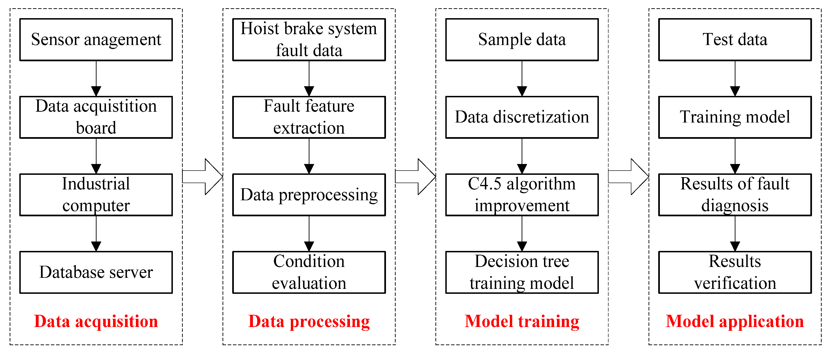
According to the needs of the fault diagnosis of the hoist brake system, this study established the general fault diagnosis frame of a mine hoist brake system based on machine learning, which is shown in Figure 2.

(1)

Data acquisition: The source of the data is mainly obtained from the monitoring system’s tracking of the operating state of the hoist brake system and the historical diagnostic knowledge base of the brake system. These data are characterized by large quantities, large numbers of dimensions, and rich content, which make up massive and heterogeneous large data. The collected data is stored in the SQL Server database. Also, the filtering and sorting function of the database can meet the low-cost storage requirements of massive and diverse data. Moreover, the data suitable for analysis can be filtered and integrated.

(2)

Data processing: Process the collected hoist brake system fault data, extract the fault features, denoise the data, process the missing values and continuous values of the sample data, and implement the K-means clustering algorithm by SPSS software. Finally, discretize continuous values.

(3)

Model training: Use the decision tree algorithm C4.5 to classify the sample data, add the Kendall concordance coefficient to improve the algorithm and use the improved C4.5 decision tree algorithm to train the sample data. Therefore, the decision tree classification model is obtained.

(4)

Model application: The data is trained to obtain the algorithm model, which generates fault diagnosis rules and judges the state of the brake system by classifying the data. These data are then applied to the fault diagnosis of the hoist brake system.

3. Data Acquisition and Pretreatment

3.1. Data Acquisition

The brake system of hoists includes disc brakes and hydraulic stations. The hoist brake system used in the laboratory has one brake disc on both sides of the drum, and also includes eight brake shoes and two hydraulic pipes. In the laboratory, by using displacement sensors, temperature sensors, pressure sensors, etc., to monitor or calculate the key parameters of the brake system directly or indirectly, the corresponding data is obtained. The specific monitoring parameters are shown in

Table 1. Brake system monitoring parameters.

No	Monitoring Attributes	Unit
X1-X2	Brake disc swing offset 1—Brake disc swing offset 2	mm
X3-X10	Brake shoe clearance 1—Brake shoe clearance8	mm
X11-X18	Brake force 1—Brake force 8	N
X19-X27	Brake shoe temperature 1—Brake shoe temperature 8	°C
X28	Hydraulic station oil pressure	MPa
X29	Pine gate oil pressure	MPa
X30	Hydraulic brake pressure	MPa
X31	Hydraulic station residual pressure	MPa
X32	Hydraulic station oil temperature	°C
X33	Lifting velocity	m/s
X34	Hoisting acceleration	m/s2
X35	Percentage of contact area between brake disc and brake shoe	%
…	…	…

.

After collecting the monitoring data, the SPSS data pretreatment method in the next subsection is used to analyze and process the fault eigenvalues, which can reduce the data dimension and reduce the computational workload.

3.2. SPSS-Based Data Pretreatment

SPSS is one of the current mainstream data analysis pieces of software, which can analyze the hoist operating state information contained in the data quickly. This analysis method can be applied to the processing and analysis of large amounts of data, providing a reliable scientific basis for analysts to make relevant decisions [19]. In the monitoring data’s pretreatment of the brake system, the relationship between the monitoring attributes is analyzed by SPSS, which has a certain enlightenment for the selection of the characteristic attributes in the decision tree. The following are the main treatment methods:

(1) Parameter test and interval estimation of data sets

In the trend’s estimation under the same working conditions, the estimation method of the confidence interval is usually adopted. In fact, the main body effect test and the estimation of the confidence interval can be realized conveniently in the SPSS. For example, by checking the main body effect between brake shoe clearance and the lifting velocity, hydraulic station oil temperature, and hydraulic station hydraulic pressure, it can be concluded that the brake shoe clearance has a significant influence on the lifting speed. As shown in

Table 2. Inter-subjective effect test results.

Source	Dependent Variable	Significant
Correction model	Hydraulic station oil temperature	0.059
	Hydraulic station oil pressure	0.073
	Lifting velocity	0.697
Intercept	Hydraulic station oil temperature	0.000
	Hydraulic station oil pressure	0.000
	Lifting velocity	0.000
Brake shoe clearance	Hydraulic station oil temperature	0.059
	Hydraulic station oil pressure	0.073
	Lifting velocity	0.697

.

(2) Correlation analysis and regression analysis

In data analysis, the correlation between parameters is usually analyzed, which mainly refers to the attribute relationship. For instance, models can be established under specific conditions or statistically compensated for missing values when dealing with missing values or prediction of fault. Faced with multi-attribute datasets in fault data, correlation analysis can establish correlations between attributes and make scientific estimates of future trends of data. Regression analysis mainly aims to predict the trend of future variables by optimizing the data over time and establish a functional relationship between variables. According to the analysis in SPSS, the lifting velocity and the acceleration have a linear correlation that can be used for dimensionality reduction. However, there is no correlation between the values of the brake shoe gaps. Therefore, this study only analyzes the fault of a single brake shoe by collecting data during the test.

(3) Cluster analysis

The cluster analysis mainly classifies the variables with high similarity to one class by calculating the affinity relationship between variables and displays the classification results in different ways. Since SPSS has an automatically generated cluster analysis model, the system itself can standardize the data, which solves the problem of normalizing and standardizing data. Cluster analysis can at the same time achieve data discretization. In this study, SPSS software is used to discretize the K-means clustering [20] of data continuity attributes, which is seen in Section 5.2 with the fault diagnosis experiment.

4. Decision Tree Classification Method

The commonly used decision tree classification algorithms are the ID3 and C4.5 algorithms. The ID3 algorithm uses the information gain criterion when selecting feature attributes and constructs the decision tree layer by layer. C4.5 is improved based on ID3. Besides the function of ID3 algorithm, C4.5 has the following advantages [21]: (1) using information gain rate as the basis for dividing attributes, the classification is more reasonable in the face of a few sample subsets; (2) it can process training samples containing both discrete and continuous data and training samples with attribute missing values; (3) multiple pruning methods are used to avoid redundant rules; (4) rules are easier to interpret and more accurate. Therefore, this study focuses on the in-depth analysis of the C4.5 algorithm.

The core idea of C4.5 is to set the training dataset $T$. When constructing the decision tree with dataset $T$, the attribute with the largest information gain rate is selected as the dividing node, and the data set $T$ is divided into $n$ subsets according to the current attribute partitioning standard. If one subset $T_i$ contains the same element class, the node is used as the leaf node and the partition is stopped. If the subset still contains different elements, it continues to divide according to the above division method recursively until all the elements of the subset belong to the same category. At last, nodes are no longer divided and are generated into trees instantly [22,23,24]. The specific process is:

Let $D$ be the training dataset and $\left|D\right|$ denote the size of the sample. Set $K$ to be a natural number, for all $k=1,2,\cdots ,K$, $C_k$ is a class. Assume that $\left|C_k\right|$ is the number of samples which belong to the class $C_k$ and ${\displaystyle \sum _{k=1}^K\left|C_k\right|}=\left|D\right|$. Suppose characteristic $A$ has different values $\{a_1,a_2,\dots ,a_n\}$. According to the value of the characteristic $A$, $D$ can be divided into $n$ subsets $D_1,D_2,\cdots ,D_n$, where, for each $i=1,2,\cdots ,n$, $\left|D_i\right|$ is the sample size of $D_i$, and ${\displaystyle \sum _{i=1}^n\left|D_i\right|}=\left|D\right|$. Denote the set of samples belonging to class $C_k$ in subset $D_i$ as $D_{ik}$, namely $D_{ik}=D_i\cap C_k$. Here, $\left|D_{ik}\right|$ is the sample size of $D_{ik}$.

Step 1: Calculate the empirical entropy $H\left(D\right)$

$$H\left(D\right)=-{\displaystyle \sum _{k=1}^K\frac{\left|C_k\right|}{\left|D\right|}}{\log }_2\frac{\left|C_k\right|}{\left|D\right|},$$

(1)

Step 2: Calculate the empirical conditional entropy $H\left(D|A\right)$

$$H\left(D|A\right)={\displaystyle \sum _{i=1}^n\frac{\left|D_i\right|}{\left|D\right|}}H\left(D_i\right)=-{\displaystyle \sum _{i=1}^n\frac{\left|D_i\right|}{\left|D\right|}}{\displaystyle \sum _{k=1}^K\frac{\left|D_{ik}\right|}{\left|D_i\right|}}{\log }_2\frac{\left|D_{ik}\right|}{\left|D_i\right|},$$

(2)

Step 3: Calculate the information gain

$$g\left(D,A\right)=H\left(D\right)-H\left(D|A\right),$$

(3)

Step 4: Calculate the information gain rate

$$g_R\left(D,A\right)=\frac{g\left(D,A\right)}{H_A\left(D\right)},$$

(4)

where

$$H_A\left(D\right)=-{\displaystyle \sum _{i=1}^n\frac{\left|D_i\right|}{\left|D\right|}}{\log }_2\frac{\left|D_i\right|}{\left|D\right|},$$

(5)

and $n$ is the number of characteristic $A$ values.

5. C4.5 Algorithm Improvement

The structure of the hoist brake system is complex and the cause of the failure is often not single, so the various failure factors should be taken into consideration. It is also worth noting that the relationship between the failure factors often has a significant impact on the fault. Therefore, in this study, when the decision tree goes to the step of selecting the optimal partition attribute, considering the correlation between attributes, Kendall concordance coefficient is introduced to improve C4.5 algorithm. Moreover, more accurate classification rules can be obtained based on keeping the advantages of the C4.5 algorithm.

5.1. Kendall Concordance Coefficient

The Kendall concordance coefficient can be used to calculate the degree of correlation between multiple levels of variables. Let $T$ represent the data set, consisting of $N$ attribute variables $X$ and $K$ decision variables $Y$. Set $B_k\left(k=1,2,\dots ,N\right)$ as the value of attribute $X$ and $R_i\left(i=1,2,\dots K\right)$ as the sum of each row of $B_k$. Here, $W$ denotes the Kendall concordance coefficient.

If the values in each attribute variable are different, the calculation formula is:

$$W=\frac{{\displaystyle \sum _{i=1}^K{R}_i^2}-\frac{{\left({\displaystyle \sum _{i=1}^K{R}_i}\right)}^2}{N}}{\frac{1}{12}{K}^2\left(N^3-N\right)},$$

(6)

If there are $m$ groups with the same value in each attribute variable, and the number of the same value is $m$, the calculation formula is:

$$W=\frac{{\displaystyle \sum _{i=1}^K{R}_i^2}-\frac{{\left({\displaystyle \sum _{i=1}^K{R}_i}\right)}^2}{N}}{\frac{1}{12}{K}^2\left(N^3-N\right)-K{\displaystyle \sum _{i=1}^N{T}_i}},$$

(7)

where

$$T_i={\displaystyle \sum _{i=1}^m\frac{n_i^3-n_i}{12}},$$

(8)

The Kendall concordance coefficient $W$ has a value between −1 and 1. If $W=-1$, then there is an opposite correlation between the variables. Also, if $W=1$, then there is a consistent correlation between the variables. On the other hand, if $W=0$, then there is no correlation between variables, namely, they are independent of each other.

5.2. Algorithm Optimization

Introduce the Kendall concordance coefficient $W$ into the C4.5 algorithm and simplify the formula. The process is:

Step 1: Calculate the correlation coefficient $W$ using formula (6) or (7).

Step 2: Introduce the coefficient $W$ into the formula (3) as follows:

$$g\left(D,A\right)=H\left(D\right)-H\left(D|A\right)\times W,$$

(9)

Step 3: According the base-change formula ${\log }_2^x=\frac{\ln x}{\ln 2}$ and the equivalent infinitesimal principle $\ln \left(1+x\right)\approx x$, the results obtained by simplifying formulas (1), (2), (4), and (5) are as shown in formulas (10)–(13).

$$\begin{array}{ll}H\left(D\right)& =-{\displaystyle \sum _{i=1}^K\frac{\left|C_k\right|}{N}}{\log }_2\frac{\left|C_k\right|}{N}=-{\displaystyle \sum _{i=1}^K\frac{\left|C_k\right|}{N}}\frac{\ln \frac{\left|C_k\right|}{N}}{\ln 2}\\ & =\frac{1}{N\ln 2}{\displaystyle \sum _{i=1}^K\frac{\left|C_k\right|\times \left(N-\left|C_k\right|\right)}{N}}\end{array}$$

(10)

$$\begin{array}{ll}H\left(D|A\right)& =-{\displaystyle \sum _{i=1}^n\frac{N_i}{N}}\times H\left(D_{ik}\right)={\displaystyle \sum _{i=1}^n\frac{N_i}{N}}\times \left(-{\displaystyle \sum _{i=1}^n\frac{N_{ik}}{N_i}\times \frac{\ln \frac{D_{ik}}{N_i}}{\ln 2}}\right)\\ & =\frac{1}{N\ln 2}{\displaystyle \sum _{i=1}^n{\displaystyle \sum _{k=1}^k\frac{D_{ik}\times \left(N_i-D_{ik}\right)}{N_i}}}\end{array}$$

(11)

$$\begin{array}{ll}{g}_R\left(D,A\right)& =\frac{g\left(D,A\right)}{H_A\left(D\right)}=\frac{H\left(D\right)-H\left(D|A\right)\times W}{H_A\left(D\right)}\\ & =\frac{{\displaystyle \sum _{k=1}^k\frac{C_k\times \left(N-C_k\right)}{N}-W\times {\displaystyle \sum _{i=1}^n{\displaystyle \sum _{k=1}^k\frac{D_{ik}\times \left(N_i-D_{ik}\right)}{N_i}}}}}{{\displaystyle \sum _{i=1}^n\frac{N_i\times \left(N-N_i\right)}{N}}}\end{array}$$

(12)

where

$$\begin{array}{cc}{H}_A\left(D\right)& =-{\displaystyle \sum _{i=1}^n\frac{N_i}{N}}{\log }_2\frac{N_i}{N}=-{\displaystyle \sum _{i=1}^n\frac{N_i}{N}}\times \frac{\ln \frac{N_i}{N}}{\ln 2}\\ & =\frac{1}{N\ln 2}{\displaystyle \sum _{i=1}^n\frac{N_i\times \left(N-N_i\right)}{N}}\end{array}$$

(13)

This study describes the improved C4.5 algorithm as K_C4.5.

5.3. Algorithm Implementation

The actual calculation process described below provides details about the implementation process of K_C4.5 algorithm optimization.

Table 3. Sample data set.

No	Condition Attribute				Decision Attribute
	A	B	C	D	F
1	3	2	2	1	1
2	1	1	1	3	1
3	2	3	2	1	0
4	2	1	2	2	0
5	1	2	1	2	1
6	3	2	2	3	0
7	3	3	2	1	1
8	1	2	2	1	0
9	2	2	1	1	0
10	3	3	2	2	0

is the sample data set.

As can be seen from Table 3, there are three attribute values in the condition attributes A, B, and D: 1, 2, 3, and C have two attribute values: 1, 2. There are two attribute values in the decision attribute F: 0,1. According to the attribute values in the table, the coefficient $W$ is first calculated, then the gain rate of each attribute is calculated with respect to the formula (12). After that, the decision tree is constructed according to the gain rate. The detailed steps are as follows:

First, each attribute is evaluated according to the rating method. Assuming that the grade of 0 in the decision attribute F is higher than 1, then the probabilities that the three attribute values in A are obtained as: $P\left(A_1\right)=\frac{1}{6}$, $P\left(A_2\right)=\frac{1}{2}$, and $P\left(A_3\right)=\frac{1}{3}$. Obviously, $P\left(A_2\right)>P\left(A_3\right)>P\left(A_1\right)$. Similarly, we can get $P\left(B_2\right)>P\left(B_3\right)>P\left(B_1\right)$ in attribute B, $P\left(C_2\right)>P\left(C_1\right)$ in attribute C, and $P\left(D_1\right)>P\left(D_2\right)>P\left(D_3\right)$ in attribute D. The results of grade evaluation are shown in

Table 4. Grade evaluation results.

No	Condition Attribute				Decision Attribute
	A	B	C	D	F
1	5.5	3	4	3	8.5
2	9	9.5	9	9.5	8.5
3	2	7	4	3	3.5
4	2	9.5	4	7	3.5
5	9	3	9	7	8.5
6	5.5	3	4	9.5	3.5
7	5.5	7	4	3	8.5
8	9	3	4	3	3.5
9	2	3	9	3	3.5
10	5.5	7	4	7	3.5

.

Then, Calculate the coefficient $W$ by using Equations (6) and (7) according to the data in Table 4.

Calculate the sum of the first line of conditional attribute values as:

$$R_1=5.5+3.0+4.0+3.0=15.5$$

Similarly, the values of the other rows are $R_2=37$, $R_3=16$, $R_4=22.5$, $R_5=28$, $R_6=22$, $R_7=19.5$, $R_8=19$, $R_9=17$, $R_{10}=23.5$.

According to formula (8):

$$T_1={\displaystyle \sum _{i=1}^m\frac{n_i^3}{12}}=\frac{3^3-3}{12}+\frac{3^3-3}{12}+\frac{4^3-4}{12}=9$$

In the same way, $T_2=12.5$, $T_3=30$, $T_4=12.5$. Thus,

$$W=\frac{{\displaystyle \sum _{i=1}^K{R}_i^2}-\frac{{\left({\displaystyle \sum _{i=1}^K{R}_i}\right)}^2}{N}}{\frac{1}{12}{K}^2\left(N^3-N\right)-K{\displaystyle \sum _{i=1}^N{T}_i}}=\frac{\left({15.5}^2+{37}^2+\dots +{23.5}^2\right)-\frac{{\left(15.5+37+\dots +23.5\right)}^2}{10}}{\frac{1}{12}\times 4^2\times \left({10}^3-10\right)-4\times \left(9+12.5+30+12.5\right)}=0.359$$

The information gain of each attribute is calculated by formula (10):

$${\displaystyle \sum _{k=1}^K\frac{C_k\times \left(N-C_k\right)}{N}}=\frac{6\times \left(10-6\right)}{10}+\frac{4\times \left(10-4\right)}{10}=4.8$$

$$\begin{array}{l}W\times {\displaystyle \sum _{i=1}^n{\displaystyle \sum _{k=1}^K\frac{C_k\times \left(N_i-C_k\right)}{N_i}}}\\ =0.359\times \left(\frac{1\times \left(3-1\right)}{3}+\frac{2\times \left(3-2\right)}{3}+\frac{2\times \left(4-2\right)}{4}+\frac{2\times \left(4-2\right)}{4}\right)\\ =1.197\end{array}$$

$$\begin{array}{l}{\displaystyle \sum _{i=1}^n\frac{N_i\times \left(N-N_i\right)}{N}}=\frac{3\times \left(10-3\right)}{10}+\frac{3\times \left(10-3\right)}{10}+\frac{4\times \left(10-4\right)}{10}\\ =6.6\end{array}$$

$$Gain\left(A\right)=\frac{4.8-1.197}{6.6}=0.546$$

Analogously, the gain rates of several other attributes are given as $Gain\left(B\right)=0.5$, $Gain\left(C\right)=0.785$, and $Gain\left(D\right)=0.5$. Since $Gain\left(C\right)>Gain\left(A\right)>Gain\left(B\right)=Gain\left(D\right)$, condition attribute C should be selected as the root attribute.

6. Experimental Verification

In this study, the 2JTP-1.2 hoist in laboratory is used as the test object to test and verify the diagnostic model generated by the algorithm. The fault data is collected through simulation test faults, then the diagnostic rules are used for fault diagnosis and prediction. The improved algorithm is then compared to the original. In this study, the algorithm is implemented in Python language [25,26].

6.1. Fault Simulation

Since the fault cannot be specifically set in actual production, it is necessary to put up a test rig in the laboratory to perform a fault simulation test. The monitoring data is collected in the fault state. In this test, the parameters of the brake system are adjusted to simulate the faults and mixed faults of each brake system. Also, the correctness of diagnosis is verified. These parameters include brake disc swing offset, brake shoe clearance, and hydraulic station residual pressure. The specific fault simulation method is as follows [27]:

(1) Change brake shoe clearance test

Step 1: Start the hydraulic pump and turn the switch to the rope adjustment indicator so that the hand brake in the released state. At this moment, the brake oil pressure of the brake system is 4.8 Mpa;

Step 2: Take out the hexagon socket head bolts in the center of the brake disc and loosen the larger bolts in the center of the brake disc. Carry out the same operation on other brake discs, and keep the number of turns of the bolt on the same side to loosen the consistent bolt;

Step 3: Turn the switch to the normal indication and run the hoist, then collect the data.

(2) Change brake disc swing offset test

Step 1: Start the hydraulic pump when the hoist is stopped. After this, turn the switch to the rope adjustment indicator to ensure that the hand brake is in the fully released state. Thereafter, turn off the hand brake switch of one side of the oil way. At this time, the oil circuit brake is in the fully released state and does not participate in the brake work of the hoist;

Step 2: Adjust the brake shoe clearance of the oil circuit brake on the other side;

Step 3: Turn the switch to the normal indication and run the elevator. Then, brake and repeat the brake operation. After this process, collect the data.

(3) Chang hydraulic station residual pressure

Step 1: Start the hydraulic pump in the state of parking and turn the switch to the indication of the rope adjustment so that the hand brake is in a tight state. The oil pressure at this stage is 0.2 MPa;

Step 2: Adjust the screw on the far-right side of the oil pressure gauge to make the residual pressure of the system reach 0.3–1 MPa. Finally, collect the data to observe the brake effect.

Combined with the test conditions, the fault types simulated by adjusting the above parameters include: brake shoe clearance is too small, brake disc overheating, idle motion time is too long, emergency brake fault, residual pressure is too large, disc spring fault and normal, etc. The fault types are numbered as shown in

Table 5. Fault types.

No	Fault Types
F1	Brake shoe clearance is too small
F2	Brake disc overheating
F3	Idle motion time is too long
F4	Emergency brake fault
F5	Residual pressure is too large
F6	Disc spring fault
F7	Normal

.

6.2. Fault Diagnosis

The data used in the test includes not only normal operating data but also various brake system fault data, and the data set used to train the model is extracted from the historical database monitored by the hoist brake system. The decision tree algorithm constructs the model by mining the hidden fault law from the historical monitoring data of the hoist brake system and extracting the diagnostic rules that can provide the basis for the hoist fault diagnosis.

The redundant data is removed by the above-mentioned SPSS analysis and pretreatment of the data and the relevant feature data is retained for the diagnosis of the above-mentioned fault. Fault analysis test data mainly includes X1-brake shoe clearance, X2-hydraulic station residual pressure, X3-the contact area between disc and brake shoe, X4-brake disc swing offset, and other characteristic attributes. Simulate every fault and collect test data. Some data are displayed in the

Table 6. Partial fault data set.

Condition Attributes				Decision Attribute
X1	X2	X3	X4	F
0.86	0.43	85	0.34	F1
2.26	0.48	55	0.15	F2
0.79	0.37	86	0.27	F1
1.35	0.54	85	0.31	F5
2.36	0.35	89	0.25	F3
1.37	0.42	76	0.85	F6
1.28	0.21	91	0.37	F4
2.25	0.47	57	0.16	F2
…	…	…	…	…

. Take K = 4 (number of conditional attributes), use SPSS to perform K-means clustering discretization processing. The results will be displayed in

Table 7. Data discretization.

Condition Attributes				Decision Attribute
X1	X2	X3	X4	F
2	1	2	1	F1
3	1	1	1	F2
2	1	2	1	F1
1	3	2	1	F5
3	1	2	1	F3
1	1	2	2	F6
1	2	2	1	F4
3	1	1	1	F2
…	…	…	…	…

.

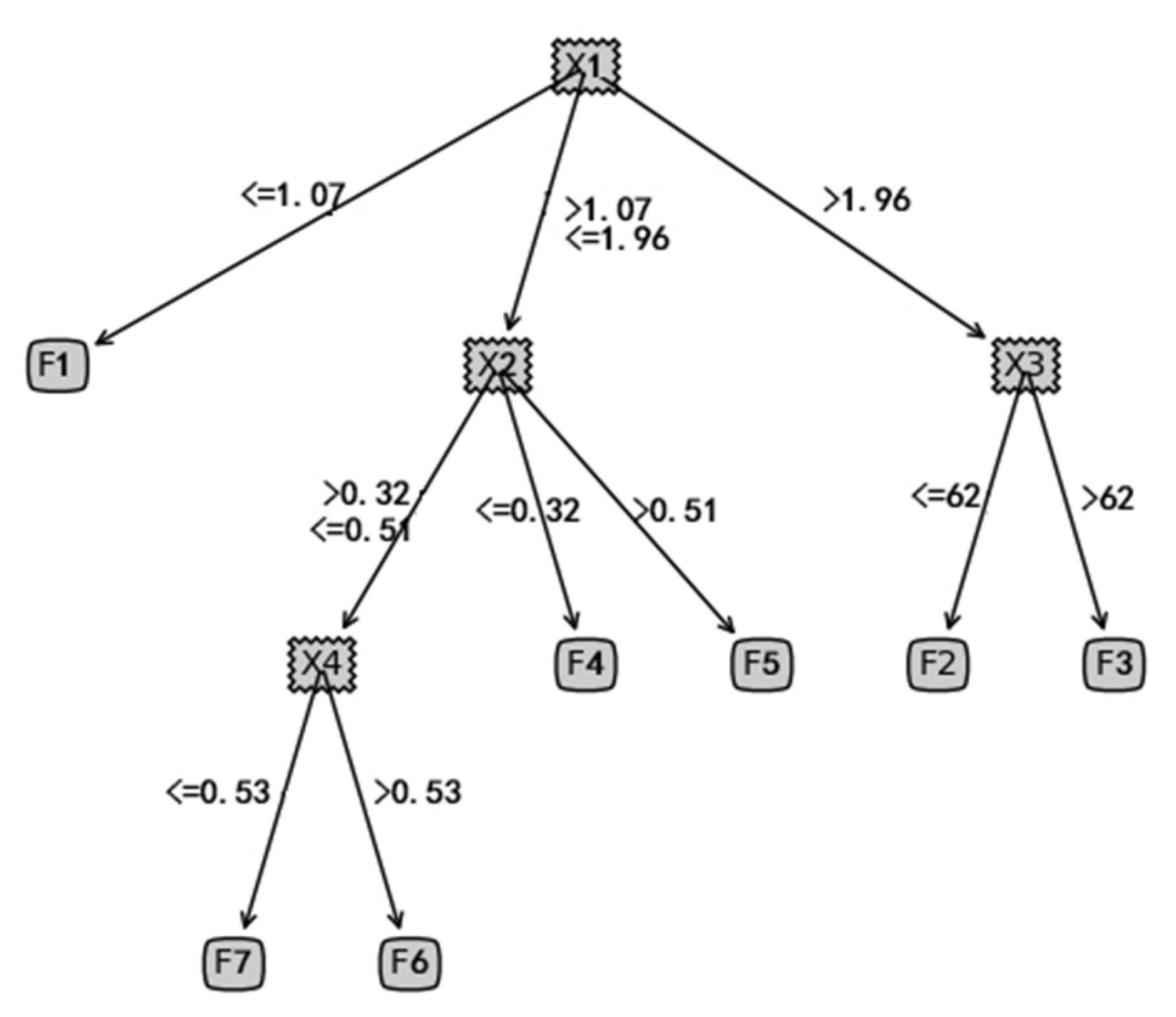
After importing the Table 7 data set into the K_C4.5 algorithm, the decision tree is generated via Python. The results are shown in Figure 3.

After using the Python program to get the classification model of the K_C4.5 decision tree, generate diagnostic rules.

Table 8. The fault data set generates rules under the K_C4.5 algorithm.

No	Rules
1	If brake shoe clearance <=1.07 then F1 occurrence
2	If brake shoe clearance >1.96 and contact area <=62% then F2 occurrence
3	If brake shoe clearance >1.96 and contact area >62% then F3 occurrence
4	If 1.07< brake shoe clearance <=1.96 and hydraulic station residual pressure <=0.32 then F4 occurrence
5	If 1.07< brake shoe clearance <=1.96 and hydraulic station residual pressure >0.51 then F5 occurrence
6	If 1.07< brake shoe clearance <=1.96 and 0.32< hydraulic station residual pressure <=0.51 and brake disc swing offset >0.53 then F6 occurrence
7	If 1.07< brake shoe clearance <=1.96 and 0.32< hydraulic station residual pressure <=0.51 and brake disc swing offset <=0.53 then F7 occurrence

shows the results.

6.3. Result Analysis

(1) Classification accuracy test

The authors collected 100 sets of data of various fault data to test the above diagnostic rules. The results of the tests appear in

Table 9. Diagnostic rule test results.

Fault Type	Number of Test Samples	Number of Correctly Classified Samples	Accuracy
Brake shoe clearance is small	100	97	97%
Brake disk overheating	100	98	98%
Cavity time is too long	100	92	92%
Emergency brake fault	100	96	96%
Residual pressure is too large	100	94	94%
Disc spring fault	100	99	99%
Normal	100	100	100%

. The classification accuracy is up to 95.85%, and the model meets the classification accuracy requirements.

(2) Evaluation index analysis before and after algorithm improvement

This study uses the following evaluation indicators to test the performance of the algorithm before and after improvement: decision tree size, number of decision rules, tree building time, correct classification percentage, and difference degree (Kappa statistic). Among them, the decision tree size refers to the total number of nodes generated, the number of decision rules refers to the number of diagnosis rules finally generated, and the Kappa statistic $K$ is used to evaluate the difference between the classification result of the classifier and the random classification. $K=1$ indicates that the classifier is completely different from the random classification. $K=0$ indicates that the classifier is the same as the random classification and has no classification effect. The closer the value is to 1, the better. The results of the tests appear in

Table 10. Analysis of evaluation in different algorithms using fault samples.

Evaluation Index	C4.5	K_C4.5
Decision tree size	17	11
Number of decision rules	9	7
Tree building time (s)	0.06	0.02
Correct classification Percentage (%)	85.4	95.85
Difference degree	0.9278	0.9571

.

(3) Accuracy test before and after algorithm improvement in big data samples

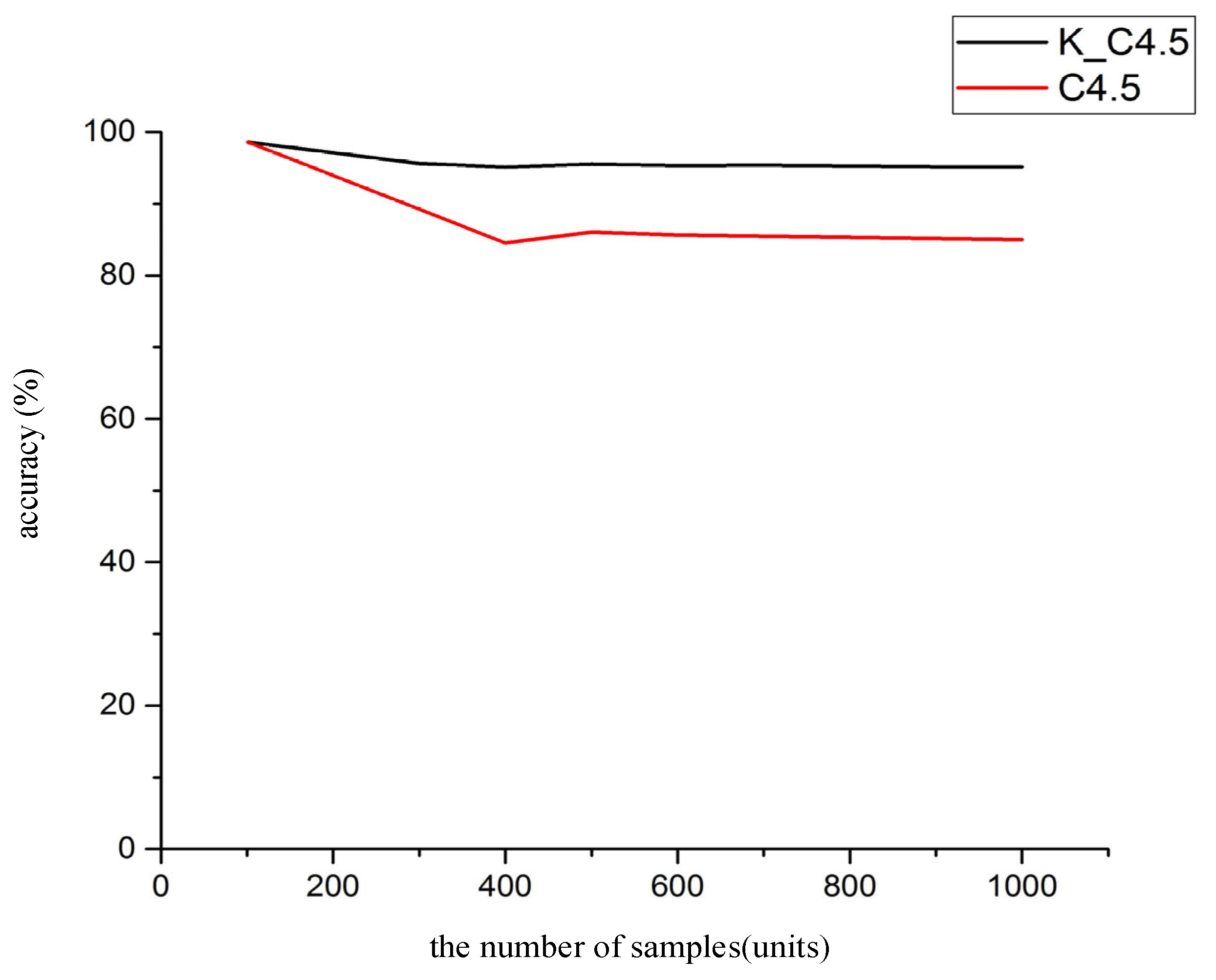
To better test the accuracy change of the C4.5 algorithm before and after improvement, this study observes the change of accuracy by increasing the number of samples (taking 1000 samples). The samples are classified according to the diagnostic rules generated by K_C4.5 algorithm and the original C4.5 algorithm. The accuracy of the final test results is shown in Figure 4.

Figure 4 shows that the accuracy of the two algorithms is similar when the number of samples is small, but with the increase of the number of samples, it can be seen that the accuracy of K_C4.5 algorithm is significantly higher than the original C4.5 algorithm, and gradually stabilizes at a higher level.

7. Conclusions

(1)

A fault diagnosis method of mine hoist brake systems based on machine learning is proposed, and the corresponding fault diagnosis model is established. This method is based on data and can meet the needs of fault diagnosis in a big data environment.

(2)

A dynamic decision-making model based on C4.5 decision tree is established. The model takes information gain rate as the basis of attribute partition and can deal with training sets with small sample subsets, and discrete and continuous data. It can also deal with training samples with missing attributes. In addition to these, the model considers the correlation between attributes and introduces Kendall concordance coefficient to the process of establishing a decision tree. More accurate classification rules can be obtained.

(3)

Through the fault simulation and comparison test, the validity and diagnostic accuracy of the diagnostic method are verified. The improved C4.5 decision tree classification algorithm can effectively improve the diagnostic efficiency and reliability.

(4)

This study focuses on the application of decision tree algorithm in the fault diagnosis of hoist brake system, and the specific application of other machine learning algorithms in fault diagnosis can be further studied, especially the improvement of the algorithm needs to be further explored to make it more in line with the data characteristics of the hoist, which will become the focus of the author’s next research.

References

1. Xu, G.; Song, D.; Zhang, D.; Zhang, X.; Sha, S. A novel mechanical design of disc brakes for fault diagnosis and monitoring positive braking pressure in mine hoist. Adv. Mech. Eng. 2019, 11, 1687814019842494. [Google Scholar] [CrossRef] [Green Version]
2. Giraud, L.; Galy, B. Fault tree analysis and risk mitigation strategies for mine hoists. Saf. Sci. 2018, 110, 222–234. [Google Scholar] [CrossRef]
3. Li, J.J.; Hu, L.M.; Meng, G.Y. Fault Diagnosis for Constant Deceleration Braking System of Mine Hoist Based on Principal Component Analysis and SVM. In Proceedings of the International Conference on Electronic Information Technology and Computer Engineering, Zhuhai, China, 23–24 September 2017. [Google Scholar]
4. Lei, Y.T. Study on SOM Neural Network Applied to the Fault Diagnosis of Hoist Brake System. In Proceedings of the International Conference on Control Engineering and Automation, Chongqing, China, 29–30 November 2014. [Google Scholar]
5. Li, J.L.; Yang, Z.J.; Pang, X.Y. Intelligent fault diagnosis methods of mine hoist based on knowledge engineering. J. China Coal Soc. 2016, 46, 1309–1315. [Google Scholar]
6. Li, J.L.; Wang, J.; Yang, Z.J. Fault diagnosis of mine hoist braking system based on three layers information fusion. J. Vib. Meas. Diagn. 2018, 38, 1–6. [Google Scholar]
7. Li, J.; Xie, J.; Yang, Z.; Li, J. Fault diagnosis method for a mine hoist in the internet of things environment. Sensors 2018, 18, 1920. [Google Scholar] [CrossRef] [Green Version]
8. Li, J.; Liu, Y.; Xie, J.; Li, M.; Sun, M.; Liu, Z.; Jiang, S. A remote monitoring and diagnosis method based on four-layer IoT frame perception. IEEE Access 2019, 7, 144324–144338. [Google Scholar] [CrossRef]
9. Askarian, M.; Escudero, G.; Graells, M.; Zarghami, R.; Jalali-Farahani, F.; Mostoufi, N. Fault diagnosis of chemical processes with incomplete observations: A comparative study. Comput. Chem. Eng. 2016, 84, 104–116. [Google Scholar] [CrossRef] [Green Version]
10. Liu, T.; Zhao, H.M. Early warning system design of mine hoist fault based on decision tree. Comput. Simul. 2012, 29, 228–513. [Google Scholar]
11. Li, J.L.; Yang, Z.J. An uncertain reasoning method of hoist fault diagnosis. J. China Coal Soc. 2014, 39, 586–592. [Google Scholar]
12. Vernekar, K.; Kumar, H.; Gangadharan, K.V. Fault diagnosis of deep groove ball bearing through discrete wavelet features using support vector machine. Int. J. Comadem 2014, 17, 31–37. [Google Scholar]
13. Yao, D.; Yang, J.; Cheng, X.; Wang, X. Railway rolling bearing fault diagnosis based on muti-scale IMF permutation entropy and SA-SVM classifier. J. Mech. Eng. 2018, 54, 168–176. [Google Scholar] [CrossRef]
14. He, Q.; Li, N.; Luo, W.J.; Shi, Z.Z. A survey of machine learning algorithms for big data. Pattern Recognit. Artif. Intell. 2014, 27, 327–336. [Google Scholar]
15. Ibrahim, M.; Parrish, D.J.; Brown, T.W.C.; McDonald, P.J. Decision tree pattern recognition model for radio frequency interference suppression in NOR experiments. Sensors 2019, 19, 3153. [Google Scholar] [CrossRef] [PubMed] [Green Version]
16. Kang, M.; Srivastava, P.; Adve, V.; Kim, N.S.; Shanbhag, N.R. An energy-efficient programmable mixed-signal accelerator for machine learning algorithms. IEEE Access 2019, 39, 64–72. [Google Scholar] [CrossRef]
17. Kwon, H.Y.; Kim, N.J.; Lee, C.K.; Won, C. Searching magnetic states using an unsupervised machine learning algorithm with the Heisenberg model. Phys. Rev. B 2019, 99, 024423. [Google Scholar] [CrossRef]
18. Shao, H.; Wang, L.W.; Ji, Y.F. Link prediction algorithms for social networks based on machine learning and HARP. IEEE Access 2019, 7, 122722–122729. [Google Scholar] [CrossRef]
19. Vanus, J.; Kubicek, J.; Gorjani, O.M. Using the IBM SPSS SW tool with wavelet transformation for CO2 Prediction within IoT in smart home care. Sensors 2019, 19, 1407. [Google Scholar] [CrossRef] [Green Version]
20. Han, Q.Q.; Liu, J.M.; Shen, Z.W. Vector partitioning quantization utilizing K-means clustering for physical layer secret key generation. Inf. Sci. 2020, 512, 137–160. [Google Scholar] [CrossRef]
21. Gupta, J.; Patrick, J.; Poon, S. Clinical Safety Incident Taxonomy Performance on C4.5 Decision Tree and Random Forest. Stud. Health Technol. Inform. 2019, 26, 83–88. [Google Scholar]
22. Yang, Y.; Chen, W.G. Taiga: Performance optimization of the C4.5 decision tree construction algorithm. Tsinghua Sci. Technol. 2016, 21, 415–425. [Google Scholar] [CrossRef]
23. Han, L.; Li, W.H.; Su, Z. An assertive reasoning method for emergency response management based on knowledge elements C4.5 decision tree. Expert Syst. Appl. 2019, 122, 65–74. [Google Scholar] [CrossRef]
24. Mu, Y.; Liu, X.; Yang, Z.; Liu, X. A parallel C4.5 decision tree algorithm based on MapReduce. Concurr. Comput. Pract. Exp. 2017, 29, e4015. [Google Scholar] [CrossRef]
25. Kadiyala, A.; Kunar, A. Applications of python to evaluate environmental data science problems. Environ. Prog. Sustain. Energy 2017, 36, 1580–1586. [Google Scholar] [CrossRef]
26. Sarradj, E.; Herold, G. A Python framework for microphone array data processing. Appl. Acoust. 2017, 116, 50–58. [Google Scholar] [CrossRef]
27. Li, J.L.; Fan, Z. Fault diagnosis for braking system of mine hoist based on BN and A-Star. Min. Res. Dev. 2018, 38, 116–120. [Google Scholar]
Figure 1. Structure of mine hoist brake system.
Applsci 10 01768 g001
Figure 2. Fault diagnosis frame of mine hoist brake system based on machine learning.
Applsci 10 01768 g002
Figure 3. K_C4.5 decision tree classification result.
Applsci 10 01768 g003
Figure 4. Comparison of the accuracy of the two algorithms.
Applsci 10 01768 g004