Co-Processing Parallel Computation for Distributed Optical Fiber Vibration Sensing

Abstract

Rapid data processing is crucial for distributed optical fiber vibration sensing systems based on a phase-sensitive optical time domain reflectometer (Φ-OTDR) due to the huge amount of continuously refreshed sensing data. The vibration sensing principle is analyzed to study the data flow of Rayleigh backscattered light among the different processing units. A field-programmable gate array (FPGA) is first chosen to synchronously implement pulse modulation, data acquisition and transmission in parallel. Due to the parallelism characteristics of numerous independent algorithm kernels, graphics processing units (GPU) can be used to execute the same computation instruction by the allocation of multiple threads. As a conventional data processing method for the sensing system, a differential accumulation algorithm using co-processing parallel computation is verified with a time of 1.6 μs spent of the GPU, which is 21,250 times faster than a central processing unit (CPU) for a 2020 m length of optical fiber. Moreover, the cooperation processes of the CPU and GPU are realized for the spectrum analysis, which could shorten substantially the time of fast Fourier transform analysis processing. The combination of FPGA, CPU and GPU can largely enhance the capacity of data acquisition and processing, and improve the real-time performance of distributed optical fiber vibration sensing systems.

1. Introduction

A distributed optical fiber vibration sensing system has the advantages of a simple structure, resistance to electromagnetic interference, adaptability in flammable environments and wide detection range [1,2,3]. As one typical distributed optical fiber vibration sensing system, a phase-sensitive optical time domain reflectometer (Φ-OTDR) can achieve simultaneously multi-point vibration detection and location. Because of the benefits of its high sensitivity, good spatial resolution and long detecting distance [4,5], Φ-OTDR has broad application prospects in long-distance oil and gas pipelines [6], border security intrusion detection and smart grids [7,8]. The current research hotspot of Φ-OTDR is the improvement of its sensing performance, such as a sensing distance up to even hundreds of kilometers [9,10], and a spatial resolution of a sub-meter magnitude [11], which leads to a huge amount of sensing data and a growing demand for computation resources. Consequently, the time consumption procedure of signal processing is longer and the real-time performance is more degradative. In order to solve this issue, many researchers have studied computational enhancement technologies for distributed optical fiber vibration sensing.

The preprocessing of Rayleigh backwards scattering (RBS) curves incurs costs in the major computing resource of the central processing unit (CPU). Many studies about the algorithm improvement of preprocessing have been proposed. Traditional and classical data preprocessing methods, such as the moving average method, moving differential method [12,13] and frequency spectrum analysis have been widely used in a Φ-OTDR system [14,15]. In 2017, [16] proposed a novel single-source dual heterodyne detection scheme to improve the optical path of the system. It can reduce the data volume in order to shorten the response time and improve the real-time performance of the system. The authors of [17] used a data matrix matching algorithm to optimize the data demodulation process of the Φ-OTDR system. By reducing the total amount of data needed for sensing data demodulation, the system calculation time is reduced and the real-time performance of the system is improved. It must be noted that, in previous related work, the authors reduced the amount of data to shorten the overall running time of the system.

As these preprocessing methods are always performed by a single-thread computing system based on a CPU, the massive amount of data in the Φ-OTDR system could lead to a longer processing time and even result in a system crash. Thus, the concurrent computation technology based on a graphics processing unit (GPU) could be used for large-scale data parallel processing, which can effectively enhance the processing speed of massive data [18,19,20]. Hui et al. first demonstrated the method of applying a GPU, which is good at parallel computing, to a Φ-OTDR sensing system, in order to provide a frequency spectrum analysis of the system, while the real-time performance of the system was not studied [21]. Sha et al. also used GPU for dealing with the data of a Φ-OTDR sensing system, so the speed of data processing was enhanced and the real-time performance was optimized [22]. The studies on GPU-parallel computing also have been applied to other fields, such as Fiber Bragg Grating (FBG) sensor and Stimulated Brillouin scattering (SBS) in optical telecommunication systems [23,24]. The fields of cellular and remote sensor imaging [25] and the occupancy grid maps in automotive environments also utilized GPU-parallel technology to improve real-time performance [26].

However, the high-speed concurrent computation can hardly do without the support of high-speed data acquisition, particularly in the process of real-time collection of vibration information in time, space, and frequency.

In this paper, without changing the amount of data in the system, we reduce the overall running time of the system by optimizing data acquisition and data demodulation methods. A novel data co-processing parallel computation method is demonstrated, which combines the field programmable gate array (FPGA) technology with CPU and GPU processing. Specifically, the generation of an external modulation pulse signal and the acquisition of RBS light signals are realized simultaneously by using the FPGA technology with parallel operation characteristics in the hardware. The differential accumulation algorithm and fast Fourier transform (FFT) of RBS curves are realized by using the GPU technology alongside the parallel computing advantages of the software. The contrast diagram of the internal structures of the FPGA, CPU and GPU is shown in Figure 1. As illustrated in Figure 1a, FPGA technology is programmable and flexible, meaning it can can synchronously implement multiple tasks, such as pulse modulation, data acquisition and transmission [27,28]. In Figure 1b, the CPU has many complex control units and a lot of cache space. In Figure 1c, the GPU has a macroscopic parallel structure containing two graphics processing clusters (GPC). Each GPC includes a raster engine and multiple polymorph engines, texture processing clusters (TPC) and a stream processor (SM). Each SM has 128 arithmetic logical units (ALU) which are used to realize parallel computation. Therefore, the CPU is an expert in logical control and computing different types of data, while the GPU is suitable for large-scale data parallel computing [29,30,31]. In summary, the advantage of this combination is the improvement of the real-time performance of the sensing system, achieving the high-speed detection and location of the vibration signal in the practical long-distance application situations. However, it also has a lot of room for improvement. For example, the current common problem of internal signal communication overhead can be solved by optimizing the shared memory communication mechanism between execution units [32].

2. Φ-OTDR System Principle

2.1. Vibration Sensing Principle

The vibration sensing principle of the Φ-OTDR system is based on the phenomenon of Rayleigh backwards scattering (RBS) light, which is produced by the elasto-optical effect in the inner of optical fiber, when the pulsed light is injected into and propagates along the optical fiber. The result of the mutual interference of numerous Rayleigh scattering centers within the injected pulse duration lead to the formation of random up and down fluctuations in the RBS curve. When a light pulse with a frequency of w is injected into the sensing optical fiber at the moment of t = 0, the amplitude of backscattered signal without vibration is shown in the following equation [33]:

$$r\left(t\right)={\displaystyle \sum _{p=1}^{\mathrm{M}}{\mathrm{I}}_p}\times \exp \left[j\mathsf{\omega }\left(t-{\mathsf{\tau }}_p\right)\right]\times \exp \left(-\mathsf{\beta }\frac{c{\mathsf{\tau }}_p}{n_{}}\right)\times \mathrm{F}\left(\frac{t-{\mathsf{\tau }}_p}{\mathrm{L}}\right)$$

(1)

where I_p and τ_p are respectively the amplitude and the time delay of the p-th RBS curve; L means the pulse width of incident pulse; β is the fiber attenuation constant; c is the velocity of light in a vacuum; n is the refractive index of the fiber; M is the number of scatters within the sensing fiber. The F(t/L) is a rectangular function, which can be expressed as:

$$\mathrm{F}\left(\frac{t}{\mathrm{L}}\right)=\{\begin{array}{cc}1,& 0\le \frac{t}{L}\le 1\\ 0,& \frac{t}{L}\le 0,\frac{t}{L}\ge 1\end{array}$$

(2)

When an external vibration is applied at certain positions in the sensing optical fiber, the light phase will be modulated, which could be collected by the intensity detection. In general, the acquired data should be processed by a differential accumulation algorithm and an FFT algorithm in order to demodulate the vibration location and frequency information [34,35]. Eventually, the detection and location of external vibration could be achieved based on the RBS curves.

2.2. Experiment Setup

The experiment setup is illustrated in Figure 2 based on the principle of the Φ-OTDR sensing system. The laser source has an ultra-narrow linewidth of 100 Hz and a center wavelength of 1550 nm. The polarization state of the output laser will be affected by the birefringence property of the optical fiber. Therefore, the polarization controller is used to adjust the polarization state of the laser [36]. The FPGA module drives the acousto-optical modulator (AOM) to modulate the continuous light into pulsed light, while the repetition frequency is 8 kHz and the pulse width is 200 ns, which corresponds to 20 m spatial resolution. More concretely, the FPGA board generates a series of clock sequences with an adjustable repetition frequency and pulse width in the form of a transistor–transistor logic (TTL) signal, which is amplified by the boost circuit to adapt the input voltage of AOM. This electrical modulation signal acts on the electroacoustic transducer of AOM, then transforms into the ultrasonic field in the form of electrical signal. When the light wave passes through the acousto-optic medium, due to the acousto-optic effect, the continuous light is modulated and becomes the intensity modulation wave in the form of an optical pulse. Then, the pulse is injected into an erbium-doped fiber amplifier (EDFA), which could amplify the power of the pulsed light. Following this, the pulsed light goes through a dense wavelength division multiplexer (DWDM), which can combine and transmit different wavelengths in the same fiber. Therefore, the light, including other wavelengths (except 1550 nm), could be filtered out by the DWDM, and a purer optical wave at 1550 nm could be obtained at the output of the DWDM module. Then, the pulsed light is launched into the sensing optical fiber via an optical circulator (OC). A piezoelectric transducer (PZT) is placed on a certain location of the sensing optical fiber in order to produce a vibration signal. Eventually, the coherent RBS light is monitored by the photodetector (PD) and is then transformed into an electric signal. The FPGA board could realize the data acquisition with the hardware language of VerilogHDL and the parallel programming tool Quartus II. In the host computer, the type of CPU is a CORE i7 8700K, using C programming language and the Visual Studio programming tool.

2.3. Data Flow Analysis

As illustrated in Figure 3, the complete Φ-OTDR system consists of a data generation unit, a data acquisition unit and a data processing unit. Firstly, the modulated pulse which is launched into the Φ-OTDR sensing system continuously generates RBS curves, then the optical signal is detected by PD and converted to an electronic signal. Secondly, the electric signal is acquired by an analog–digital converter (ADC) with a 50 MSa/s sample rate, then stored in the on-chip RAM of FPGA. Owing to a large amount of RBS data collected by the Φ-OTDR sensing system, as well the insufficient internal storage space of the FPGA, this will result in data overflows and even the collapse of the whole system if the data is not sent to the host computer in time. Therefore, FPGA must complete the old data which are stored in the on-chip RAM, preprocessing and transmitting them into the CPU before the arrival of new data. The FPGA module is connected to the CPU via a USB transmission interface, achieving data transmission quickly. Eventually, when the amount of data reaches a certain level, the data can be transferred from the CPU to the GPU, in order to realize fast algorithmic processing. Afterwards, the GPU sends data back to the CPU after dealing with data through multi-threads, then the results can be displayed on the screen.

3. Data Parallel Processing Principle

3.1. Data Parallel Processing Based on FPGA

Owing to the large amount of RBS data collected by the Φ-OTDR sensing system and the demand for real-time data acquisition, the FPGA of Altera’s Cyclone III series is chosen to implement pulse modulation, data acquisition and data transmission in parallel. The main functions of the FPGA in the Φ-OTDR sensing system are shown in Figure 4.

Firstly, the AOM controller generates a pulse signal whose repetition frequency and width are 8 kHz and 200 ns, respectively, in the way of FPGA programming. Then, the pulse signal is transferred to the AOM in order to transform continuous light into the expected pulsed light via the Input/ Output (I/O) interface. Furthermore, the operation of the main module depends on the clock domain management which is realized by phase locked logic (PLL). It receives a reference clock generated from a crystal oscillator and provides clocks of 50 and 100 MHz for the A/D controller and the USB controller, respectively.

Secondly, the Syn module synchronously controls the A/D controller to enable the acquisition state and dominate sampling rate. The operating principle of the A/D controller is based on the state machine. State 0 is the initial state and turns into State 1 when the synchronous trigger signal arrives. State 1 runs in a continuous loop until the data counter is full, then it changes into State 2. The additional data header should be added to each RBS data string in State 2. State 3 means that the data is written into the internal memory.

Thirdly, a first-in first-out (FIFO) device is used as the memory module to temporarily store the collected data. The data are written to FIFO and read out to the upper computer at the speeds of 50 and 100 MB/s, respectively. This method is mainly used in order to achieve data storage and balance the speed of data writing and reading, in case useless data is transmitted.

Afterwards, the USB controller is used to control the data transmission between FIFO and the high-speed USB 3.0 transmission microcontroller (EZ-USB FX3). It is also a state machine which consists of three states. State 0 represents the start state, which changes into State 1 when the RBS data arrives from the FIFO. State 1 is the full flag judgment state. If the slave device, FIFO, that exits in EZ-USB FX3 is not full, it moves to State 2, otherwise, it remains in State 1. State 2 represents the data writing state. During this state, the RBS data can be read and then written into the slave FIFO through the synchronized slave FIFO device at a speed of 100 MB/s. Finally, the EZ-USB FX3 chip packages the received data and transmits the data to the host computer via the USB transmission bus.

In summary, the core functionality of the FPGA board is to generate a pulse similar to a trigger signal, then data acquisition, local storage and data transmission via the serial bus. These functions could further affect the parameters of The Φ-OTDR system. For example, the data acquisition speed is 50 MSa/s and the data transmission speed is 100 MB/s in our experimental setup, which means that the real-time data throughput should be approximately equal or less than 100 MB/s. On one hand, the data acquisition speed could determine the resolution in the distance. Supposing that the interval between the sending and receiving time of the sensing light is 1 s, the maximum propagation distance of light in the optical fiber is 10⁸ m, meaning that a data acquisition speed of 50 MSa/s could determine that the resolution in the distance is 2 m between two sampling points. On the other hand, the real-time data throughput could determine the requirements for real-time operation. The repetition frequency of optical pulses (8 kHz) could determine the maximum sensing distance (12.5 km) of one RBS curve without signal aliasing, and also the total number of sampling points (6250) for one RBS curve. If each sampling point is set to be represented by 8 bits (1 Byte), the data volume of one RBS curve is 6.25 kB. Therefore, a maximum real-time data throughput of 100 MB/s means that 16,000 RBS curves could be transmitted per second, which puts forward more challenges for the real-time operation of the next co-processing units.

3.2. Data Parallel Processing Based on GPU

The graphics card chosen was NVIDIA’s GEFORCE series GTX 1060. It used a GP106-300 chip based on more advanced Pascal architecture, which has the properties of high performance and low cost. For the used GPU, the number of multi-processors and the max number of threads per multi-processor are nine and 2048, so the number of maximum available threads of the GPU is 9 × 2048 = 18,432. Compute unified device architecture (CUDA) is a parallel computing platform for the NVIDIA’s GPU, which contains instruction set architecture (ISA) and a parallel computation engine. By using the CUDA technique, the stream processors can be mapped to thread processors to deal with the computation of large-scale dense data. CUDA application programs can use GPU hardware for parallel computing by directly calling the underlying CUDA API, or by using the CUDA runtime library which encapsulates the underlying CUDA API to simplify the programming process. The processing program then needs to be converted to an executable binary file by the compiler, and the CUDA programming code is divided into the host code executed in the CPU and the device code executed in the GPU. Therefore, the compiler should ensure that the two parts of code can be compiled into a binary file and executed on different devices.

The key of the rapid parallel data processing of the Φ-OTDR sensing system by the GPU is the allocation of multiple threads to execute the same instruction at the same time and the lower switching frequency of the context, which could reduce the data processing time and improve the real-time performance of the system. Many threads in the same thread block have the same instruction address and can be executed in parallel. In addition, they can communicate indirectly through shared memory and synchronization primitives to maintain dependency. However, threads in different blocks of the same grid or different grids are independent of each other. They do not need to communicate with each other and have a highly independent and parallel relationship.

The processing architecture of CUDA is illustrated in Figure 5. It consists of threads, thread blocks, and thread grids. The global memory is shared by some thread grids, and these grids can call and handle data which come from the global memory. Every thread grid consists of numerous two-dimensional thread blocks. The blocks have an X-axis and a Y-axis, and they have different settable index value sizes in different dimensions. Similarly, the thread blocks are constructed by large amounts of thread in the form of a two-dimensional data structure. Coordinates are adopted in Figure 5 in order to display this special two-dimensional data structure conveniently. The first parameter of the coordinate represents the index value in the direction of the X-axis, and the second parameter signifies the index value of the Y-axis.

4. Experimental Results and Discussions

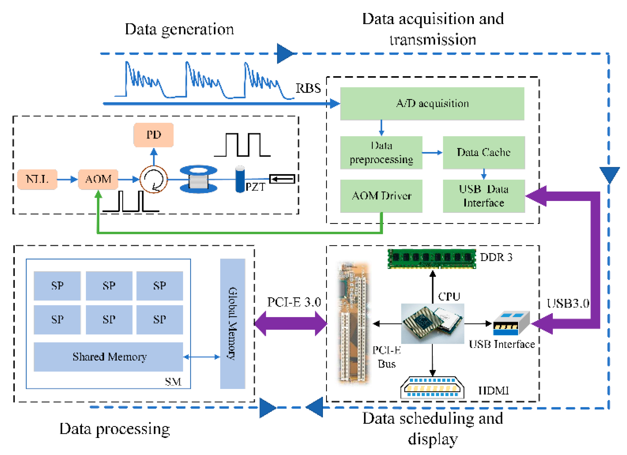
In our experiment, the external disturbance acting on the sensing optical fiber is simulated by a PZT phase modulator whose acting length is 1.5 m and driving voltage is 10 Vpp. The PZT phase modulator acts, at a position of 1000 m, as the single-point vibration source in sinusoidal form with a frequency of 100 Hz, while the total length of the optical fiber is 2020 m. Thus, the number of effective sampling points is reduced to 1010 for one RBS curve, and the data volume of each effective RBS curve is 1.01 kB. With the repetition frequency of optical pulses of 8 kHz, the total number of RBS curves is 8000 in 1 s, and the effective data volume is 8.08 MB during an acquisition time of 1 s. The data is then sent to the USB port of the upper computer via the USB 3.0 transmission bus at a speed of 100 MB/s, so the minimum data transmission time is about 80.8 ms. Moreover, in the interior of the upper computer, the USB port is connected with a south bridge USB I/O interface chip through the I/O bus, and the USB I/O interface chip is linked with a north bridge chipset via the Peripheral Component Interconnect (PCI) bus. The north bridge chipset is responsible for communication with the Dynamic Random Access Memory (DRAM), Cache and CPU through the memory bus and the front side bus. As a result, the data transmission time in the interior of the upper computer is hard to calculate accurately because of its complexity, but the data transmission time between the upper computer and lower computer could be considered as a fixed value if the experimental parameters do not change.

Figure 6a shows the superposition of the first 100 consecutive RBS traces and the enlarged plot at the single vibration position of 1000 m. It can be clearly seen that the RBS curves evidently fluctuate in the range from 1000 to 1020 m, which corresponds to the spatial resolution of 20 m. However, the RBS curves remain stable within the other range. Figure 6b shows a two-dimensional time–distance RBS figure, with the X-axis being time and the Y-axis being distance. The evolution of the time verifies that the RBS curves remain stable outside the vibration area. This result verifies the feasibility of vibration detection and location by the Φ-OTDR sensing system.

4.1. Differential Accumulation Algorithm

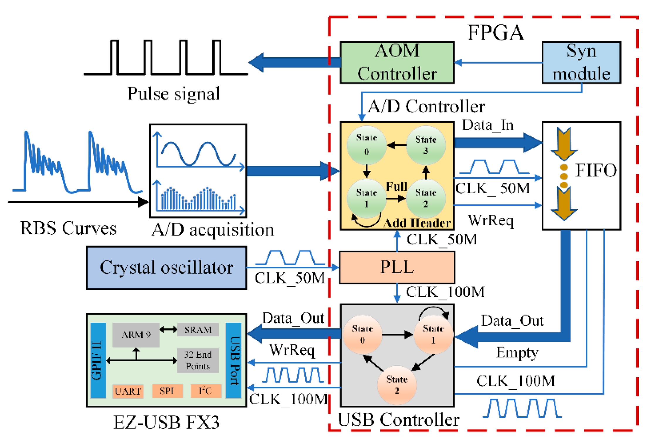
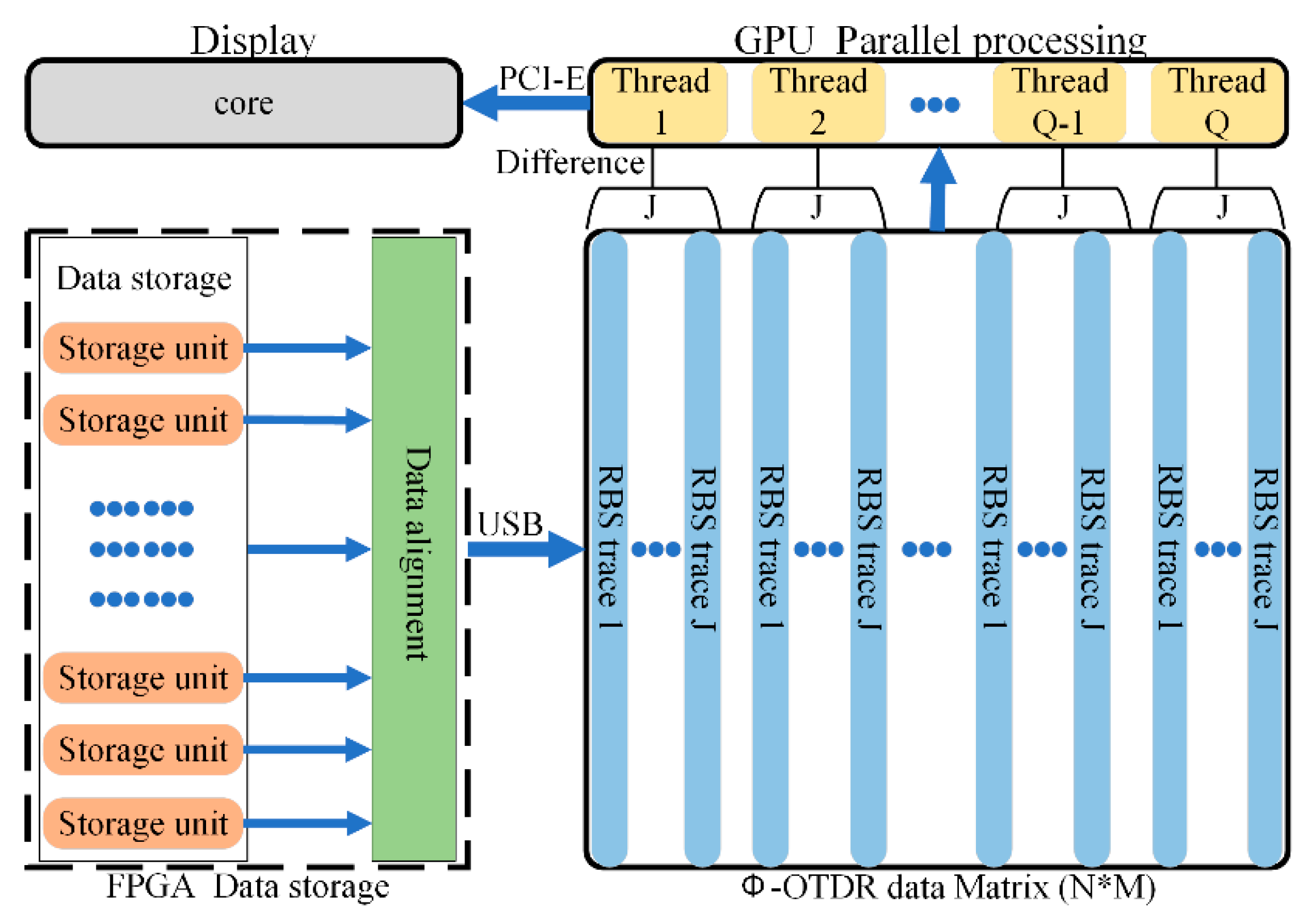
A differential accumulation algorithm is the conventional data processing method for a Φ-OTDR sensing system in order to realize the vibration location. It can remove the background noise and improve the signal-to-noise ratio (SNR). The cooperative data processing of differential accumulation algorithms with FPGA, CPU, and GPU is shown in Figure 7. The collected data in the storage unit goes through data alignment by the FPGA, which adds the data header before each RBS data string, and is then sent to the host computer via the USB transmission bus.

The received data is stored as the N*M matrix in the RAM of the host computer, which can be read and modified by the CPU. More concretely, the data matrix has M RBS curves, and there are N points in each RBS trace. Then, the data should be transmitted to the GPU via the Peripheral Component Interconnect-Express (PCI-E) bus. The differential accumulation processing of RBS traces is executed in the form of multiple threads in the GPU. For a differential accumulation algorithm, this only involves the simple calculation, multiplication and division, addition and subtraction functions. Therefore, this algorithm complexity is O(1).

The algorithm with multiple threads is shown in equations as follows:

$$dif{f}_{threadi,j}\left(n\right)=curv{e}_{j+k}\left(n\right)-curv{e}_j\left(n\right)$$

(3)

$$avg\left(n\right)=\frac{1}{Q}\frac{1}{J-k}{\displaystyle \sum _{threadi=1}^Q{\displaystyle \sum _{j=1}^{J-k}dif{f}_{threadi,j}\left(n\right)}}$$

(4)

where the order number of curves is j = 1, 2, 3, …, J − k, J is the number of curves in a thread, and k is the curve number between two subtractive curves. Then the order number of points in one curve is n = 1, 2, 3, …, N, and the length of each RBS curve is N. Then, the order number of threads is marked as threadi = 1, 2, 3, …, Q, and the total number of threads is represented as Q. Therefore, Q multiplied by J is M.

Equation (3) means the subtraction of the RBS curves with an interval of k in one thread and the J − k curves could be thus obtained in one thread. Because of the function of parallel computing, each thread could execute the instruction of Equation (3) at the same time.

In Equation (4), the differential data in one thread is accumulated and averaged, and each thread performs this operation in parallel. Therefore, each thread generates an average curve which contains N points, and Q curves can be obtained in total. Then, these Q curves are accumulated and averaged again in one thread to obtain a final vibration positioning curve, which can be sent to the display unit controlled by the CPU.

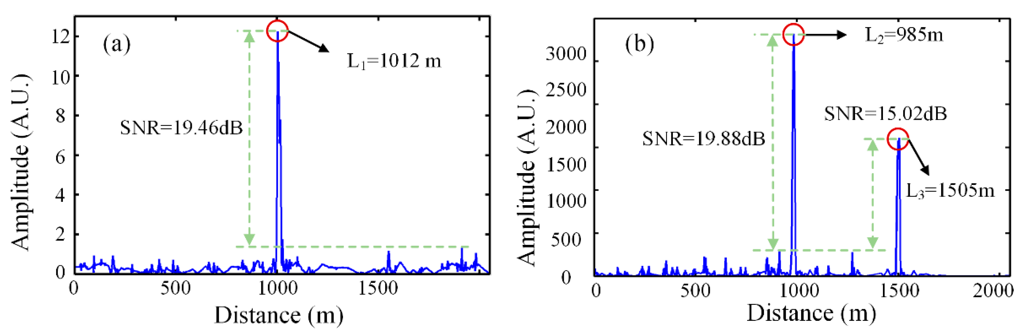
Figure 8 demonstrates the positioning results of differential accumulation algorithm for 2000 RBS curves and the interval value of k in Equations (3) and (4) is chosen as five in this experiment. Figure 8a shows the single-point vibration positioning result. The external disturbance is located at 1012 m, with a positioning error of 12 m and SNR of 19.46 dB while the total length of optical fiber is 2020 m. Figure 8b shows the multi-point vibration positioning result. The real disturbances are placed at 995 m and 1513 m away from the head of sensing optical fiber. The positioning results show that the first vibration position is at 985 m with an error of 10 m and SNR of 19.88 dB, and the second vibration position is at 1505 m with an error of 8 m and SNR of 15.02 dB, while the total length of optical fiber is 2036 m. So, the vibration position can be precisely located and has a high SNR by implementing a differential accumulation algorithm with the parallel computing of the GPU.

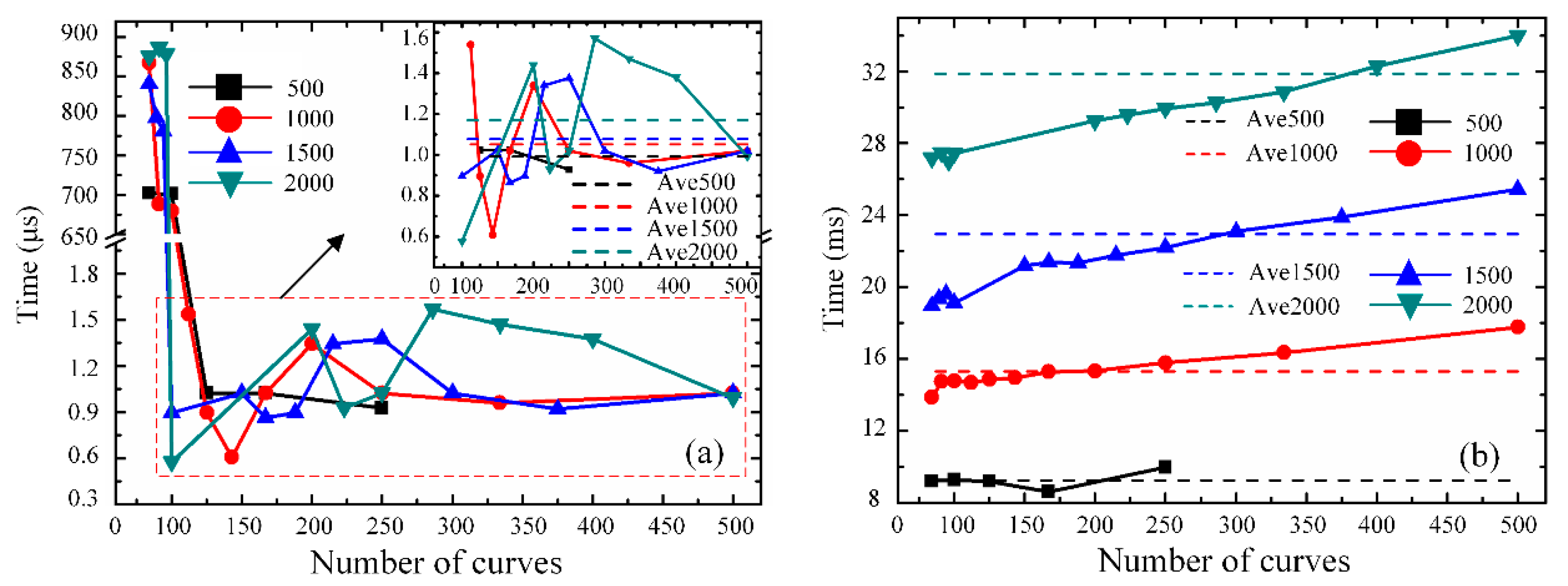
Furthermore, Figure 9 illustrates the time consumption comparison results for the differential accumulation processing of single-point vibration positioning between the GPU and CPU. The total number of RBS curves, which is denoted as M, is chosen as 500 (marked in black), 1000 (marked in red), 1500 (marked in blue) and 2000 (marked in green) in the comparison analysis.

Figure 9a shows the variation in time consumption of the differential accumulation calculations with the augmentation of the number of RBS curves in one thread on the GPU, when the differential accumulation is executed on the parallel computing platform. The X-axis represents the number of RBS curves in a thread (J), for a fixed number of all RBS curves (M = 500, 1000, 1500, 2000), the corresponding total number of threads (Q) could be also obtained by Q = M/J. For example, in Figure 9a, when the number of all RBS curves (M) is 2000, for the X-axis value (J) of 100, the total number of threads (Q) is 20.

It can be concluded that, when the value of J is less than 100 (which means that Q is more than 20), the time consumption is longer than 650 μs. This phenomenon may be explained by thread synchronization in the operation process of the GPU. The smaller value of J means the greater number of threads, which will lead to frequent thread switching on the GPU. The process of thread switching will also consume time, thus slow down the calculation time of the threads.

When the value of J is greater than 100 (which means that Q is less than 20), the variation in time consumption is specifically shown in the enlarged plot. The time consumption is largely reduced to less than 2 μs. As the number of curves in one thread increases, the time consumption shows the trend of irregular fluctuation. It demonstrates that the time consumption of differential accumulation algorithm computed on the GPU may be limited by many factors, which are not only related to the number of RBS curves, but also may be influenced by the thread cache or the thread switch process.

Moreover, the change in the GPU type may increase the number of threads, but the number of threads is not the only factor affecting the computing capabilities of the system. The computing capability of the Φ-OTDR system depends not only on the number of allocated threads, but also on the amount of sensing data. Because of the thread cache allocation, or the thread switching process, in the GPU, these factors will also affect the computing capability of the system. Therefore, the algorithm complexity, the amount of sensing data and the number of threads all need to be considered for the system optimization.

Figure 9b illustrates the variation in time consumption of the differential accumulation algorithm with serial computing based on the CPU. When the total number of RBS curves is fixed, a conclusion can be drawn—that the time gradually increases with the rising number of curves in a serial computing process. In addition, when the total number of RBS curves increases, the average time rises correspondingly, which is also marked by the short straight lines.

By comparing Figure 9a with Figure 9b, when the total number of RBS curves is same, the processing time of parallel operations based on the GPU is far less than that of serial computations based on the CPU. For the differential accumulation algorithm, when the length of optical fiber is 2020 m and the number of processed curves is 2000, the time spent on the GPU is only 1.6 μs. Under the same conditions, the CPU takes about 34 ms to realize data processing. It can be demonstrated that the method of combining the GPU and CPU is faster than serial computing architecture based on the CPU in relation to the differential accumulation algorithm for a Φ-OTDR vibration sensing system. Therefore, GPU can speed up the data processing of a differential accumulation algorithm and improve the real-time performance of a Φ-OTDR sensing system.

4.2. FFT Analysis Processing

Figure 10 shows the cooperation process of the CPU and GPU to realize the spectrum analysis, which could be important for the position location and frequency component analysis of the external disturbance. Firstly, the original Φ-OTDR data acquired by FPGA is transferred into the RAM of the host computer via the USB bus, and can then be processed in the form of the Φ-OTDR data matrix (N*M), with N time traces and M sampling points in each time trace. Secondly, the CPU copies time traces into graphics memory, which can be read and modified by the GPU through the memory copy function. The GPU then allocates simultaneously numerous threads to achieve the one-dimensional FFT computation. In addition, n represents the number of time traces in a thread on the GPU.

Finally, the processed result is sent back to the host computer via the PCI-E bus and is displayed on the screen. Thus, the frequency spectrum of temporal signal can be obtained, and it is beneficial to identify the external vibration position. In conclusion, this parallel operating method largely shortens the data processing time compared with the traditional serial computing method based on the CPU.

The process of FFT analysis based on the GPU mainly contains two parts, which are multiple curves parallel computation and the butterfly operation, which relies on the butterfly-shaped arithmetic unit. It can simultaneously provide the needed operands for many arithmetic units, owing to the advantages of its parallel structure and in-place calculation. Thus, this parallel operation structure improves the speed of FFT calculation and shortens the time noticeably. Because of the butterfly operation of FFT, when the number of calculation points is M in one curve, the algorithm complexity is O(M/2 × log2(M)).

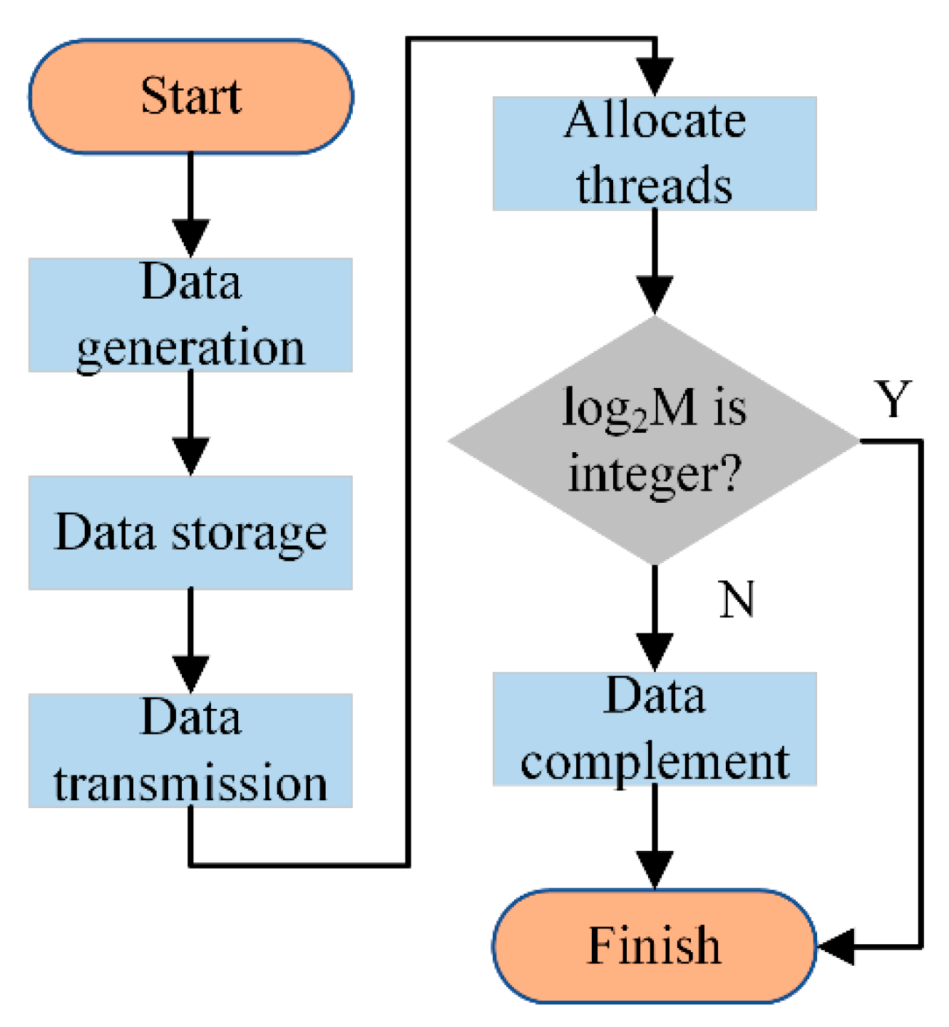
The process of the first part is shown in Figure 11, the RBS data is generated and stored in the CPU and transmitted into the GPU. Then, the N threads are allocated for the time traces, which means each time curve is processed by one thread. It is necessary to verify whether the length of the time trace (M) is a power of two, owing to the existence of the butterfly operation. If the length is not a power of two, the data needs to be complemented by adding a zero value at the end of the data string. Each curve is processed by these steps on the GPU at the same time.

The second part is the butterfly operation of each time trace by using the butterfly arithmetic unit. This FFT analysis is called decimation in time (DIT) FFT. The process is shown in the equation as follows:

$$X\left(k\right)=DFT\left[x\left(n\right)\right]={\displaystyle \sum _{n=0}^{M-1}x\left(n\right)}{W}_M^{kn}\begin{array}{cc}& \end{array}0\le k\le M-1$$

(5)

Equation (5) represents the computation process of conventional discrete Fourier transform (DFT). In Equation (5), $W_M^{\mathrm{kn}}$ is the rotation factor which has features of symmetry and periodicity. This characteristic can decrease the computation time of FFT. The signal of the temporal domain (x(n)) could be decomposed into even and odd sequences, so the FFT of the even data sequence is called as X₁(k) and the FFT of the odd data sequence is called as X₂(k). It is shown in the equation as follows:

$$\begin{array}{l}{X}_1\left(k\right)={\displaystyle \sum _{n=0}^{\raisebox{1ex}{$M$}\!\left/ \!\raisebox{-1ex}{$2$}\right.-1}x\left(2n\right)}{W}_{\raisebox{1ex}{$M$}\!\left/ \!\raisebox{-1ex}{$2$}\right.}^{\mathrm{nk}}\\ X_2\left(k\right)={\displaystyle \sum _{n=0}^{\raisebox{1ex}{$M$}\!\left/ \!\raisebox{-1ex}{$2$}\right.-1}x\left(2n+1\right)}{W}_{\raisebox{1ex}{$M$}\!\left/ \!\raisebox{-1ex}{$2$}\right.}^{\mathrm{nk}}\end{array}$$

(6)

Therefore, Equation (5) could be developed as Equation (7).

$$\begin{array}{l}{X}_{threadi}\left(k\right)=X_1\left(k\right)+W_M^k{X}_2\left(k\right)\\ X_{threadi}\left(k+\raisebox{1ex}{$M$}\!\left/ \!\raisebox{-1ex}{$2$}\right.\right)=X_1\left(k\right)-W_M^k{X}_2\left(k\right)\begin{array}{cc}& \end{array}0\le k\le \raisebox{1ex}{$M$}\!\left/ \!\raisebox{-1ex}{$2$}\right.-1\end{array}$$

(7)

Equation (7) expresses the principle of the butterfly operation in one thread. X_threadi(k) indicates the frequency value of the first half of all points and X_threadi (k + M/2) indicates the frequency value of the second half of all points. Then, the order of threads is marked as threadi = 1, 2, 3, …, Q, and the total number of threads is represented as Q.

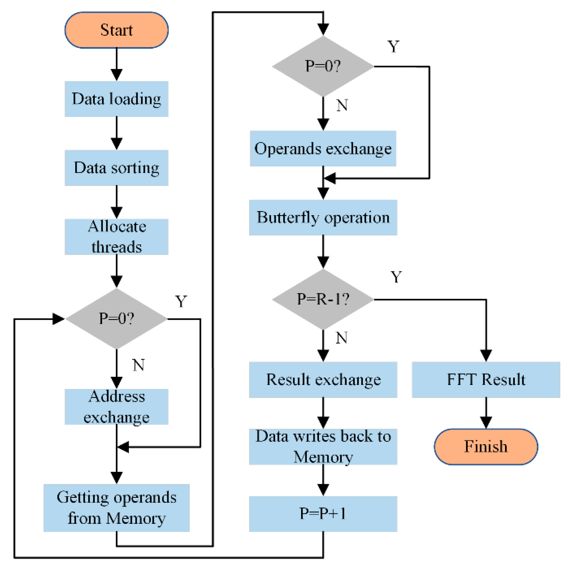
The FFT analysis process is shown in Figure 12. The data value of each time trace is needs to be sorted before processing by the butterfly arithmetic unit. Firstly, the natural sequence number of x(n) in Equation (5) is transformed and expressed in the binary form. Then, the corresponding binary number is flipped. Afterwards, these sequence numbers are converted to the decimal label. Therefore, x(n) is sorted and stored in the memory in the new numerical order.

FFT computation of M data points is achieved by using an R-level butterfly operation with R = log₂M; each level has an M/2 arithmetic unit to perform the butterfly operation at the same time. The current level number of butterfly computation is denoted as P, P = 0, 1, 2, …, R − 1.

From Figure 12, each butterfly computation is achieved by one thread, and M/2 threads are allocated to a time trace which contains M points. There are three kinds of exchange operations in the FFT process based on the principle of in-place computation, which are the address exchange, the operands exchange, and the results exchange after the butterfly operation. The zero-level butterfly computation only performed one exchange operation, which is the result exchange after a butterfly operation. When the value of P is not equal to zero, the obtained frequency values will replace previous frequency values. However, the (R − 1)-level butterfly computation only realizes two exchange operations, which are the address exchange and the operands exchange.

DIT FFT has the characteristic of in-place computation. It means that the output data of the same butterfly arithmetic unit will replace the position of the input data in the memory space. In addition, every butterfly arithmetic unit of same level operates independently, which provides the theory basis for the multi-thread processor on the GPU. Every thread executes a butterfly arithmetic unit, but the processing data in the thread will refresh with the growing number of butterfly operator levels. Therefore, it can largely decrease computational complexity and the storage space of data. Essentially, applying DIT FFT on the GPU can speed up data processing. Eventually, the real-time performance of the Φ-OTDR sensing system could be improved.

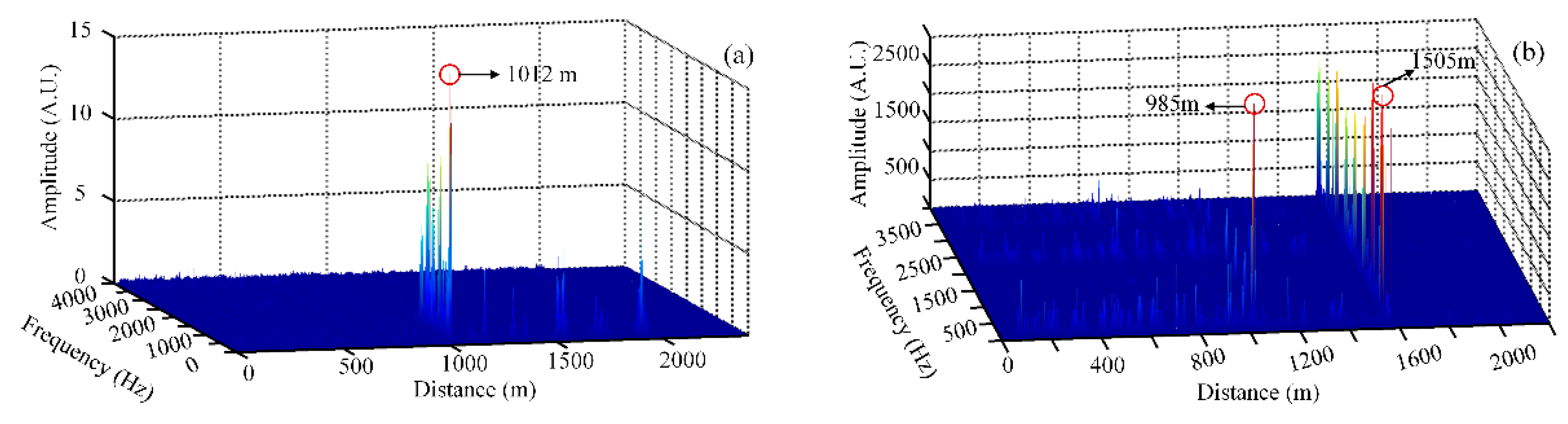
In our experiment system, a single-point vibration test at a position of 1000 m is applied, while the total length of optical fiber is 2020 m. A two-points vibration test at the positions of 995 m and 1513 m are applied, while the total length of optical fiber is 2036 m. Each time trace contains 1024 points. All time-series curves are dealt with FFT processing with a frequency resolution of 7.80 Hz on the GPU, and the obtained frequency–space waterfall map is shown in Figure 13. From Figure 13a, the exerted external vibration is detected and located at a position of 1012 m, and the location error is 12 m. From Figure 13b, the vibration is exerted on two positions of 985 and 1505 m. The location errors are, thus, 10 and 8 m.

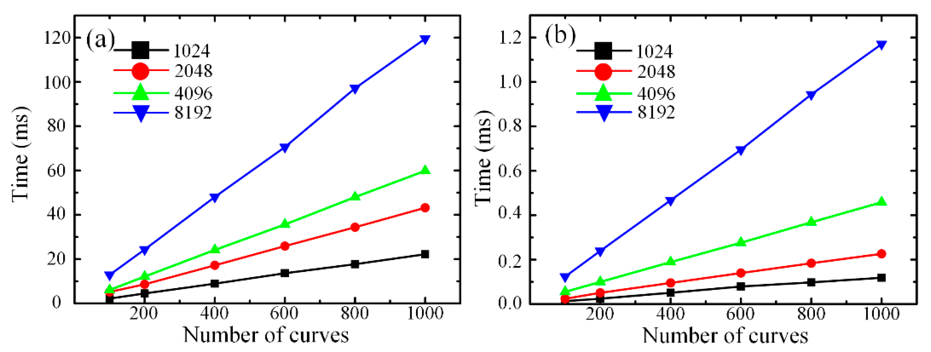
Figure 14 illustrates the computing time contrast of FFT analysis processing on the CPU and GPU. The abscissae of Figure 14a,b represent the number of time curves, which positively correlate with the length of optical fiber. The ordinate means the computing time of the data analysis.

From Figure 14a,b, when the length of optical fiber is changeless, with the growing number of points which needs to be executed for FFT analysis processing, the time increases gradually as well. When the number of points is constant, the time shows the trend linearly rising with the growing length of optical fiber. Comparing Figure 14a with Figure 14b, it can be concluded that the computing time of FFT operation based on the CPU is much longer than that based on the GPU when the point number of FFT analysis and the length of optical fiber is invariable. When the length of optical fiber is 2020 m and the point number of FFT is 8192, the consumption time is 1.17 ms with FFT analysis performed on the GPU. Under this experimental condition, it takes about 119.5 ms with FFT analysis performed on the CPU, so the speed of using GPU is approximately 140 times faster than that of traditional series computation based on a CPU in FFT analysis processing. It can be noted that a parallel computation method based on the GPU can shorten substantially the time of FFT analysis processing and optimize the real-time performance of the Φ-OTDR sensing system.

4.3. Extended Comparison Experiments and Discussions

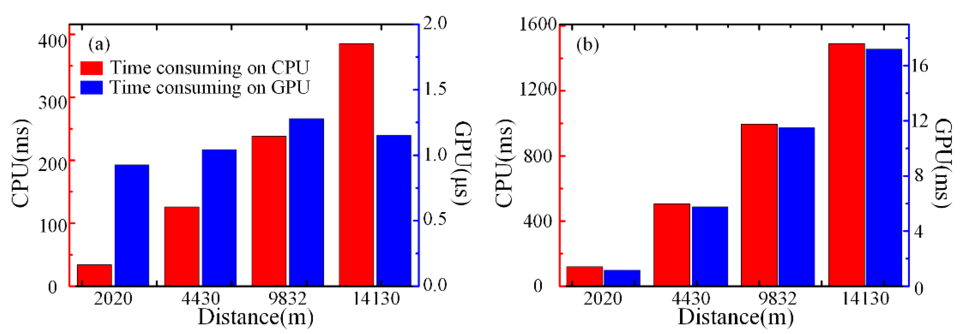
In addition, we also did the experiment in long distance conditions to verify the feasibility and effectiveness of our parallel computation method based on the GPU. The lengths of optical fiber are 2020, 4430, 9832 and 14,130 m, respectively. The differential accumulation algorithm and the FFT processing both are executed on the CPU and GPU. The experiment results are shown in Figure 15.

The time contrast between the CPU and GPU for the differential accumulation algorithm is shown in Figure 15a when the number of RBS curves is 2000. The red bar chart shows the time consumed on the CPU, and the longer the distance, the longer the time consumed. The blue bar chart shows the time consumed on the GPU. The changing trend of time is not regular, but floats up and down with the microsecond level. This phenomenon demonstrates that the time consumption of the differential accumulation algorithm on the GPU may be limited by many factors, which is not only related to the optical fiber distance, but also may be influenced by the thread cache allocation or the thread switching process in the GPU, which also has an uncertain time consumption less or close to one microsecond. In the condition of the same amount of data, the time spent on the GPU is far less than that of the CPU. It can be demonstrated that the method of combining the GPU and CPU can realize fast data processing in relation to the differential accumulation algorithm for a Φ-OTDR vibration sensing system.

The time contrast between the CPU and GPU for FFT processing is shown in Figure 15b when the point number of FFT is 8192. The red and blue bar chart represents the time consumption of FFT processing on the CPU and GPU, respectively. With the increase in distance, both CPU and GPU show the same trend of growth. Moreover, in the condition of same amount of data, the time spent on the CPU is 100 times more than that of the GPU. It demonstrates that our parallel computation based on the GPU can shorten substantially the time of FFT analysis processing and optimize the real-time performance of the Φ-OTDR sensing system.

Evidently, the feasibility and validity of our parallel computation method based on the GPU are verified under long distance and large data volume conditions for the differential accumulation algorithm and FFT processing. Therefore, this paper verifies that the distributed optical fiber sensor is another example of a GPU application. Because of the large amount of sensing data and real-time performance requirement in practical applications of distributed optical fiber sensors, the GPU is used as an effective solution to improve the speed of data processing with a strong parallel computing capability.

Based on the above discussion, the differential accumulation algorithm and FFT processing on the GPU could lead to less time being consumed. However, the use of the GPU will also bring the problem of increasing cost. Therefore, the identification of when the GPU will be necessary for real-time operation could be our next research direction. In this study, we only put forward a preliminary mathematical criterion which could be optimized for real application in the GPU.

In the experimental setup, the maximum real-time data throughput is 100 MB/s and the data acquisition speed is 50 MSa/s. If each sampling point is set to be represented by 8 bits (1 Byte), the acquisition time (T_a) and the transmission time (T_t) could be simplified as T_a = 2 s and T_t = 1 s for the same data volume of 100 MB. Thus, the time consumed in the lower system (T_ls), including the FPGA board and the PCI-E bus, could be considered as T_ls = max(T_a, T_t) = 2 s.

Meanwhile, considering the complexity of the algorithm, FFT processing consumes more time. Based on the linear relationship in Figure 14, the time consumed by FFT processing on the CPU (T_CPU) and GPU (T_GPU) is T_CPU = 120 ms and T_GPU = 1.2 ms while the point number of FFT processing is 8192 and the number of RBS curves is 1000. Thus, the time consumed could be calculated as T_CPU = 1920 ms and T_GPU = 19.2 ms if the number of RBS curves (N_RBS) N_RBS = 16,000 with the repetition frequency of optical pulses of 8kHz in our experimental setup. Considering that the CPU also needs memory allocation, reading and writing operations, the time consumed in the upper system (T_us), including the CPU and internal bus, should be greater than T_CPU, which means that T_us = kT_CPU with the coefficient k > 1.

As a result, if T_us > T_ls, which means kT_CPU > max(T_a, T_t), it is recommended to use the GPU to optimize the execution time of the processing algorithm. By contrast, if T_us < T_ls, which means kT_CPU < max(T_a, T_t), the use of the CPU may be also acceptable.

5. Conclusions

In this paper, the feasibility of speeding up the data processing rate of the Φ-OTDR sensing system by using the method of cooperation between the CPU and GPU processing is discussed and experimentally verified. Two typical signal processing methods for the Φ-OTDR sensing system are realized in parallel operations based on the GPU and traditional serial computations based on the CPU, respectively. For the differential accumulation algorithm which can achieve vibration detection and location, serial computations only based on the CPU take about 21,250 times as much execution time as parallel operations in the condition of same data volume. Thus, the GPU greatly accelerates the processing speed of the differential accumulation algorithm for the Φ-OTDR sensing system. For the FFT analysis which can precisely achieve vibration location and spectrum analysis, the computation time with the GPU is approximately 140 times faster than serial computation under same experimental condition. It shows that the GPU can effectively improve the FFT processing speed of the Φ-OTDR sensing system. In addition, the fast data collection and transmission are achieved by using data acquisition system based on FPGA. In conclusion, this novel data co-processing parallel computation method, which combines FPGA technology with the CPU and GPU accelerator, can realize data acquisition, transmission, and processing in parallel, and eventually optimize the real-time performance of the Φ-OTDR sensing system.

In this paper, we use the underlying CUDA API to realize multi-thread parallel computing in the GPU for distributed optical fiber sensors; this function encapsulation may become a research direction for embedded and portable application requirements, with the challenges of function optimization and algorithm simplification. In addition, in order to improve the processing speed of the whole system, collaborative parallel research into multi-processors will be a potential research direction. For example, further research on the parallel operations of several CPUs or several GPUs may be conducted, which could promote the parallel operation of a data processing algorithm in a Φ-OTDR system. Therefore, multi-processors may be a parallel operation solution for the academic and industry communities.

References

1. Zhang, Y.X.; Xu, Y.M.; Shan, Y.Y.; Sun, Z.H.; Zhu, F.; Zhang, X.P. Polarization dependence of phase-sensitive optical time-domain reflectometry and its suppression method based on orthogonal-state of polarization pulse pair. Opt. Eng. 2016, 55, 074109. [Google Scholar] [CrossRef]
2. He, H.J.; Shao, L.Y.; Li, Z.L.; Zhang, Z.Y.; Zou, X.H.; Luo, B.; Pan, W.; Yan, L.S. Self-Mixing demodulation for coherent phase-sensitive OTDR system. Sensors 2016, 16, 681. [Google Scholar] [CrossRef] [PubMed]
3. Hui, X.N.; Zheng, S.L.; Zhou, J.H.; Chi, H.; Jin, X.F.; Zhang, X.M. Hilbert-Huang transform time-frequency analysis in phi-OTDR distributed sensor. IEEE Photon. Technol. Lett. 2014, 26, 2403–2406. [Google Scholar] [CrossRef]
4. Wang, Y.; Yuan, H.Y.; Liu, X.; Bai, Q.; Zhang, H.J.; Gao, Y.; Jin, B.Q. A Comprehensive Study of Optical Fiber Acoustic Sensing. IEEE Access 2019, 7, 85821–85837. [Google Scholar] [CrossRef]
5. Wang, Y.; Wang, P.F.; Ding, K.; Li, H.; Zhang, J.G.; Liu, X.; Bai, Q.; Wang, D.; Jin, B.Q. Pattern recognition using relevant vector machine in optical fiber vibration sensing system. IEEE Access 2019, 7, 5886–5895. [Google Scholar] [CrossRef]
6. Tejedor, J.; Martins, H.F.; Piote, D.; Macias-Guarasa, J.; Pastor-Graells, J.; Martin-Lopez, S.; Corredera Guillen, P.; De Smet, F.; Postvoll, W.; Gonzalez-Herraez, M. Toward prevention of pipeline integrity threats using a smart fiber-optic surveillance system. J. Lightw. Technol. 2016, 34, 4445–4453. [Google Scholar] [CrossRef] [Green Version]
7. Fan, X.Y.; Yang, G.Y.; Wang, S.; Liu, Q.W.; He, Z.Y. Distributed fiber-optic vibration sensing based on phase extraction from optical reflectometry. J. Lightw. Technol. 2017, 35, 3281–3288. [Google Scholar] [CrossRef]
8. Peng, F.; Wu, H.; Jia, X.H.; Rao, Y.J.; Wang, Z.N.; Peng, Z.P. Ultra-long high-sensitivity phi-OTDR for high spatial resolution intrusion detection of pipelines. Opt. Exp. 2014, 22, 13804–13810. [Google Scholar] [CrossRef]
9. Song, M.P.; Zhu, W.J.; Xia, Q.L.; Yin, C.; Lu, Y.; Wu, Y.; Zhuang, S.W. 151-km single-end phase-sensitive optical time-domain reflectometer assisted by optical repeater. Opt. Eng. 2018, 57, 027104. [Google Scholar] [CrossRef]
10. Shi, Y.; Feng, H.; Zeng, Z.M. A long distance phase-sensitive optical time domain reflectometer with simple structure and high locating accuracy. Sensors 2015, 15, 21957–21970. [Google Scholar] [CrossRef] [Green Version]
11. Qin, Z.G.; Chen, L.A.; Bao, X.Y. Wavelet denoising method for improving detection performance of distributed vibration sensor. IEEE Photon. Technol. Lett. 2012, 24, 542–544. [Google Scholar] [CrossRef]
12. Lu, Y.L.; Zhu, T.; Chen, L.A.; Bao, X.Y. Distributed vibration sensor based on coherent detection of phase-OTDR. J. Lightw. Technol. 2010, 28, 3243–3249. [Google Scholar]
13. Yang, A.; Feng, X.; Li, J.; Feng, H.; Jin, S.J. Two-beam phase-sensitive optical time domain reflectometer based on Jones matrix modeling. Opt. Eng. 2013, 52, 094102. [Google Scholar]
14. Martins, H.F.; Martin-Lopez, S.; Corredera, P.; Filograno, M.L.; Frazão, O.; González-Herráez, M. High visibility phase-sensitive optical time domain reflectometer for distributed sensing of ultrasonic waves. In Proceedings of the Fifth European Workshop on Optical Fibre Sensors, Krakow, Poland, 19–22 May 2013. [Google Scholar]
15. Yue, H.M.; Zhang, B.; Wu, Y.X.; Zhao, B.Y.; Li, J.F.; Ou, Z.H.; Liu, Y. Simultaneous and signal-to-noise ratio enhancement extraction of vibration location and frequency information in phase-sensitive optical time domain reflectometry distributed sensing system. Opt. Eng. 2015, 54, 047101. [Google Scholar] [CrossRef]
16. Yu, M.; Liu, M.H.; Chang, T.Y.; Lang, J.P.; Chen, J.D.; Cui, H.L. Phase-sensitive optical time-domain reflectometric system based on a single-source dual heterodyne detection scheme. Appl. Opt. 2017, 56, 4058–4064. [Google Scholar] [CrossRef]
17. Liu, X.; Wang, Y.; Wu, R.D.; Wang, D.; Bai, Q.; Jin, B.Q. Real-Time phase-sensitive OTDR based on data matrix matching method. Sensors 2018, 18, 1883. [Google Scholar] [CrossRef] [Green Version]
18. Navarro, C.A.; Hitschfeld-Kahler, N.; Mateu, L. A survey on parallel computing and its applications in data-parallel problems using GPU architectures. Commun. Comput. Phys. 2014, 15, 285–329. [Google Scholar] [CrossRef] [Green Version]
19. Cao, W.; Xu, C.F.; Wang, Z.H.; Yao, L.; Liu, H.Y. CPU/GPU computing for a multi-block structured grid based high-order flow solver on a large heterogeneous system. Clust. Comput. 2014, 17, 255–270. [Google Scholar] [CrossRef]
20. Gropp, W.; Snir, M. Programming for exascale computers. Comput. Sci. Eng. 2013, 15, 27–35. [Google Scholar] [CrossRef] [Green Version]
21. Hui, X.N.; Ye, T.H.; Zheng, S.L.; Zhou, J.H.; Chi, H.; Jin, X.F.; Zhang, X.M. Space-frequency analysis with parallel computing in a phase-sensitive optical time-domain reflectometer distributed sensor. Appl. Opt. 2014, 53, 6586–6590. [Google Scholar] [CrossRef]
22. Sha, Z.; Feng, H.; Shi, Y.; Zeng, Z.M. Phase-sensitive optical time domain reflectometer with ultrafast data processing based on GPU parallel computation. Appl. Opt. 2018, 57, 2679–2685. [Google Scholar] [CrossRef] [PubMed]
23. Razak, A.A.; Yokota, M. Transmission properties of Fiber Bragg Grating with GPU support. In Proceedings of the IEEE International Conference on Computational Electromagnetics (ICCEM), Kumamoto, Japan, 8–10 March 2017. [Google Scholar]
24. Sanchez-Lara, R.; Trejo-Sanchez, J.A.; Lopez-Martinez, J.L.; Alvarez-Chavez, J.A. Simulation of an inelastic dispersive phenomenon: Stimulated Brillouin scattering in a single-mode fiber segment through parallelism. J. Supercomput. 2018, 74, 3264–3277. [Google Scholar] [CrossRef]
25. Kockara, S.; Halic, T.; Bayrak, C. Real-time minute change detection on GPU for cellular and remote sensor imaging. In Proceedings of the 23rd International Conference on Advanced Information Networking and Applications Workshops, Bradford, England, 26–29 May 2009. [Google Scholar]
26. Homm, F.; Kaempchen, N.; Ota, J.; Burschka, D. Efficient occupancy grid computation on the GPU with lidar and radar for road boundary detection. In Proceedings of the IEEE Intelligent Vehicles Symposium (IV), San Diego, CA, USA, 21–24 June 2010. [Google Scholar]
27. Monmasson, E.; Idkhajine, L.; Cirstea, M.N.; Bahri, I.; Tisan, A.; Naouar, M.W. FPGAs in industrial control applications. IEEE Trans. Ind. Inf. 2011, 7, 224–243. [Google Scholar] [CrossRef] [Green Version]
28. HajiRassouliha, A.; Taberner, A.J.; Nash, M.P.; Nielsen, P.M.F. Suitability of recent hardware accelerators (DSPs, FPGAs, and GPUs) for computer vision and image processing algorithms. Signal Process. Image Commun. 2018, 68, 101–119. [Google Scholar] [CrossRef]
29. Lei, J.; Li, D.L.; Zhou, Y.L.; Liu, W. Optimization and acceleration of flow simulations for CFD on CPU/GPU architecture. J. Braz. Soc. Mech. Sci. 2019, 41, 290. [Google Scholar] [CrossRef]
30. Lindholm, E.; Nickolls, J.; Oberman, S.; Montrym, J. NVIDIA Tesla: A unified graphics and computing architecture. IEEE Micro 2008, 28, 39–55. [Google Scholar] [CrossRef]
31. Nickolls, J.; Dally, W.J. The GPU computing era. IEEE Micro 2010, 30, 56–69. [Google Scholar] [CrossRef]
32. Ashraf, I.; Khammassi, N.; Taouil, M.; Bertels, K. Memory and Communication Profiling for Accelerator-based Platforms. IEEE Trans. Comput. 2018, 67, 934–948. [Google Scholar] [CrossRef]
33. Li, Q.; Zhang, C.X.; Li, L.J.; Zhong, X. Localization mechanisms and location methods of the disturbance sensor based on phase-sensitive OTDR. Optik 2014, 125, 2099–2103. [Google Scholar] [CrossRef]
34. Bracewell, R.N. The Fourier Transform and Its Applications, 3nd ed.; McGraw-Hill: New York, NY, USA, 1964; pp. 258–285. [Google Scholar]
35. Hlawatsch, F.; Boudreaux-Bartels, G.F. Linear and quadratic time-frequency signal representations. IEEE Signal Proc. Mag. 1992, 9, 21–67. [Google Scholar] [CrossRef]
36. Zhang, X.J.; Chen, J.; González-Vila, Á.; Liu, F.; Liu, Y.K.; Li, K.W.; Guo, T. Twist sensor based on surface plasmon resonance excitation using two spectral combs in one tilted fiber Bragg grating. JOSA B 2019, 36, 1176–1182. [Google Scholar] [CrossRef]
Figure 1. Contrast diagram of field-programmable gate array (FPGA), central processing unit (CPU) and graphics processing unit (GPU) internal structure: (a) the internal structure of FPGA (b) the internal structure of CPU (c) the internal structure of GPU.
Applsci 10 01747 g001
Figure 2. The diagram of experiment setup.
Applsci 10 01747 g002
Figure 3. Data flow and storage analysis.
Applsci 10 01747 g003
Figure 4. Functions of FPGA in Φ-OTDR sensing system.
Applsci 10 01747 g004
Figure 5. The processing architecture of compute unified device architecture (CUDA).
Applsci 10 01747 g005
Figure 6. (a) The superposition of 100 Rayleigh backwards scattering (RBS) traces, (b) two-dimension time–distance RBS figure.
Applsci 10 01747 g006
Figure 7. Cooperative data processing with FPGA, GPU and CPU.
Applsci 10 01747 g007
Figure 8. Position curves after differential accumulation algorithm for (a) the single-point vibration position and (b) the multi-point vibration positions.
Applsci 10 01747 g008
Figure 9. The time consumption comparison results for the differential accumulation processing of single-point vibration positioning between the GPU and CPU: (a) the time spent on GPU (b) the time spent on CPU.
Applsci 10 01747 g009
Figure 10. Cooperative data processing with GPU and CPU.
Applsci 10 01747 g010
Figure 11. The data processing flow chart of time traces.
Applsci 10 01747 g011
Figure 12. The flow chart of fast Fourier transform (FFT) algorithm on GPU.
Applsci 10 01747 g012
Figure 13. The obtained frequency–space map after processed with GPU: (a) for single-point vibration (b) for two-points vibration.
Applsci 10 01747 g013
Figure 14. The time contrast of FFT processing on CPU and GPU: (a) the time spent on CPU (b) the time spent on GPU.
Applsci 10 01747 g014
Figure 15. The time contrast between CPU and GPU under different distances for (a) the differential accumulation algorithm and (b) the FFT processing.
Applsci 10 01747 g015