Deep Neural Network for Predicting Ore Production by Truck-Haulage Systems in Open-Pit Mines

Abstract

This paper proposes a deep neural network (DNN)-based method for predicting ore production by truck-haulage systems in open-pit mines. The proposed method utilizes two DNN models that are designed to predict ore production during the morning and afternoon haulage sessions, respectively. The configuration of the input nodes of the DNN models is based on truck-haulage conditions and corresponding operation times. To verify the efficacy of the proposed method, training data for the DNN models were generated by processing packet data collected over the two-month period December 2018 to January 2019. Subsequently, following training under different hidden-layer conditions, it was observed that the prediction accuracy of morning ore production was highest when the number of hidden layers and number of corresponding nodes were four and 50, respectively. The corresponding values of the determination coefficient and mean absolute percentage error (MAPE) were 0.99% and 4.78%, respectively. Further, the prediction accuracy of afternoon ore production was highest when the number of hidden layers was four and the corresponding number of nodes was 50. This yielded determination coefficient and MAPE values of 0.99% and 5.26%, respectively.

1. Introduction

In open-pit mines, ore loading and hauling material-handling operations account for approximately 50% of the total mine-operation cost [1]. Therefore, it is essential to design a truck-haulage system that not only maximizes mine productivity and equipment-management efficiency but also minimizes haulage cost [2]. Recently, several discrete-event simulation techniques [3,4,5,6,7,8,9,10,11] have been proposed for realizing effective truck-haulage systems designs. The allocation phase in the simulation of truck-haulage systems involves selecting the type, size, number, and payload of fleets suitable for use in haulage operations. This is followed by a dispatch phase that assigns trucks to a specific shovel by considering ore production and equipment utilization [12]. Several simulation algorithms based on mixed-integer linear programming [13,14,15], queuing theory [2,16,17,18,19], linear programming [20,21,22], goal programming [23], and stochastic programming [24] have been proposed for fleet allocation. Simulation techniques based on the assignment-problem [25,26] and transportation-problem [27] approaches have also been developed for truck dispatching. Several other products for sophisticating truck dispatching, such as Modular Mining Systems’ DISPATCH^® [28] and Caterpillar’s CAT^® MINESTAR ™ [29], have also been commercialized.

Information communication technologies (ICTs), such as wireless communications, sensor networks, global positioning system (GPS), and cloud computing, have been implemented at open-pit-mining sites to facilitate real-time monitoring of the operating status and haulage information of equipment, as well as collection of equipment-tracking data on web servers [30,31,32,33,34,35,36,37,38]. Further, several truck-dispatch techniques have been proposed to simulate truck systems using real-time data collected from mining sites. For example, Tan et al. [39] identified discrete haulage-operation events by analyzing historical GPS truck-tracking data and implemented a truck-dispatch simulation algorithm using the Arena^® software. Chaowasakoo et al. [40] developed a real-time truck-dispatch system that plans truck-haulage strategies using truck-shovel activity-time data obtained from GPS.

However, providing a comprehensive and effective truck-haulage systems simulation algorithm is difficult. First, open-pit mines are characterized by frequent changes in loading points during operations along with the use of multiple equipment-movement paths, unlike underground mines [1]. Additionally, several environmental factors, such as the weather, rock characteristics, and road conditions, affect haulage operations [12,41]. Thus, it is difficult to design a simulation algorithm for truck-haulage systems in large open-pit mines, where ore loading and haulage operations are simultaneously performed at multiple locations. Moreover, several types of simulation algorithms can be developed for a haulage plan that changes in real time, and it is difficult to alter these algorithms depending on variations in the haulage plan. Therefore, it is necessary to develop a simulation strategy that understands not only the characteristics of truck-haulage systems but also the sequence of discrete haulage operations. Additionally, the simulation technique must accurately predict ore production and equipment utilization using equipment-tracking data previously accumulated without use of prior-knowledge-based algorithms.

Deep learning methods have recently attracted increased research interest because they facilitate easy analysis and efficient processing of large amounts of big data obtained from ICT systems [42]. Deep learning is an artificial intelligence (AI) technique wherein a computer analyzes data characteristics and designs prediction models without human interference or prior knowledge [43]. Deep learning methods extract high-level data features by using models that comprise a hierarchical connection of the input, hidden, and output layers [44,45]. Nodes within each layer are connected to those in subsequent layers and provide predicted values as output using a feed-forward method. In this way, training of a deep learning model continues until prediction errors are minimized [46,47]. Deep learning models are classified into several types, such as a deep neural network (DNN) [45,46], convolutional neural network (CNN) [47,48], and recurrent neural network (RNN) [49,50], depending on the input-data type and data-processing method employed.

Recently, various investigations have been performed to incorporate deep learning techniques into mining-industry applications. Models that can detect anomalies [51,52,53], analyze deposit potential [54,55,56,57], predict fuel consumption by trucks [58], and recognize cutting patterns of coal-mining shearers [59] have been developed. Additionally, several risk-prediction systems employing deep learning techniques have been developed to prevent occurrence of mining accidents [60,61]. Other deep learning-based systems that have been recently developed include a visual object-detection system that can classify workers and heavy mining vehicles in open-pit mines [62], stability-evaluation system for gate roadways in a long wall-mining environment [63], and prediction system for health risks caused by whole body vibration of mining-truck drivers [64]. Baek and Choi [65] developed a DNN model to predict ore production and crusher utilization of a truck-haulage system using equipment-tracking data obtained using a wireless network system installed in an underground mine. However, no algorithm capable of learning truck-haulage-system characteristics and predicting ore production using equipment-tracking data has yet been developed for use in open-pit mining applications.

Predicting ore production through deep learning using equipment-tracking data affords several advantages. It aids comprehension of the operating patterns of haulage equipment and facilitates ore-production prediction exclusively using data obtained from mining sites without developing algorithms based on prior knowledge. Even in cases involving changes in the haulage plan, ore-production prediction can be realized by simply updating the prediction model with the latest datasets. Moreover, prediction of the latest ore produce can be realized by providing data obtained in real time as input to the prediction model. Furthermore, deep learning methods can be used throughout the lifetime of mines by continuously updating their underlying prediction model.

In this study, an open-pit limestone mine installed with an ICT-based mine-safety-management system was used as the investigation location. Two DNN models were designed to predict morning and afternoon ore productions, respectively, with the input-layer nodes of each model configured with the truck-haulage operating conditions and haulage-operation time as variables. DNN-model training data were generated by processing packet data collected over the two-month period December 2018 to January 2019. The two models were trained by varying the number of hidden layers and their corresponding nodes, and their prediction accuracy was evaluated by calculating the determination coefficient and mean absolute percentage error (MAPE) for the training and validation data. By using the DNN model with the lowest prediction error, morning and afternoon ore productions on five days of the second week of February 2019 were predicted and compared against observed values.

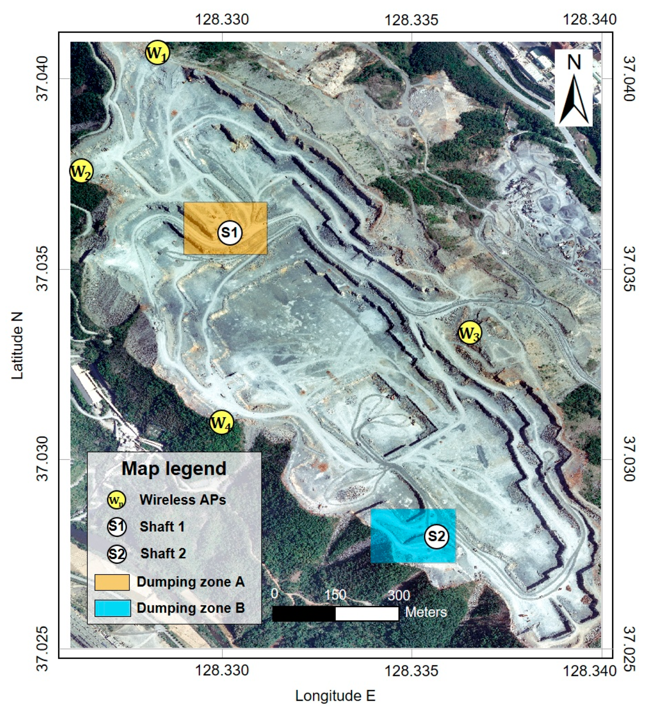
2. Study Area

In this study, an open-pit mine owned by Hanil Cement Co., Ltd. in the Republic of Korea (position coordinates: 128° 19′ 58′′ E; 37° 1′ 59′′ N), was selected as the investigation location. The mine produces limestone, from which approximately 8.1 million tons of cement is manufactured each year. Figure 1 depicts an aerial view of the selected open-pit mine. The mine is approximately 2-km long, 700-m wide, and 50-m deep. There are two dumping zones in the mine, each with an ore-processing shaft.

The mine is equipped with 10 shovels, two loaders, and three dozers to facilitate ore production, along with 15 dump trucks with loading capacities of 45, 60, and 84 tons for ore haulage, which is accomplished via real-time dispatch. A production manager determines loading points by considering daily ore-production targets and target ore grades. Additionally, these managers inform truck drivers of their destinations. Truck drivers drive to loading points to load ore into their trucks, and subsequently, drive to the nearest dumping zones. If there is no truck waiting to dump the ore it is carrying, they immediately dump the ore into the shaft; otherwise, they wait for their turn. If the quantity of dumped ore exceeds the shaft capacity, the trucks dump the excess ore into the storage yard within the dumping zone. Next, the truck drivers drive back to loading points, and repeat the ore-hauling operation. The ore dumped into the shaft is subsequently crushed and transferred to the cement plant via use of a conveyor belt.

The open-pit mine selected in this study is installed with an ICT-based mine-safety-management system that tracks the locations of equipment and mineworkers, as well as monitors operating conditions. Four wireless access points (APs) are installed in the investigation location considered. These wireless APs confirm the equipment location by recognizing tags attached to the equipment and send this information to a web server in real time. An operation manager can check this equipment location and its operating status in real time by visualizing the information sent to the server on his office dashboard (refer Figure 2). Figure 3 depicts the structure of packet data sent to the web server upon identification of equipment tags by wireless APs. Packet data are categorized into tag-recognition date, tag-recognition time, IP address of the identifying wireless AP, and tag-location data. The tag-location data are further divided into start of text (STX), data type, emergency type, tag sequence, tag ID, latitude, longitude, CHECKSUM, and end of text (ETX). The tag sequence indicates packet-data continuity and comprises numbers between zero and 255. Truck locations are expressed in the form of latitude and longitude coordinates, as measured by GPS, recorded in the degree-minutes-seconds (DMS) notation. Approximately 700,000 packet data are sent to the web server per day.

3. Methods

3.1. DNN Prediction

A DNN model comprises three layers: Input, hidden, and output. Figure 4a depicts the DNN-structure model. Each layer comprises multiple nodes connected hierarchically to all nodes in the subsequent layer. The input and output layers are, in general, single layers, whereas the hidden layer may comprise two or more layers. Data features are fed to the input layer, and prediction values are derived from the output layer after processing them in the hidden layers. Figure 4b describes the prediction principle of a DNN model. The weighted sum of nodes is calculated and predicted values are derived using an activation function that exists within each hidden-layer node that receives the weighted sum of nodes as input and converts them into valid values. The most commonly used activation function in regression analysis is the rectified linear unit (ReLU) [66], which produces a value equal to the input if the weighted sum of nodes exceeds or equals zero; otherwise, it yields a value of zero.

ReLU predicts values by repeatedly modifying the weight during each DNN-model training [67]. This weight modification is performed in reverse from the output layer to the input layer via backpropagation [68] until the cost function is minimized. The cost function can be expressed as the sum of the squares of differences between the observed and predicted values. Equation (1) defines the relation to evaluate the cost function ($\mathrm{E}$). Here, $\mathrm{n}$ refers to the number of output-layer nodes, and $y_k$ and ${\widehat{y}}_k$ denote the observed and predicted values of the kth output node, respectively. Equation (2) adjusts the weight in such a way that the difference between the previous weight and partial derivative of the error function can be assumed as the next weight. Here, $i$ denotes the node number in the previous layer, $j$ denotes the node number in the next layer, $w_{ij}^t$ denotes the weight at time t, and $\eta$ denotes the learning rate.

$$E={\displaystyle \sum }_{k=1}^n{\left(y_k-{\widehat{y}}_k\right)}^2$$

(1)

$$w_{ij}^t=w_{ij}^t-\eta \frac{\partial E}{\partial w_{ij}^t}$$

(2)

3.2. Design of DNN Model

As already mentioned, two DNN models were designed in this study to independently predict morning and afternoon ore productions owing to variations in the truck-haulage operation characteristics during different periods of the day. Figure 5 depicts the structure of a DNN model comprising a single input layer, $l$ hidden layers, and one output layer. The input and output layers comprise 19 nodes and a single node, respectively. The hidden layer was designed to comprise m nodes in all $l$ layers.

In general, truck-haulage systems simulation algorithms analyze how often trucks transport ore from the loading zone to the dumping zone during unit working time to predict ore production [6]. For this purpose, simulation factors (daily working time, number of dispatched trucks, truck loading capacity, etc.) and temporal factors (truck-haulage operation time) are entered into the simulation algorithm [38]. Truck-haulage operation time consists of discrete events, such as ore loading, traveling, ore dumping, spotting, and waiting, and can be defined by the truck cycle time theory proposed by Subolesk [69]. In the truck cycle time theory, truck cycle time (TCT) can be expressed as the sum of spotting time at the loader (STL), loading time (LT), travel time of the loaded truck (TL), stopping time at the dumping zone (STD), dumping time (DT), travel time of the empty truck (TE), and average delay time (AD), as defined by Equation (3).

$$\mathrm{TCL}=\mathrm{STL}+\mathrm{LT}+\mathrm{TL}+\mathrm{STD}+\mathrm{DT}+\mathrm{TE}+\mathrm{AD}$$

(3)

In this study, the input nodes in the input layer were set to the input factors of the truck-haulage system simulation that were modified to fit the system of the study area. The input nodes in the input layer can be divided into truck-haulage operating conditions and haulage-operation time. The output-layer node was either set to ore production during the morning or afternoon haulage-operation period, conditionally.

Table 1. Description of input nodes in the proposed DNN model.

ID	Type	Unit
1	Relative operation start time	Min
2	Relative operation end time	Min
3	Interval between operation times	Min
4	Number of dispatched 45 tons trucks	Number
5	Number of dispatched 60 tons trucks	Number
6	Number of dispatched 84 tons trucks	Number
7	Loading capacity of 45 tons trucks	Tons
8	Loading capacity of 60 tons trucks	Tons
9	Loading capacity of 84 tons trucks	Tons
10	Dumping zone A utilization of 45 tons trucks	Ratio
11	Dumping zone B utilization of 45 tons trucks	Ratio
12	Dumping zone A utilization of 60 tons trucks	Ratio
13	Dumping zone B utilization of 60 tons trucks	Ratio
14	Dumping zone A utilization of 84 tons trucks	Ratio
15	Dumping zone B utilization of 84 tons trucks	Ratio
16	Average stay time of trucks at dumping zone A	Min
17	Average stay time of trucks at dumping zone B	Min
18	Average travel time of trucks using dumping zone A	Min
19	Average travel time of trucks using dumping zone B	Min

lists the different input nodes based on their type and measurement unit. To control the scale of the input variables, operation times were expressed in the relative sense. For example, if morning operation starts at 8:30 a.m., the corresponding start time was set to 0 min. Thus, if the morning operation ends at 12:00 p.m., the corresponding end time equals 210 min. The same reasoning applies to afternoon start and end times. The interval between operation times refers to the difference between relative operation start and end times. The number of trucks dispatched by loading capacity equals the number of trucks observed at the operation start time. The average travel time of a truck equals the time required by a truck to travel to the loading point (from the dumping zone), perform ore loading, and return to the dumping zone.

3.3. Data Preparation for DNN Model

Training data for the proposed DNN model were generated by processing approximately 35.7 million data packets obtained from the mine-safety-management system. The processing was performed over two months—December 2018 and January 2019. The results of packet-data analysis revealed that the morning operation progressed from 8:30 a.m. (relative time: 0 min) to 12:00 p.m. (relative time: 210 min), whereas afternoon operations lasted from 1:00 p.m. (relative time: 0 min) to 4:30 p.m. (relative time: 210 min). The data-generation process employed in this study is explained as follows (refer to Figure 6):

• First, all incident packet data were preprocessed. Subsequently, packet data sent from the third wireless AP (AP3) were extracted along with truck-tag recognition data. All hexadecimal values were converted to decimal.
• Packet data recorded during valid operation time intervals were subsequently sampled. Operation time intervals were set to 30, 60, 90, 120, 150, 180, and 210 min with incremental shifts of 2-min each to consider probable cases covering the period from 0 to 210 min. For example, if the operation time interval equaled 30 min, 91 probable cases, such as 0–30, 2–32, 4–34, and 180–210 min, can be considered during the morning session.
• Extracted packet data were classified according to the truck-tag ID, and dumping-zone utilization of the trucks was calculated. The dumping-zone utilization of zone A by 45-ton trucks was calculated as the ratio of the number of dumping-zone-A visits to the sum of dumping-zone-A and dumping-zone-B visits (refer to Equation (4)). If trucks remained inside a dumping zone for more than 1 min (can be calculated by comparing the latitude and longitude coordinates of a truck recorded as packet data with dumping-zone coordinates), the number of dumping-zone visits made by a truck was increased by one. In Equation (4), $\mathrm{U}{\left(\mathrm{DA}\right)}_{45}$ and $\mathrm{U}{\left(\mathrm{DB}\right)}_{45}$ denote dumping zone A and B utilizations, respectively, by the 45-ton trucks, whereas $\mathrm{NV}{\left(\mathrm{DA}\right)}_{45}\mathrm{and}$ $\mathrm{NV}{\left(\mathrm{DB}\right)}_{45}$ denote the number of visits made by 45-ton trucks to dumping zones A and B, respectively.
• The average stay and travel times of trucks inside and outside the dumping zone, respectively, were also calculated. Equation (5) calculates the average stay time ($\mathrm{AST}\left(\mathrm{DA}\right)$) of all trucks inside dumping zone A. Here, $\mathrm{TST}{\left(\mathrm{DA}\right)}_{45}$, $\mathrm{TST}{\left(\mathrm{DA}\right)}_{60}$, $\mathrm{and}\mathrm{TST}{\left(\mathrm{DA}\right)}_{84}$ represent the sum of the dumping zone A stay times corresponding to the 45-, 60-, and 84-ton trucks, respectively. Equation (6) calculates the average travel time ($\mathrm{ATT}\left(\mathrm{DA}\right)$) of all trucks using dumping zone A. In this equation, $\mathrm{TTT}{\left(\mathrm{DA}\right)}_{45}$, $\mathrm{TTT}{\left(\mathrm{DA}\right)}_{60}$, $\mathrm{and}\mathrm{TTT}{\left(\mathrm{DA}\right)}_{84}$ represent the sum of travel times corresponding to the 45-, 60-, and 84-ton trucks, respectively, using dumping zone A.
• The amount of ore produced during a given operation time was calculated by multiplying the loading capacity of each truck with the number of visits it made to the dumping zone (refer to Equation (7)).
• Finally, all calculated values were saved in a training-data format, the next operation-time interval was set, and the above process was repeated 2–5 times.

  $$\mathrm{U}{\left(\mathrm{DA}\right)}_{45}=\frac{\mathrm{NV}{\left(\mathrm{DA}\right)}_{45}}{\mathrm{NV}{\left(\mathrm{DA}\right)}_{45}+\mathrm{NV}{\left(\mathrm{DB}\right)}_{45}},{\mathrm{UDB}}_{45}=\frac{\mathrm{NV}{\left(\mathrm{DB}\right)}_{45}}{\mathrm{NV}{\left(\mathrm{DA}\right)}_{45}+\mathrm{NV}{\left(\mathrm{DB}\right)}_{45}}.$$

  (4)

  $$\mathrm{AST}\left(\mathrm{DA}\right)=\frac{\mathrm{TST}{\left(\mathrm{DA}\right)}_{45}+\mathrm{TST}{\left(\mathrm{DA}\right)}_{60}+\mathrm{TST}{\left(\mathrm{DA}\right)}_{84}}{\mathrm{NV}{\left(\mathrm{DA}\right)}_{45}+\mathrm{NV}{\left(\mathrm{DA}\right)}_{60}+\mathrm{NV}{\left(\mathrm{DA}\right)}_{84}}$$

  (5)

  $$\mathrm{ATT}\left(\mathrm{DA}\right)=\frac{\mathrm{TTT}{\left(\mathrm{DA}\right)}_{45}+\mathrm{TTT}{\left(\mathrm{DA}\right)}_{60}+\mathrm{TTT}{\left(\mathrm{DA}\right)}_{84}}{\mathrm{NV}{\left(\mathrm{DA}\right)}_{45}+\mathrm{NV}{\left(\mathrm{DA}\right)}_{60}+\mathrm{NV}{\left(\mathrm{DA}\right)}_{84}}$$

  (6)

  $$\mathrm{OP}=45\times \left\{\mathrm{NV}{\left(\mathrm{DA}\right)}_{45}+\mathrm{NV}{\left(\mathrm{DB}\right)}_{45}\right\}+60\times \left\{\mathrm{NV}{\left(\mathrm{DA}\right)}_{60}+\mathrm{NV}{\left(\mathrm{DB}\right)}_{60}\right\}+84\times \left\{\mathrm{NV}{\left(\mathrm{DA}\right)}_{84}+\mathrm{NV}{\left(\mathrm{DB}\right)}_{84}\right\}\left(\mathrm{tons}\right)$$

  (7)

3.4. Statistical Analysis of Training Data

Using the above-described process, 16,217 training datasets were generated for the proposed DNN model for prediction of morning ore production, and corresponding datasets concerning afternoon ore production equaled 16,005. Figure 7 depicts the distribution of morning and afternoon ore productions. As can be observed, the average morning ore production equaled 2987 tons, whereas the corresponding afternoon production equaled 2960 tons.

Table 2. Results of statistical analysis of training data.

Features		Ore Production (M 1)			Ore Production (A 2)
		Dump Truck Type			Dump Truck Type
		45 tons	60 tons	84 tons	45 tons	60 tons	84 tons
Average number of dispatched trucks		4	2	4	3	2	4
Average utilization ratio (DA 3:DB 4)		0.51:0.49	0.34:0.66	0.27:0.73	0.45:0.55	0.30:0.70	0.21:0.79
Average stay time (min)	DA	2.25			2.29
	DB	3.65			2.64
Average travel time (min)	DA	11.08			11.51
	DB	10.39			10.47

¹ Morning, ² Afternoon, ³ Dumping zone A, ⁴ Dumping zone B.

lists average values of the number of dispatched trucks, dumping zone utilizations, stay times, and travel times observed during morning and afternoon operations.

The value of the Pearson correlation coefficient between input variables and ore production was calculated, and the correlation between them analyzed using training data (refer to

Table 3. Pearson correlation coefficient values obtained between different input variables and ore production during the morning and afternoon operation times.

Ore Production during Morning Operation Time		Ore Production during Afternoon Operation Time
Input Variables	PCC 1	Input Variables	PCC 1
Interval between operation times	0.77	Interval between operation times	0.81
Relative operation end time	0.43	Relative operation end time	0.40
Number of dispatched 60 tons trucks	0.41	Number of dispatched 60 tons trucks	0.37
Number of dispatched 84 tons trucks	0.31	Number of dispatched 84 tons trucks	0.33
Dumping zone A utilization of 60 tons trucks	0.22	Dumping zone B utilization of 84 tons trucks	0.17
Number of dispatched 45 tons trucks	0.22	Number of dispatched 45 tons trucks	0.17
Average staying time of trucks in dumping zone B	−0.19	Dumping zone A utilization of 84 tons trucks	−0.10
Relative operation start time	−0.33	Relative operation start time	−0.40

¹ Pearson correlation coefficient.

). Equation (8) provides the relation for evaluating the Pearson correlation coefficient ($r$). In this equation, $n$ denotes the number of samples; $x_i$ and $y_i$ denote values of the $i$th sample; $\overline{x}$ denotes the mean of $x$ samples; and $\overline{y}$ denotes the mean of $y$ samples. Values of the Pearson correlation coefficient between ore production and operation-time interval were observed to be 0.77 and 0.81 for the morning and afternoon operation times, respectively. The interval between operation times demonstrated the highest positive correlation with ore production, regardless of the operation time. Additionally, relative operation-end times and number of dispatched 60- and 80-ton trucks demonstrated a positive correlation with ore production, whereas relative operation-start time revealed a negative correlation with ore production.

$$r=\frac{{{\displaystyle \sum }}_{i=1}^n\left(x_i-\overline{x}\right)\left(y_i-\overline{y}\right)}{\sqrt{{{\displaystyle \sum }}_{i=1}^n{\left(x_i-\overline{x}\right)}^2}\sqrt{{{\displaystyle \sum }}_{i=1}^n{\left(y_i-\overline{y}\right)}^2}}$$

(8)

3.5. Experimental Setup for DNN Model Training

To optimize the DNN models to predict the morning and afternoon ore productions efficiently, the DNN models were trained with different settings for the number of hidden layers and the number of nodes within them.

Table 4. Hidden layer configuration for DNN model training.

Hidden Layer Configuration	No. of Hidden Layer			No. of Hidden Layer Nodes			No. of Cases
	From	To	Interval	From	To	Interval
	3	5	1	30	50	10	9

describes the number of hidden layers and the number of hidden layer nodes set for DNN model training by experience. The number of hidden layers was varied from three to five, and the number of hidden layer nodes varied from 30 to 50 in increments of 10.

A 5-fold cross validation was conducted five times to evaluate prediction performance of DNN models with different hidden layer configurations. The 5-fold cross validation randomly shuffles the data set and divides the data set into five sets. One set is used for validation set and the other four sets are used for training set. Five experimental validations are executed at one round. After one round of cross-validation, random shuffling process of the whole data set is repeated again. That is, totally 25 experimental runs are used for the performance evaluation on the DNN model.

To evaluate the prediction error of the DNN models, the values of the coefficient of determination $(R^2)$ and mean absolute percentage error (MAPE) between predicted and observed values were evaluated. Equation (9) defines the evaluation of the coefficient of determination, wherein $n$ denotes the number of datasets; $y_i$ denotes the observed value of the ith training data; ${\widehat{y}}_i$ denotes the predicted value of the ith training data; and $\overline{y}$ denotes the mean observed value. Equation (10) describes MAPE evaluation.

$$R^2=1-\frac{{{\displaystyle \sum }}_{i=1}^n{\left(y_i-{\widehat{y}}_i\right)}^2}{{{\displaystyle \sum }}_{i=1}^n{\left(y_i-\overline{y}\right)}^2}$$

(9)

$$\mathrm{MAPE}=\frac{1}{n}{\displaystyle \sum }_{i=1}^n\frac{\left|y_i-{\widehat{y}}_i\right|}{y_i}\times 100(\%)$$

(10)

T-significance test was performed to determine if the performance differences of DNN models for validation data are statistically significant. T-test calculates the p-value considering the mean and variance of MAPE differences of two DNN models and determines if null hypothesis is rejected or accepted. Null hypothesis means there is no predictive performance difference between two DNN models. If p-value is equal or less than significance level, null hypothesis is rejected. Equation (11) refers to the variance of MAPE differences of two DNN models, wherein $k$ denotes the number of folds, $r$ denotes the number of total rounds of cross-validation, $x$ denotes MAPE differences for validation data of two DNN models, $m$ denotes the mean of MAPE differences of two DNN models. Equation (12) describes corrected repeated k-fold cross-validation t-test [70]. Here, $n_1$ denotes the number of training data, $n_2$ denotes the number of validation data. T-value is converted into the p-value through the student’s t-distribution considering the degree of freedom. Significance level was set to 0.05, and two-tailed test was conducted.

$${\widehat{\sigma }}^2=\frac{1}{k\times r-1}{{\displaystyle \sum }}_{i=1}^k{{\displaystyle \sum }}_{j=1}^r{\left(x_{ij}-m\right)}^2$$

(11)

$$\mathrm{t}=\frac{\frac{1}{k\times r}{{\displaystyle \sum }}_{i=1}^k{{\displaystyle \sum }}_{j=1}^r{x}_{ij}}{\sqrt{\left(\frac{1}{k\times r}+\frac{n_2}{n_1}\right){\widehat{\sigma }}^2}}$$

(12)

Figure 8 depicts a flowchart of the algorithm developed in this study for DNN model training. This algorithm was developed as a Python script and implemented using TensorFlow (Google; Menlo Park, CA, USA)—an open-source deep learning module. The structure of the proposed DNN model was first configured, and subsequently, prediction error evaluation was performed with 5 × 5-fold cross validation. After choosing the best hidden layer configuration of DNN model, final DNN model training was performed using whole training data. Optimal DNN model demonstrating the lowest prediction error was considered for subsequent utilization. One thousand iterations for DNN model training was performed, and ReLU was used as the activation function. The Adam optimizer was considered as a means to employ the gradient-descent method.

3.6. Inference Using DNN Model

Estimates of morning and afternoon ore-production amounts in February 2019 were obtained using optimized DNN models developed and trained as described above. The first week of February 2019 was a week of national holidays in the Republic of Korea, thereby resulting in reduced ore production. The daily average ore production in the first week of February was observed to have been reduced by approximately 10,000 tons compared to the previous month. The utility of the proposed DNN model with regard to accurate ore-production predictions at the identified mine location was assessed by applying the same to perform the said predictions during morning and afternoon operation times over five days: 9, 11, 12, 13, and 14, February 2019. Ore production in the morning accounted for the amount of ore mined in 210 min between 8:30 a.m. and 12:00 p.m. Accordingly, afternoon ore production accounted for mining operations performed between 1:00 p.m. and 4:30 p.m. Input data for DNN models were generated by processing approximately 280,000 packet-data samples recorded over the above-mentioned five days.

Table 5. Data provided as input to DNN models for predicting ore production during morning and afternoon operation times.

Date	Morning Operation Time
	Input Features																			OP 1
2/9	0	210	210	4	2	4	45	60	84	0	1	0	1	0	1	0	2.83	0	10.6	6819
2/11	0	210	210	2	3	5	45	60	84	0	1	0	1	0	1	0	6.21	0	12.33	4791
2/12	0	210	210	3	3	5	45	60	84	0.09	0.91	0	1	0	1	8.95	3.04	13.2	12.08	7467
2/13	0	210	210	3	2	4	45	60	84	0	1	0	1	0	1	0	4.44	0	9.36	7686
2/14	0	210	210	5	3	4	45	60	84	0.57	0.43	0.44	0.56	0	1	3.23	1.81	15.08	9.87	9075
Date	Afternoon Operation Time
	Input Features																			OP 1
2/9	0	210	210	3	2	4	45	60	84	0	1	0	1	0	1	0	4.35	0	11.27	6033
2/11	0	210	210	3	2	4	45	60	84	0	1	0	1	0	1	0	3.46	0	10.12	6501
2/12	0	210	210	4	3	5	45	60	84	0.1	0.9	0	1	0	1	13.88	4.4	7.4	10.69	6117
2/13	0	210	210	3	2	4	45	60	84	0	1	0	1	0	1	0	4.56	0	10.58	4872
2/14	0	210	210	4	3	4	45	60	84	0.72	0.28	0.74	0.26	0	1	4.09	1.5	10.41	11.91	8256

¹ Ore production.

lists variable values provided as input to the two DNN models. Based on these input data, it was revealed that the number of 45-, 60-, and 84-ton trucks dispatched for operation on the morning of 9 February amounted to four, two, and four, respectively, and that all these trucks used dumping zone B. Additionally, it was revealed that the average stay time of the trucks in dumping zone B, the average travel time, and calculated ore-production were 2.83 min, 10.6 min, and 6819 tons, respectively. To account for the error-increase rate between the calculated and observed values, the inference error was evaluated by the percentage error (PE), as defined by Equation (13):

$$\mathrm{PE}=\frac{{\mathrm{y}}_{\mathrm{i}}-{\hat{\mathrm{y}}}_{\mathrm{i}}}{{\mathrm{y}}_{\mathrm{i}}}\times 100(\%)$$

(13)

4. Results

4.1. Experimental Evaluation of Trained DNN Models

Figure 9 depicts trends observed in the calculated average values of R² and MAPE, obtained during 5 × 5-fold cross-validation of the morning and afternoon prediction DNN models, in accordance with changes in hidden-layer conditions. As can be seen, the average value of R² for validation data is equal to 0.99 with increase in the number of hidden-layer nodes, irrespective of the number of hidden layers. MAPE values for validation data decrease with increase in the number of hidden-layer nodes, irrespective of the number of hidden layers. The highest MAPE value for the validation data was 6.08% when the number of hidden layers was three and the number of corresponding nodes was 30, whereas the lowest MAPE value of 4.78% was observed for four hidden layers and 50 hidden-layer nodes.

Table 6. Statistical analysis results of mean absolute percentage error (MAPE) of DNN models for predicting morning ore production according to the number of rounds of 5-fold cross validation.

No. of Hidden Layers	No. of Hidden Layer Nodes	Statistics of MAPE	Round of 5-Fold Cross Validation					Total Mean
			1	2	3	4	5
3	30	Mean	6.06	6.09	6.22	6.13	5.90	6.08
		STD	0.26	0.47	0.43	0.17	0.19	0.30
	40	Mean	5.54	5.43	5.77	5.37	5.66	5.55
		STD	0.24	0.21	0.38	0.38	0.10	0.26
	50	Mean	4.97	5.14	5.30	5.04	5.12	5.11
		STD	0.13	0.36	0.58	0.32	0.21	0.32
4	30	Mean	5.66	5.87	5.81	5.66	6.02	5.81
		STD	0.22	0.17	0.32	0.25	0.38	0.27
	40	Mean	5.09	5.00	4.90	5.06	5.12	5.04
		STD	0.34	0.18	0.30	0.18	0.41	0.28
	50	Mean	4.98	4.77	4.64	4.75	4.78	4.78
		STD	0.21	0.24	0.17	0.28	0.15	0.21
5	30	Mean	5.45	5.53	5.73	5.54	5.39	5.53
		STD	0.43	0.36	0.26	0.39	0.30	0.35
	40	Mean	5.36	5.14	4.87	4.77	5.22	5.07
		STD	0.09	0.39	0.29	0.20	0.54	0.30
	50	Mean	4.75	5.02	4.95	4.87	4.74	4.87
		STD	0.14	0.18	0.25	0.49	0.20	0.25

describes the mean and standard deviation of MAPE of DNN models for validation data, in accordance with the number of rounds of 5-fold cross validation. The lowest mean and standard deviation of MAPE were analyzed in (4, 50), (5, 50), and (4, 40) of hidden layer configuration conditions.

Table 7. Results of t-significance test for DNN models for predicting morning ore production with different hidden layer configurations.

DNN Models (No. of Hidden Layers, No. of Hidden Layer Nodes)	(3, 30)	(3, 40)	(3, 50)	(4, 30)	(4, 40)	(4, 50)	(5, 30)	(5, 40)	(5, 50)
(3, 30)
(3, 40)	p < 0.05
(3, 50)	p < 0.05	NS
(4, 30)	NS 1	NS	p < 0.05
(4, 40)	p < 0.05	NS	NS	p < 0.05
(4, 50)	p < 0.05	p < 0.05	NS	p < 0.05	NS
(5, 30)	p < 0.05	NS	NS	NS	NS	p < 0.05
(5, 40)	p < 0.05	NS	NS	p < 0.05	NS	NS	NS
(5, 50)	p < 0.05	p < 0.05	NS	p < 0.05	NS	NS	p < 0.05	NS

¹ Not statistically significant.

lists the results of t-significance test for DNN models. In the table, ‘p < 0.05’ indicates that the difference of MAPE of two models was statistically significant. In contrast, ‘NS’ means the predictive performance of two models were both equal to each other. The results of the t-significance test for MAPE of DNN models shows that DNN models with (4, 40), (5, 50), and (4, 40) of hidden layer configuration follow with no statistically significant differences in the predictive performance.

In this study, the DNN model corresponding to the MAPE value for validation data was considered to realize optimum performance in predicting morning ore production. The optimum model comprised four hidden layers and 50 hidden-layer nodes.

Similar to Figure 9, Figure 10 depicts the trends for R² and MAPE values corresponding to the DNN model for prediction of afternoon ore production. The average value of R² was equal to 0.99, regardless of the number of hidden layers and hidden-layer nodes. The average value of MAPE values, in general, decrease with increase in hidden-layer nodes. The highest MAPE value of 7.00% corresponds to three hidden layers and 30 hidden-layer nodes, whereas its lowest value of 5.22% corresponds to five hidden layers and 50 hidden-layer nodes.

Table 8. Statistical analysis results of MAPE of DNN models for predicting afternoon ore production according to the number of rounds of 5-fold cross validation.

No. of Hidden Layers	No. of Hidden Layer Nodes	Statistics of MAPE	Round of 5-Fold Cross Validation					Total Mean
			1	2	3	4	5
3	30	Mean	6.63	7.23	6.90	7.10	7.13	7.00
		STD	0.56	0.70	0.44	0.56	0.68	0.59
	40	Mean	6.05	6.11	6.25	6.07	6.22	6.14
		STD	0.42	0.42	0.41	0.24	0.25	0.35
	50	Mean	5.53	5.55	6.04	5.41	5.74	5.65
		STD	0.39	0.23	0.82	0.29	0.19	0.38
4	30	Mean	6.53	6.32	6.61	6.50	6.29	6.45
		STD	0.48	0.41	0.42	0.17	0.12	0.32
	40	Mean	5.76	5.80	5.66	5.55	5.86	5.73
		STD	0.31	0.16	0.24	0.31	0.21	0.25
	50	Mean	5.18	5.42	5.28	5.15	5.25	5.26
		STD	0.26	0.30	0.26	0.25	0.15	0.24
5	30	Mean	6.13	6.32	6.63	6.38	6.50	6.39
		STD	0.13	0.60	0.53	0.47	0.58	0.46
	40	Mean	5.60	5.60	5.43	5.66	5.92	5.64
		STD	0.42	0.40	0.28	0.66	0.39	0.43
	50	Mean	5.31	5.25	5.34	5.07	5.10	5.22
		STD	0.36	0.44	0.41	0.30	0.27	0.36

shows statistical analysis results of MAPE of DNN models for prediction afternoon ore production, in accordance with the number of rounds of 5-fold cross validation. It was observed that the prediction error of afternoon ore production was lowest when the number of hidden layers and number of corresponding nodes were (5, 50), (4, 50), and (3, 50), respectively. As observed in

Table 9. Results of t-significance test for DNN models for predicting afternoon ore production with different hidden layer configurations.

DNN models (No. of Hidden Layers, No. of Hidden Layer Nodes)	(3, 30)	(3, 40)	(3, 50)	(4, 30)	(4, 40)	(4, 50)	(5, 30)	(5, 40)	(5, 50)
(3, 30)
(3, 40)	p < 0.05
(3, 50)	p < 0.05	NS
(4, 30)	NS 1	NS	p < 0.05
(4, 40)	p < 0.05	NS	NS	p < 0.05
(4, 50)	p < 0.05	p < 0.05	NS	p < 0.05	p < 0.05
(5, 30)	NS	NS	p < 0.05	NS	NS	p < 0.05
(5, 40)	p < 0.05	NS	NS	p < 0.05	NS	NS	p < 0.05
(5, 50)	p < 0.05	p < 0.05	NS	p < 0.05	p < 0.05	NS	p < 0.05	NS

¹ Not statistically significant.

, there was no statistically significant differences in predictive performances among the three DNN models.

In this study, the optimum DNN model was chosen as the one corresponding to the lowest mean and standard deviation of MAPE value for the validation data (i.e., four hidden layers and 50 hidden-layer nodes) for accurate prediction of afternoon ore production.

4.2. Inference Drawn Using Optimum DNN Models

Using the optimum morning and afternoon DNN models, ore-production estimates were obtained for five days in the second week of February 2019; the results are illustrated in Figure 11.

Table 10. Prediction error between predicted and actual ore productions during five working days.

Date	Percentage Error (%) for Ore Production
	Morning Operation Time (8:30 a.m.–12:00 p.m.)	Afternoon Operation Time (1:00 p.m.–4:30 p.m.)	All day (8:30 a.m.–4:30 p.m.)
2019-02-09	14.96	−22.92	−2.82
2019-02-11	9.11	−4.41	1.33
2019-02-12	7.41	−12.23	−1.43
2019-02-13	−21.42	−2.68	−14.15
2019-02-14	4.10	−2.12	1.13
MAPE	11.40	8.87	4.17

lists prediction-error values for ore production by date. In regards to morning ore production, compared to actual values, ore-production predictions were found to be overestimated by 14.96%, 9.11%, 7.41%, and 4.10% on 9, 11, 12, and 14 February, 2019, respectively, whereas predictions underestimated by 21.42% were obtained on 13 February, 2019, respectively. Morning ore-production predictions for the five days demonstrated an average absolute error of 11.40%. In regards to afternoon ore production, compared to actual values, ore-production predictions underestimated by 22.92%, 4.41%, 12.23%, 2.68%, and 2.12% were obtained on 9, 11, 12, 13, and 14 February, 2019, respectively. The average absolute error in afternoon ore production for the five days equaled 8.87%, which is lower than corresponding to morning ore production by 2.53%. A comparison between the sum of predicted morning and afternoon ore-production value and the actual daily ore production demonstrated the two values to be nearly identical, and the resulting MAPE equaled 4.17%.

The main reason behind the observed difference in the actual ore production and that predicted by DNN models is that haulage operating conditions, such as the number of trucks dispatched, their dumping-zone stay times, and average travel time, vary in real time during the morning and afternoon hours of operation. Ore production can vary significantly if the number of trucks dispatched during operation is reduced, or a truck is assigned to loading points far away from dumping zones. However, in this study, since ore-production predictions were made by exclusively considering operating conditions at operation-start times, inference errors for validation data were observed to exceed prediction errors.

5. Discussions

5.1. Real-Time Ore-Production Prediction Using Optimum DNN Models

In this study, ore-production predictions were predicted every 30 min during the morning and afternoon operation times on 9, 11, and 14 February, 2019 using optimum DNN models to account for changes in haulage-system conditions that occur in real time. Seven ore-production predictions were performed at start times of 8:30 a.m. (0 min), 9:00 a.m. (30 min), 9:30 a.m. (60 min), etc. up to 12:00 p.m. (210 min) during mornings. Corresponding start times in the afternoon were 1:00 p.m. (0 min), 1:30 p.m. (30 min), 2:00 p.m. (60 min), etc. up to 4:30 p.m. (210 min). The number of trucks dispatched equaled the number of 45-, 60-, and 84-ton trucks dispatched for haulage operations at the start time of each prediction. The dumping-zone utilization, average stay time of trucks in the dumping zone, and their average travel time were set using results of statistical analysis described in Section 3.

Figure 12 depicts prediction results obtained for 9 February, 2019. Predicted ore production values during the morning and afternoon operation times along with cumulative ore production up to the end of the last prediction are shown in the figure. Owing to a gradual increase in average stay time in dumping zone B between 8:30 a.m. and 10:00 a.m., corresponding ore production demonstrated a gradual decrease. At 10:30 a.m., one 45-ton truck was removed from dispatch; this illustrates the lowest ore production at the said time. However, the average travel time of trucks decreased from 11:00 a.m. onwards, and consequently, ore production tended to increase again. At 1:30 p.m., one 45-ton and 60-ton truck each were removed from dispatch, thereby resulting in a significant decrease in ore production. However, given the decrease in average truck-travel time from 2:00 p.m. onwards, ore production was observed to increase once again.

Figure 13 depicts ore-production predictions performed every 30 min during ore-haulage operations on 11 February, 2019. The observed value of accumulated ore production until 12:00 p.m. was less compared to the corresponding predicted value (predicted at 8:30 a.m.) owing to removal of one 84-ton truck from dispatch at 9:00 a.m. Similarly, the accumulated actual ore production until 4:30 p.m. exceeded the afternoon ore production predicted at 1:00 p.m. because some trucks were assigned to loading points close to dumping zones, thereby resulting in shorter average travel times and more-than-expected ore production.

Figure 14 depicts the comparison between predicted and actual cumulative ore productions observed every 30 min during haulage operations on 14 February, 2019. The average travel time of trucks decreased at 9:00 a.m. compared to that at 8:30 a.m. This led to prediction of increased ore production. At 11:30 a.m., both the average travel and stay times of trucks decreased, thereby resulting in prediction of even higher ore production. In contrast, during afternoon haulage operations, the average stay time of trucks increased at both dumping zones A and B, and therefore, the DNN model predicted a gradual decrease in ore production.

Performing multiple ore-production predictions per day affords several advantages over performing only a single prediction in the morning or afternoon at the start of the haulage operation. Haulage operating conditions prevalent at the start of operation may change as the operation progresses. On 9 February, a difference was observed between the predicted ore production at the start of the haulage operation and cumulative ore production at the end of the said operation owing to changes in the number of the trucks dispatched during operation hours. If we analyze haulage-system conditions in real time by obtaining haulage data from mining sites in accordance with a specific operation period and provide them as input to DNN models, accurate ore-production predictions can be realized. Furthermore, task managers can make intuitive and effective decisions, such as dispatching additional trucks or changing the location and number of loading points to meet daily production targets by verifying the ore production predicted over a specific period.

5.2. Comparison of the DNN and the Multiple Regression Analysis

In order to compare the predictive performances of the DNN model with those of other learning methods, morning ore production were predicted through the multiple regression analysis. The 16,217 training datasets were used for multiple regression analysis model training, and 5 × 5-fold cross validation was performed to determine the degree of multiple regression equation.

Table 11. Results of accuracy analysis of multiple regression analysis model for predicting morning ore production using training and validation data.

Degree of Multiple Regression Equation	Statistics		Round of 5-Fold Cross Validation					Total Mean
			1	2	3	4	5
2	R2	Mean	0.90	0.90	0.90	0.91	0.92	0.91
		STD	0.13	0.13	0.14	0.12	0.10	0.13
	MAPE	Mean	23.71	23.47	23.87	23.37	23.26	23.54
		STD	8.37	8.52	9.37	8.34	7.82	8.48

shows cross validation results performed when the degree of multiple regression equation is set to 2. The average R² for validation data was 0.91, and the average MAPE was 23.54%. The average and standard deviation of MAPE for validation data was higher than that of DNN model. According to the t-significant test results, the predictive performance differences between the DNN model and multiple regression analysis model were considered statistically significant (t-value: −4.09, p-value < 0.005).

Morning ore production estimates were obtained for five days in the second week of February 2019 through multiple regression analysis. Figure 15 illustrates the results of morning ore production inference, and

Table 12. Prediction error between predicted and actual morning ore productions during five working days.

	Date					MAPE
	2019-02-09	2019-02-11	2019-02-12	2019-02-13	2019-02-14
Percentage Error (%)	13.00	48.68	8.10	−11.78	0.28	16.37

shows inference error between observed and predicted values. MAPE for morning ore production inference over five days was analyzed to be about 16.37%, which was about 4.97% higher than the DNN model inference error. As the results of the inference, it was possible to predict morning ore production more accurately when using the DNN model rather than the multiple regression analysis.

5.3. Further Study

In recent years, prediction has become popular and is being applied in many fields. Many advanced predictive deep learning models, such as stacked auto encoders (SAE) [71], deep belief networks (DBN) [72], and Deep Boltzmann machine (DBM) [73], have been developed and proven to be effective. In addition, many machine learning algorithms (such as random forest regression [74] and support vector regression (SVR) [75]) also have been used to analyze and predict data properties. Moreover, advanced deep learning algorithms have been developed and compared with conventional algorithms to evaluate performances [76,77,78,79,80,81].

In this study, basic DNN models that were not combined with other advanced algorithms was used to predict morning and afternoon ore productions, because this study is a first attempt to predict ore production using equipment-tracking data obtained from open-pit mines. It was possible to confirm that DNN models can predict the ore production of truck-haulage systems with low MAPE. However, it is difficult to affirm that basic DNN is particularly suitable and the best model to predict morning and afternoon ore productions. Therefore, it will be necessary to conduct performance comparisons between DNN models and other predictive models to explore the best case for ore production prediction.

In order to estimate the accurate predictive performance of the DNN model, bias error and variance error should be considered. Bias and variance error concepts were introduced by structure risk minimization (SRM), which is suggested by Vapnik [82]. Bias error and variance error indicate the predictive sensitivity caused by the parameters of the learning algorithm and the training dataset size, respectively. High bias causes overfitting of the DNN model on the training data, on the other hand, high variance causes underfitting.

Haykin [83] compared predictive performances of the DNN model considering the learning parameters (i.e., the learning rate, the momentum constant, and the number of training epochs) and the training dataset size to optimize the DNN model configuration. However, in this study, fixed training dataset size and learning parameters were used for optimizing hidden layer structure configurations. Therefore, further studies are required to analyze the predictive sensitivity of DNN models on various training dataset sizes and learning parameter conditions to optimize hidden layer structure configurations.

6. Conclusions

This paper proposed using DNN models to predict ore production by truck-haulage systems in open-pit mines. Training data for two DNN models (one each for morning and afternoon ore-production prediction) were generated by processing packet data obtained from a preselected mining site over a two-month period. Additionally, the DNN models were optimized by varying the number of hidden layers and their corresponding nodes. The results obtained in this study established that MAPE for morning and afternoon ore-production predictions equaled 11.40% and 8.87%, respectively, and the error between the actual and predicted ore productions in a given day was of the order of 4.17%.

This study aids analysis of truck-haulage operating conditions and corresponding operation times by using a large packet dataset collected over a two-month period. Additionally, the study aids comprehension of truck-haulage-system characteristics along with discrete haulage-operation sequences and supports prediction of ore production through training of DNN-based deep learning models without the need to develop additional algorithms. Therefore, it is expected that the proposed ore-production prediction method will be able to eliminate problems encountered by conventional truck-haulage-system simulation methods based on complex algorithms.

Mines are dynamic systems, and working environments therein change very frequently. If DNN models can be sufficiently trained using data collected over an extended period, most dynamic haulage-operation conditions can be accounted for, thereby resulting in highly accurate predictions. Additionally, DNN models must be frequently updated with the latest training data to account for the latest changes in haulage-operation conditions. There exists a need to undertake further research in this direction to determine the optimum period for collecting training data, as well as the intervals over which DNN models need to be updated.

References

- Alarie, S.; Gamache, M. Overview of Solution Strategies Used in Truck Dispatching Systems for Open Pit Mines. Int. J. Surf. Min. Reclam. Environ. 2002, 16, 59–76. [Google Scholar] [CrossRef]
- Ercelebi, S.G.; Bascetin, A. Optimization of shovel-truck system for surface mining. J. S. Afr. Inst. Min. Metall. 2009, 109, 433–439. [Google Scholar]
- Salama, A.; Greberg, J. Optimization of Truck-Loader Haulage System in an Underground Mine: A Simulation Approach using SimMine. In Proceedings of the MassMin 2012: 6th International Conference & Exhibition on Mass Mining, Sudbury, ON, Canada, 10–14 June 2012; Canadian Institute of Mining, Metallurgy and Petroleum: Sudbury, ON, Canada, 2012; pp. 1–10. [Google Scholar]
- Tarshizi, E.; Sturgul, J.; Ibarra, V.; Taylor, D. Simulation and animation model to boost mining efficiency and enviro-friendly in multi-pit operations. Int. J. Min. Sci. Technol. 2015, 25, 671–674. [Google Scholar] [CrossRef]
- Soofastaei, A.; Aminossadati, S.M.; Kizil, M.S.; Knights, P. A discrete-event model to simulate the effect of truck bunching due to payload variance on cycle time, hauled mine materials and fuel consumption. Int. J. Min. Sci. Technol. 2016, 26, 745–752. [Google Scholar] [CrossRef]
- Park, S.; Choi, Y.; Park, H. Optimization of Truck-loader Haulage Systems in an Underground Mine Using Simulation Methods. Geosyst. Eng. 2016, 19, 222–231. [Google Scholar] [CrossRef]
- Upadhyay, S.P.; Askari-nasab, H. Simulation and optimization approach for uncertainty-based short-term planning in open pit mines. Int. J. Min. Sci. Technol. 2018, 28, 153–166. [Google Scholar] [CrossRef]
- Samanta, B.; Sarkar, B.; Mukherjee, S.K. Selection of opencast mining equipment by a multi-criteria decision-making process. Min. Technol. 2002, 111, 136–142. [Google Scholar] [CrossRef]
- Fadin, A.Y.F.; Moeis, A.O. Simulation-optimization truck dispatch problem using look-ahead algorithm in open pit mines. Int. J. Geomate 2017, 13, 80–86. [Google Scholar] [CrossRef]
- Sembakutti, D.; Kumral, M.; Sasmito, A.P. Analysing equipment allocation through queuing theory and Monte-Carlo simulations in surface mining operations. Int. J. Min. Miner. Eng. 2017, 8, 56–69. [Google Scholar] [CrossRef]
- Choi, Y.; Park, H.D.; Sunwoo, C.; Clarke, K.C. Multi-criteria evaluation and least-cost path analysis for optimal haulage routing of dump trucks in large scale open-pit mines. Int. J. Geogr. Inf. Sci. 2009, 23, 1541–1567. [Google Scholar] [CrossRef]
- Afrapoli, A.M.; Askari-Nasab, H. Mining fleet management systems: A review of models and algorithms. Int. J. Min. Reclam. Environ. 2019, 33, 42–60. [Google Scholar] [CrossRef]
- Soumis, F.; Ethier, J.; Elbrond, J. Evaluation of the New Truck Dispatching in the Mount Wright Mine. In Proceedings of the 21th International Symposium on Application of Computers and Operations Research in the Mineral Industry (APCOM 1989), Las Vegas, NV, USA, 27 February–2 March 1989; Weiss, A., Ed.; The Society for Mining Metallurgy: Littleton, CO, USA, 1989; pp. 674–682. [Google Scholar]
- Ta, C.H.; Ingolfsson, A.; Doucette, J. A linear model for surface mining haul truck allocation incorporating shovel idle probabilities. Eur. J. Oper. Res. 2013, 231, 770–778. [Google Scholar] [CrossRef]
- Chang, Y.; Ren, H.; Wang, S. Modelling and Optimizing an Open-Pit Truck Scheduling Problem. Discret. Dyn. Nat. Soc. 2015, 2015. [Google Scholar] [CrossRef]
- Koenigsberg, E. Cyclic queues. J. Oper. Res. Soc. 1958, 9, 22–35. [Google Scholar] [CrossRef]
- Carmichael, D.G. Engineering Queues in Construction and Mining; John Wiley & Sons: Hoboken, NJ, USA, 1987; ISBN 978-0132781442. [Google Scholar]
- Kappas, G.; Yegulalp, T.M. An application of closed queueing networks theory in truck-shovel systems. Int. J. Surf. Min. Reclam. Environ. 1991, 5, 45–51. [Google Scholar] [CrossRef]
- Xi, Y.; Yegulalp, T.M. Optimum Dispatching Algorithms for Anshan open Pit Mine. In Proceedings of the 24th International Symposium on Application of Computers and Operations Research in the Mineral Industry (APCOM 1993), Montreal, QC, Canada, 31 October–3 November 1993; Canadian Institute of Mining, Metallurgy and Petroleum: Westmount, QC, Canada, 1993; pp. 426–433. [Google Scholar]
- Bonates, E.J.L. The Development of Assignment Procedures for Semi-Automated Truck/Shovel Systems. Ph.D. Thesis, McGill University, Montreal, QC, Canada, 1992. [Google Scholar]
- Gurgur, C.Z.; Dagdelen, K.; Artittong, S. Optimization of a real-time multi-period truck dispatching system in mining operations. Int. J. Appl. Decis. Sci. 2011, 4, 57–79. [Google Scholar] [CrossRef]
- Mena, R.; Zio, E.; Kristjanpoller, F.; Arata, A. Availability-based simulation and optimization modeling framework for open-pit mine truck allocation under dynamic constraints. Int. J. Min. Sci. Technol. 2013, 23, 113–119. [Google Scholar] [CrossRef]
- Temeng, V.A.; Otuonye, F.O.; Frendewey, J.O. A non preemptive goal programming approach to truck dispatching in open pit mines. Miner. Resour. Eng. 1998, 7, 59–67. [Google Scholar] [CrossRef]
- Ta, C.H.; Kresta, J.V.; Forbes, J.F. A Stochastic Optimization Approach to Mine Truck Allocation. Int. J. Surf. Min. Reclam. Environ. 2006, 19, 162–175. [Google Scholar] [CrossRef]
- Li, Z. A methodology for the optimum control of shovel and truck operations in open-pit mining. Min. Sci. Technol. 1990, 10, 337–340. [Google Scholar] [CrossRef]
- Lizotte, Y.; Bonates, E.; Leclerc, A. A Design and Implementation of a Semi-Automated Truck/Shovel Dispatching System. In Proceedings of the 20th International Symposium on Application of Computers and Operations Research in the Mineral Industry (APCOM 1987), Johannesburg, South Africa, 19–23 October 1987; Lemmer, I.C., Schaum, H., Camisani-Calzolari, F.A.G.M., Eds.; South African Institute of Mining and Metallurgy: Johannesburg, South Africa, 1987; pp. 377–387. [Google Scholar]
- Temeng, V.A.; Otuonye, F.O.; Frendewey, J.O., Jr. Real-time truck dispatching using a transportation algorithm. Int. J. Surf. Min. Reclam. Environ. 2007, 11, 203–207. [Google Scholar] [CrossRef]
- Modular Mining Systems’ DISPATCH®. Available online: https://www.modularmining.com/case-studies/dispatch-fms-helps-mine-optimize-haulage-cycle/ (accessed on 10 October 2019).
- Caterpillar’s CAT® MINESTAR™. Available online: https://www.cat.com/en_US/by-industry/mining/mining-solutions/technology-new.html (accessed on 10 October 2019).
- Nieto, A.; Dagdelen, K. Development and Testing of a Vehicle Collision Avoidance System Based on GPS and Wireless Networks for Open-Pit Mines. In Proceedings of the 31st International Symposium on Application of Computers and Operations Research in the Mineral Industry (APCOM), Cape Town, South Africa, 14–16 May 2003; Camisani-Calzolari, F.R., Ed.; South African Institute of Mining and Metallurgy: Johannesburg, South Africa, 2003; pp. 1–13. [Google Scholar]
- Brown, N.; Kaloustian, S.; Roeckle, M. Monitoring of Open Pit Mines Using Combined GNSS Satellite Receivers and Robotic Total Stations. In Proceedings of the 2007 International Symposium on Rock Slope Stability in Open Pit Mining and Civil Engineering, Perth, Australia, 12–14 September 2007; Potvin, Y., Ed.; Australian Centre for Geomechanics: Crawley, Australia, 2007; pp. 417–429. [Google Scholar]
- Qinghua, G.U.; Caiwu, L.U.; Jinping, G.U.O.; Shigun, J. Dynamic management system of ore blending in an open pit mine based on GIS/GPS/GPRS. Min. Sci. Technol. 2010, 20, 132–137. [Google Scholar] [CrossRef]
- Yang, G.U.I.; Zhi-gang, T.A.O.; Chang-jun, W.; Xing, X.I.E. Study on remote monitoring system for landslide hazard based on Wireless Sensor Network and its application. J. Coal Sci. Eng. 2011, 17, 464–465. [Google Scholar] [CrossRef]
- Vellingiri, S. Energy Efficient Wireless Infrastructure Solution for Open Pit Mine. In Proceedings of the 2013 International Conference on Advances in Computing, Communications and Informatics (ICACCI), Mysore, India, 22–25 August 2013; IEEE: New York, NY, USA, 2013; pp. 1463–1467. [Google Scholar]
- Boulter, A.; Hall, R. Wireless network requirements for the successful implementation of automation and other innovative technologies in open-pit mining. Int. J. Min. Reclam. Environ. 2015, 29, 368–379. [Google Scholar] [CrossRef]
- Barbosa, V.S.B.; Garcia, L.G.U.; Caldwell, G.; Lima, H. The Challenge of Wireless Connectivity to Support Intelligent Mines. In Proceedings of the 24th World Mining Conference (WMC), Rio de Janeiro/RJ, Brazil, 18–21 October 2016; Brazilian Mining Association: Lago Sul, Brazil, 2016; pp. 105–116. [Google Scholar]
- Garcia, L.G.U.; Almeida, E.P.L.; Barbosa, V.S.B.; Caldwell, G.; Rodriguez, I.; Lima, H.; Sørensen, T.B.; Mogensen, P. Mission-Critical Mobile Broadband Communications in Open-Pit Mines. IEEE Commun. Mag. 2016, 54, 62–69. [Google Scholar] [CrossRef][Green Version]
- Baek, J.; Choi, Y. Simulation of Truck Haulage Operations in an Underground Mine Using Big Data from an ICT-Based Mine Safety Management System. Appl. Sci. 2019, 9, 2639. [Google Scholar] [CrossRef]
- Tan, Y.; Chinbat, U.; Miwa, K.; Takakuwa, S. Operations Modeling and Analysis of Open Pit Copper Mining using GPS Tracking Data. In Proceedings of the 2012 Winter Simulation Conference (WSC), Berlin, Germany, 9–12 December 2012; Laroque, C., Himmelspach, J., Pasupathy, R., Rose, O., Uhrmacher, A.M., Eds.; IEEE: New York, NY, USA, 2012; pp. 1309–1320. [Google Scholar]
- Chaowasakoo, P.; Seppälä, H.; Koivo, H.; Zhou, Q. Digitalization of mine operations: Scenarios to benefit in real-time truck dispatching. Int. J. Min. Sci. Technol. 2017, 27, 229–236. [Google Scholar] [CrossRef]
- Blom, M.; Pearce, A.R.; Stuckey, P.J. Short-term planning for open pit mines: A review Short-term planning for open pit mines: A review. Int. J. Min. Reclam. Environ. 2019, 33, 318–339. [Google Scholar] [CrossRef]
- Najafabadi, M.M.; Villanustre, F.; Khoshgoftaar, T.M.; Seliya, N.; Wald, R.; Muharemagic, E. Deep learning applications and challenges in big data analytics. J. Big Data 2015, 2, 1–21. [Google Scholar] [CrossRef]
- Goodfellow, I.; Bengio, Y.; Courville, A. Deep Learning (Adaptive Computation and Machine Learning Series); The MIT Press: Cambridge, MA, USA, 2019; pp. 1–800. ISBN 978-0262035613. [Google Scholar]
- Gardner, M.W.; Dorling, S. Artificial neural networks (the multilayer perceptron)—A review of applications in the atmospheric sciences. Atmos. Environ. 1998, 32, 2627–2636. [Google Scholar] [CrossRef]
- Schmidhuber, J. Deep learning in neural networks: An overview. Neural Netw. 2015, 61, 85–117. [Google Scholar] [CrossRef] [PubMed]
- Deng, L. Three Classes of Deep Learning Architectures and Their Applications: A Tutorial Survey. APSIPA Trans. Signal Inf. Process. 2012, 3, 1–28. [Google Scholar]
- Lecun, Y.; Bengio, Y.; Hinton, G. Deep learning. Nature 2015, 521, 436–444. [Google Scholar] [CrossRef] [PubMed]
- Fukushima, K. Neocognitron: A Self-Organizing Neural Network Model for a Mechanism of Pattern Recognition Unaffected by Shift in Position. Biol. Cybern. 1980, 36, 193–202. [Google Scholar] [CrossRef]
- Sutskever, I.; Martens, J.; Hinton, G. Generating Text with Recurrent Neural Networks. In Proceedings of the 28th International Conference on Machine Learning, Bellevue, WA, USA, 28 June–2 July 2011; Getoor, L., Scheffer, T., Eds.; Omnipress: Madison, WI, USA, 2011; pp. 1017–1024. [Google Scholar]
- Graves, A.; Mohamed, A.; Hinton, G. Speech Recognition with Deep Recurrent Neural Networks. In Proceedings of the 2013 IEEE International Conference on Acoustics, Speech and Signal Processing, Vancouver, BC, Canada, 26–31 May 2013; IEEE: New York, NY, USA, 2013; pp. 6645–6649. [Google Scholar]
- Xiong, Y.; Zuo, R. Recognition of geochemical anomalies using a deep autoencoder network. Comput. Geosci. 2016, 86, 75–82. [Google Scholar] [CrossRef]
- Li, W.; Wu, G.; Du, Q. Transferred Deep Learning for Anomaly Detection in Hyperspectral Imagery. IEEE Geosci. Remote Sens. Lett. 2017, 14, 597–601. [Google Scholar] [CrossRef]
- Zhang, S.; Xiao, K.; Carranza, E.J.M.; Yang, F.; Zhao, Z. Computers and Geosciences Integration of auto-encoder network with density-based spatial clustering for geochemical anomaly detection for mineral exploration. Comput. Geosci. 2019, 130, 43–56. [Google Scholar] [CrossRef]
- Brown, W.M.; Gedeon, T.D.; Groves, D.I.; Barnes, R.G. Artificial neural networks: A new method for mineral prospectivity mapping. Aust. J. Earth Sci. 2000, 47, 757–770. [Google Scholar] [CrossRef]
- Leite, E.P.; de Souza Filho, C.R. Artificial neural networks applied to mineral potential mapping for copper-gold mineralizations in the Carajás Mineral Province, Brazil. Geophys. Prospect. 2009, 57, 1049–1065. [Google Scholar] [CrossRef]
- Oh, H.; Lee, S. Application of Artificial Neural Network for Gold-Silver Deposits Potential Mapping: A Case Study of Korea. Nat. Resour. Res. 2010, 19, 103–124. [Google Scholar] [CrossRef]
- Xiong, Y.; Zuo, R.; John, E.; Carranza, M. Mapping mineral prospectivity through big data analytics and a deep learning algorithm. Ore Geol. Rev. 2018, 102, 811–817. [Google Scholar] [CrossRef]
- Soofastaei, A.; Aminossadati, S.M.; Kizil, M.S.; Knights, P. Reducing Fuel Consumption of Haul Trucks in Surface Mines Using Artificial Intelligence Models. In Proceedings of the 2016 Coal Operators’ Conference, Wollongong, NSW, Australia, 10–12 February 2016; Aziz, N., Kininmonth, B., Eds.; The University of Wollongong Printery: Wollongong, Australia, 2019; pp. 477–489. [Google Scholar]
- Xu, J.; Wang, Z.; Tan, C.; Lu, D.; Wu, B.; Su, Z.; Tang, Y. Cutting Pattern Identification for Coal Mining Shearer through Sound Signals Based on a Convolutional Neural Network. Symmetry 2018, 10, 736. [Google Scholar] [CrossRef]
- Jiang, S.; Lian, M.; Lu, C.; Gu, Q.; Ruan, S.; Xie, X. Ensemble Prediction Algorithm of Anomaly Monitoring Based on Big Data Analysis Platform of Open-Pit Mine Slope. Complexity 2018, 2018, 1–13. [Google Scholar] [CrossRef]
- Nguyen, H.; Bui, X. Predicting Blast-Induced Air Overpressure: A Robust Artificial Intelligence System Based on Artificial Neural Networks and Random Forest. Nat. Resour. Res. 2019, 28, 893–907. [Google Scholar] [CrossRef]
- Bewley, A.; Upcroft, B. Background Appearance Modeling with Applications to Visual Object Detection in an Open-Pit Mine. J. Field Robot. 2017, 34, 53–73. [Google Scholar] [CrossRef]
- Mahdevari, S.; Shahriar, K.; Sharifzadeh, M.; Tannant, D.D. Stability prediction of gate roadways in longwall mining using artificial neural networks. Neural Comput. Appl. 2017, 28, 3537–3555. [Google Scholar] [CrossRef]
- Rahimdel, M.J.; Mirzaei, M.; Sattarvand, J.; Ghodrati, B.; Nasirabad, H.M. Artificial neural network to predict the health risk caused by whole body vibration of mining trucks. J. Theor. Appl. Vib. Acoust. 2017, 3, 1–14. [Google Scholar] [CrossRef]
- Baek, J.; Choi, Y. Deep Neural Network for Ore Production and Crusher Utilization Prediction of Truck Haulage System in Underground Mine. Appl. Sci. 2019, 9, 4180. [Google Scholar] [CrossRef]
- Glorot, X.; Bordes, A.; Bengio, Y. Deep Sparse Rectifier Neural Networks. In Proceedings of the 14th International Conference on Artificial Intelligence and Statistics, Ft. Lauderdale, FL, USA, 11–13 April 2011; Gordon, G., Dunson, D., Dudik, M., Eds.; JMLR W&CP: Brookline, MA, USA, 2011; pp. 315–323. [Google Scholar]
- Neural Networks and Deep Learning by Michael Nielsen. Available online: http://neuralnetworksanddeeplearning.com/ (accessed on 10 October 2019).
- Rumelhart, D.E.; Hinton, G.E.; Williams, R.J. Learning Representations by Back-Propagating Errors. In Cognitive Modeling; Polk, T.A., Seifert, C.M., Eds.; The MIT Press: Cambridge, MA, USA, 2002; pp. 213–220. ISBN 0-262-66116-0. [Google Scholar]
- Suboleski, S.C. Mine Systems Engineering Lecture Notes; The Pennsylvania State University: State College, PA, USA, 1975. [Google Scholar]
- Bouckaert, R.R.; Frank, E. Evaluating the Replicability of Significance Tests for Comparing Learning Algorithms. In Proceedings of the Advances in Knowledge Discovery and Data Mining: 8th Pacific-Asia Conference, Sydney, Australia, 26–28 May 2004; Dai, H., Srikant, R., Zhang, C., Eds.; Springer: Heidelberg, Germany, 2004; pp. 3–12. [Google Scholar]
- Hinton, G.E. Salakhutdinov, R.R. Reducing the dimensionality of data with neural networks. Science 2006, 313, 504–507. [Google Scholar] [CrossRef]
- Hinton, G.E.; Osindero, S.; Teh, Y.-W. A Fast Learning Algorithm for Deep Belief Nets. Neural Comput. 2006, 18, 1527–1554. [Google Scholar] [CrossRef]
- Salakhutdinov, R.R.; Hiton, G.E. Deep Boltzmann Machines. In Proceedings of the 12th International Conference on Artificial Intelligence and Statistics (AISTATS 2009), Clearwater Beach, FL, USA, 16–18 April 2009; JMLR Proceedings: Brookline, MA, USA, 2009; pp. 448–455. [Google Scholar]
- Liaw, A.; Wiener, M. Classification and Regression by randomForest. R News 2002, 2, 18–22. [Google Scholar]
- Drucker, H.; Burges, C.J.C.; Kaufman, L.; Smola, A.J.; Vapnik, V. Support vector regression machines. In Proceedings of the 9th International Conference on Neural Information Processing Systems, Denver, CO, USA, 3–5 December 1996; MIT Press: Cambridge, MA, USA, 1996; pp. 155–161. [Google Scholar]
- Li, C.; Wang, L.; Zhang, G.; Wang, H.; Shang, F. Functional-type Single-input-rule-modules Wind Speed Prediction. IEEE/CAA J. Autom. Sin. 2017, 4, 751–762. [Google Scholar] [CrossRef]
- Chen, C.L.P.; Liu, Z. Broad Learning System: An Effective and Efficient Incremental Learning System Without the Need for Deep Architecture. IEEE Trans. Neural Netw. Learn. Syst. 2018, 29, 10–24. [Google Scholar] [CrossRef] [PubMed]
- Gao, S.; Member, S.; Zhou, M.; Wang, Y.; Cheng, J.; Yachi, H.; Wang, J. Dendritic Neuron Model With Effective Learning Algorithms for Classification, Approximation, and Prediction. IEEE Trans. Neural Netw. Learn. Syst. 2019, 30, 601–614. [Google Scholar] [CrossRef] [PubMed]
- Principi, E.; Rossetti, D.; Squartini, S.; Member, S.; Piazza, F.; Member, S. Unsupervised Electric Motor Fault Detection by Using Deep Autoencoders. IEEE/CAA J. Autom. Sin. 2019, 6, 441–451. [Google Scholar] [CrossRef]
- Wang, G.; Qiao, J.; Bi, J.; Li, W.; Zhou, M. TL-GDBN: Growing Deep Belief Network With Transfer Learning. IEEE Trans. Autom. Sci. Eng. 2019, 16, 874–885. [Google Scholar] [CrossRef]
- Wang, G.; Jia, Q.; Qiao, J.; Bi, J.; Liu, C. A sparse deep belief network with efficient fuzzy learning framework. Neural Netw. 2020, 121, 430–440. [Google Scholar] [CrossRef]
- Vapnik, V. Principles of Risk Minimization for Learning Theory. In Proceedings of the Neural Information Processing Systems (NIPS), Denver, CO, USA, 2–5 December 1991; Morgan Kaufmann: Burlington, MA, USA, 1991; pp. 831–838. [Google Scholar]
- Haykin, S.S. Neural Networks: A Comprehensive Foundation, 2nd ed.; Pearson Prentice Hall: Patparganj, Delhi, India, 1999; pp. 1–842. ISBN 81-7808-300-0. [Google Scholar]