Study on Pricing Mechanism of Cooling, Heating, and Electricity Considering Demand Response in the Stage of Park Integrated Energy System Planning

Abstract

With the opening of the Chinese electricity market, as a retailer that provides energy services to consumers, the park-integrated energy system (PIES) not only serves as an effective way to earn benefits and reduce carbon emissions but also impacts the energy consumption characteristics of consumers. The PIES implements this function by adjusting the energy selling price in free energy markets. The pricing mechanism model (P-M model) is established to obtain the energy selling price in the planning and design stages. In this model, the impact of the demand response on the energy configuration and the impact of the changes in energy configuration on the energy cost price are both considered. Additionally, the optimal result ensures that both the consumers and the PIES benefit simultaneously. The reactive demand response zone, which represents a consumer trap, is found in numerical studies. The results indicate the following: (1) from the perspective of P-M model optimization, the benefit exclusive point of the PIES is the optimal solution in the short term; (2) from the perspective of the long-term benefit, the ultimate result in the relationship between the PIES and consumers is that the PIES will share its profits with consumers; in other words, benefit sharing point is the optimal solution for the long term.

1. Introduction

1.1. State of the Art

The energy demand of a city is variable at different times during the day with trends remaining polarized. The peak energy demand required by cities becomes increasingly larger with social development and economic growth [1]. In order to meet the growing peak energy demand, the traditional approach is to increase the configuration capacity of the energy production system and transmission system continuously through methods such as using a standby diesel generator and upgrading the transmission system [2]. However, the annual working hours of additional energy production equipment are usually very low, and its initial investment and maintenance costs are not reduced in comparison. In particular, this traditional mode increases the rate of equipment deterioration due to frequent idling and start–stop cycles. This leads to a sharp rise in the energy production costs during the peak demand stage and an increase in carbon emissions [3]. In previous studies, three main strategies for reducing peak demand or load have been applied, namely, ESS (energy storage system), EV (electric vehicle), and DR (demand response) [4].

First, ESS is mainly used to transfer electrical or cooling or heating load for large industrial consumers, civil buildings, and power grids. The main tasks involved in employing ESS include the optimization of operation strategies, capacity determination, economic analysis, and renewable energy consumption. ESS is also used to reconstruct the output curve of island grids [5] or distributed microgrids [6] with high renewable energy penetration. In [7], the BESS (battery energy storage system) is used to reduce the electricity production cost by decreasing the peak load. However, [8] indicates that no BESS is economical without subsides, based on the current battery price. In addition, cooling and heating ESS are usually applied to adjust the electricity demand of consumers by reducing the electrical consumption of cooling and heating during the peak hours [9]. Second, as the EV battery remains idle during much of the day, EV can release the remaining power to the grid during the peak load hours and absorb the surplus electricity from the grid during the valley load hours [10]. Nonetheless, the implementation of this mode is still difficult under current technical conditions, because it is available when the EV is only parked in certain areas. Third, DR is mainly used to encourage consumers to adjust their power demand through the real-time electricity price, time-of-use electricity price, incentives, and penalties, in order to achieve load leveling [11]. Limitedly, DR can only adjust the controllable load but not the uncontrollable load.

All three strategies can yield positive results of peak demand transfer, which involve reducing the power generation costs of energy producers (e.g., large coal-fired power plants, large-scale renewable energy plants), postponing the system update time of the T&D (transmission and distribution) grid, increasing the economic efficiency of the energy retailer, and reducing the electricity bills of consumers. In practice, the peak load can be satisfied by installing ESS without increasing the installed capacity of generation equipment on the supply side. On the demand side, the three strategies are used to reduce the peak energy demand or smooth the load curve. There are usually several ways to promote the effective implementation of the above three strategies on the demand side: namely, using time-of-use pricing, real-time electricity plans, incentive schemes, and event-driven programs. In previous studies, the methods of electricity pricing mainly included game theory pricing and bilevel approaches. The former is governed by the relationship between electricity suppliers and consumers, with consideration of the DR. For the latter, the price is the link between the upper-level problem (function of the large power grid) and the lower-level problem (function of the park-integrated energy system (PIES) operator), which means that the price is often the decision variable in the upper-level problem and the parameter in the lower-level problem [12]. Ref. [13] established a pricing model between a large number of consumers that have self-generating equipment (PV (photovoltaic power generation) or wind power) and public equipment, which purchases electricity from consumers, based on the Stackelberg Game. The results indicate that using the new pricing model not only improves the total utility [14] of consumers but also reduces the total electricity costs of public equipment. In [15], the DR of consumers and the pricing method of the grid are considered as a bilevel optimization problem, where the grid is the upper-level leader, and the consumer is the lower-level passive receiver. Hessam Golmohamadi et al. [16] proposed a novel method to optimize the behavior of household appliances towards retail electricity price. The Home Energy Management System (HEMS) determines the operational strategies of appliances according to retail price based on a heuristic Forward-Backward Algorithm (F-BA). The results show that the method can relieve congestion in weak lines. Dan Wang et al. [17] constructed the electricity-heat coordinated retail market framework to achieve the coordinated settlement of electric and heating load, managing the distributed energy generation and consumption through coordinated control method. The results show that the method can optimize the resource allocation of demand-side energy stations and the energy use of customers by economic means. For the grid price, there are many electricity price forecasting models. Jianzhou Wang et al. [18] developed a novel outlier–robust hybrid model for forecasting grid prices considering the negative impact of outliers on power price modeling, which combines a basic forecasting engine called the outlier–robust extreme learning machine model and three new algorithms. The experimental verification shows that the hybrid model is superior to other models and can provide a reliable electricity price prediction method for power market management. Jinliang Zhang et al. [19] established a new adaptive hybrid model based on variational mode decomposition (VMD), self-adaptive particle swarm optimization (SAPSO), seasonal autoregressive integrated moving average (SARIMA), and deep belief network (DBN) for short-term power price forecasting. The results indicate that the model can significantly improve the accuracy and stability of the prediction. In addition, there are some electricity price model studies in macro level. Bruno Bernal et al. [20] established an unrestricted vector autoregressive model to study the impact of fossil fuel prices on different electricity prices in Mexico. The research analyzes the influencing factors of electricity price from a macro perspective, and the results show that fossil fuel prices have a significant positive impact on electricity prices, and alternative electricity price can increase the robustness of the analysis. However, none of the current studies quantifies the initial investment reduction and the energy efficiency improvement which is caused by the reduction in the configuration capacity due to load leveling and peak shaving.

1.2. Contents and Contribution of This Paper

A large power grid has been adopted in time-of-use pricing programs to adjust the urban electricity demand in China. With the gradual opening of the electricity market [21], a second electricity supply role appears between the large power grid and the consumers, namely, the integrated energy service providers, which can provide cooling, heating, and power for designated areas. Generally, the integrated energy service provider appears in the form of a PIES. The location and function of the PIES in the urban energy system are illustrated in Figure 1. As can be seen from Figure 1, the main function of PIES is to supply cooling, heating, and electricity to consumers in specific regions by considering the local energy resources, time-of-use electricity prices of the large power grid, and various energy conversion equipment comprehensively. Particularly, the PIES can formulate the selling price of cooling, heating, and electricity under the supervision of the relevant departments. In addition, it is difficult to consider the energy demand characteristics of different parks when time-of-use tariffs are formulated for the large power grid, which leaves some margin for the PIES. From the perspective of the PIES, earning greater profits is the goal. In terms of consumers, paying smaller electricity bills is the only criterion for selecting the electricity supplier, as power can be purchased from the large power grid or the PIES. Therefore, how to formulate the energy selling price of the PIES is the focus of this study, in order for consumers to spend less money while the PIES obtains more benefits. Through the analysis in Section 1.1, it can be concluded that changes in the selling price of electricity cause changes in demand, which in turn leads to fluctuations in the configuration capacity. Furthermore, this fluctuation leads to changes in the cost of energy production, which ultimately leads to changes in the selling price. The challenge in solving this problem is the consideration of this coupling cycle in the selling pricing of the PIES.

This study attempts to address this challenge through the following methods. Using the established energy cost price sub-model (C-P sub-model), the production costs of cooling, heating, and electricity are obtained under different peak load transfer quantities. Then, the function relationship between the energy cost price and load transfer quantities is determined by regression analysis. On this basis, the time-sharing price is obtained by using an established selling price sub-model (S-P sub-model) that is beneficial to the PIES and consumers.

The rest of this paper is organized as follows. Section 2 clarifies the research problem and provides the relevant assumptions. Section 3 describes the modeling process of the C-P sub-model and S-P sub-model. On this basis, the characteristics of the changes in the cost price and selling price are analyzed. Section 4 unfolds the numerical study based on the specific price pattern and demand function. Finally, Section 5 presents the conclusion of this study.

2. Several Assumptions

The energy configuration (types, capacities, and strategies of equipment) of the PIES is often determined at the design stage of the project [22]. Therefore, the C-P sub-model must be established during the planning and design phases in order to quantify the changes in the configuration. Furthermore, the purposes of this study are the following: (1) consider the impact of DR on the PIES configuration in the planning and design stages and (2) develop a more reasonable pricing scheme to facilitate the successful negotiation of energy supply contracts with the consumers. The following assumptions are considered in this study before modeling:

• The daily energy demand is divided into two segments, namely, the peak segment and the valley segment, according to the energy demand characteristics of the PIES
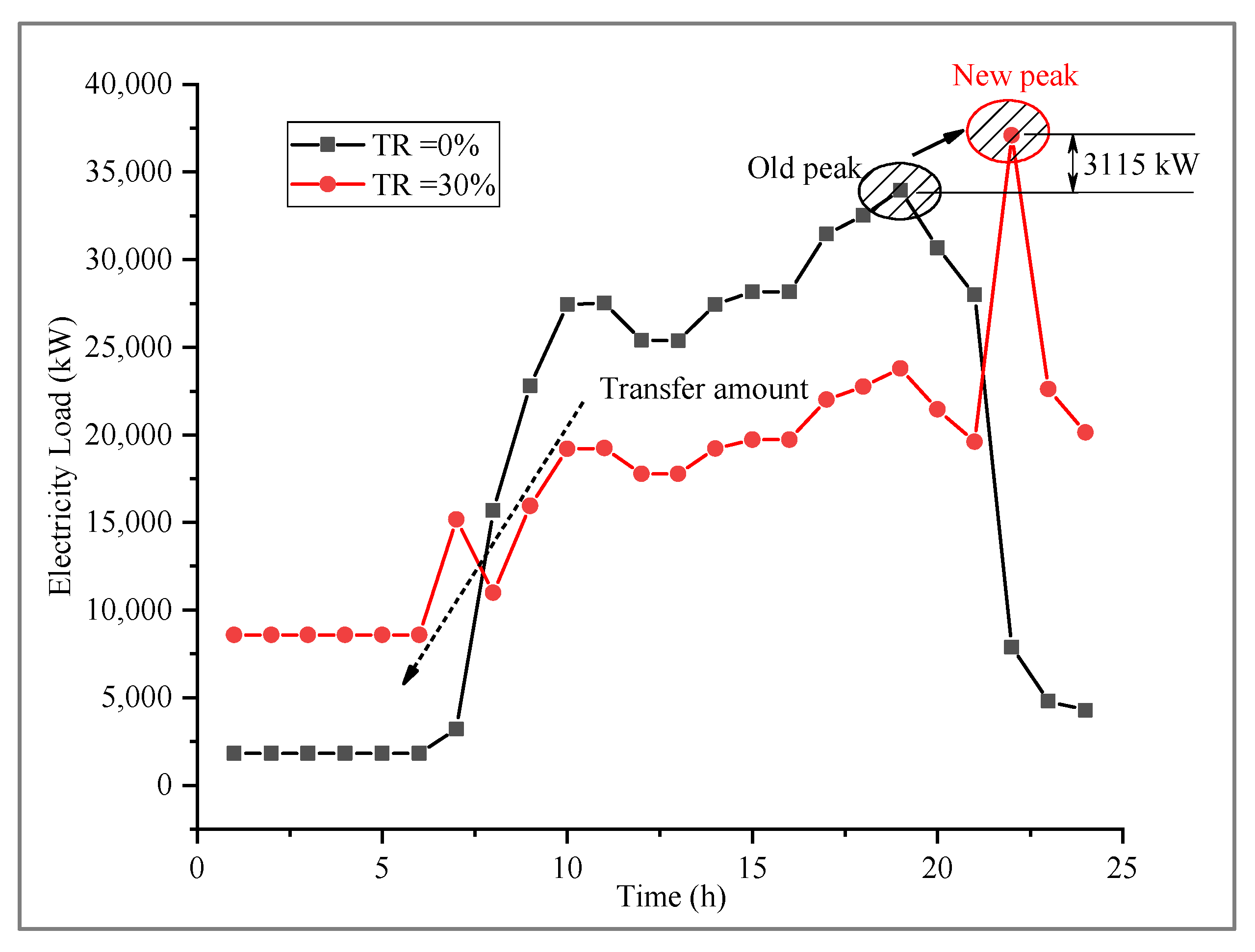
• The amount of peak load transfer represents the energy demand transferred from the peak segment to the valley segment
• The PIES considers cooling storage to produce cooling with the lowest cost
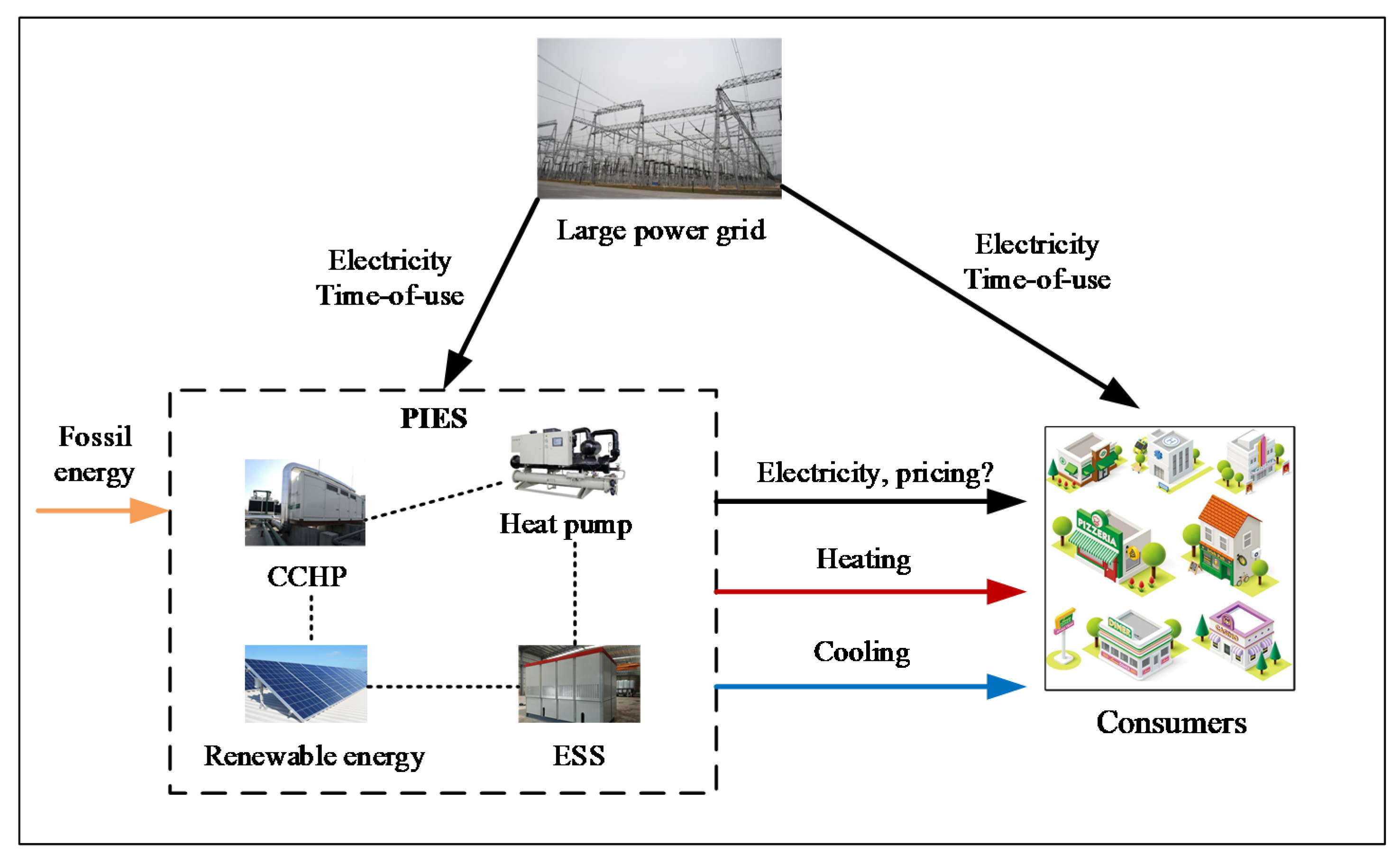
• The cooling and heating required by the consumers originate only from the PIES.

3. P-M Model

The pricing mechanism model (P-M) model consists of two sub-models: the C-P sub-model and the S-P sub-model. The first step in establishing the P-M model is to calculate the cost price of cooling, heating, and electricity in the PIES. On this basis, the S-P sub-model is established considering the profits of PIES and the benefits to consumers, comprehensively. When the energy demand of consumers is fixed (without the demand change caused by DR), the unit energy production cost, which is obtained by calculating the energy configuration of the PIES in the case of the annual minimum cost, is the lowest cost price. Hence, the C-P sub-model of cooling, heating, and electricity can be obtained by the extension of optimal configuration model. The basic modeling principle of the C-P sub-model in this study is to convert the complex modeling and solving process into a computed quantity. In other words, each moment is considered as a basic model unit, and the iterative calculation of the basic model is performed over the entire year.

3.1. C-P Sub-Model

3.1.1. Construction of C-P Sub-Model

The cost price of cooling, heating, and electricity equals the total cost divided by the total energy at time $t$, as shown in Equation (1), where $fva{l}_t^c$, $fva{l}_t^h$, and $fva{l}_t^e$ represent the total costs of cooling, heating, and electricity, respectively. $Q_t^c$ can be obtained by summing the output of all the cooling devices at time $t$, as well as $Q_t^h$ and $Q_t^e$ for the heating and electrical devices, respectively, as shown in Equation (2).

$$P{r}_t^c=\frac{fva{l}_t^c}{Q_t^c},P{r}_t^h=\frac{fva{l}_t^h}{Q_t^h},P{r}_t^e=\frac{fva{l}_t^e}{Q_t^e}$$

(1)

$$Q_t^c={\displaystyle \sum }_i{Q}_{t,i}^c,Q_t^h={\displaystyle \sum }_j{Q}_{t,j}^h,Q_t^e={\displaystyle \sum }_k{Q}_{t,k}^e$$

(2)

Parameter $fva{l}_t^e$ comprises the operating costs, initial investment, and maintenance costs of all power generation equipment, as shown in Equation (3).

$$fva{l}_t^e={\sum }_k(P{r}_{t,k}\ast \frac{Q_{t,k}^e}{{\eta }_k^e}+a\ast I{V}_k\ast \frac{Q_{t,k}^e}{{\sum }_{\tau =1}^{8760}{Q}_{\tau ,k}^e}+M_{t,k}$$

(3)

The large power grid, which supplies electricity to the PIES in the time-of-use mode, is treated as power generation equipment in this study. For the operating costs, $P{r}_{t,k}$ represents the price of fossil energy consumed by each power generation device at time $t$, and $P{r}_{t,k}=0$ represents renewable energy power generation. Meanwhile, ${\eta }_k^e$ represents the efficiency of power generation equipment $k$, which varies with the part load ratio. The initial investment of every device is apportioned at each moment throughout the life cycle according to the time-by-time output, where $a$ is the coefficient of the uniform annual value; $I{V}_k$ is the initial investment of power generation device $k$, which can be calculated by the maximum capacity of device $k$ for the entire year; and ${\sum }_{\mathsf{\tau }=0}^{8760}{Q}_{\tau ,k}^e$ represents the total output of all power generation equipment over the entire year. $M_{t,k}$ represents the maintenance costs, which can be obtained by ref. [23]. Different from the micro-grid, the process of cooling and heating production consumes the internal electricity of park $P{r}_t^e$. $P{r}_t^e$, calculated by Equation (1), is different from the electricity price of the large power grid. In addition, $P{r}_{t,i}$ and $P{r}_{t,j}$ represent the price of fossil energy consumed by each cooling and heating device at time $t$, respectively. Therefore, $fva{l}_t^c$ and $fva{l}_t^h$ are expressed as Equations (4) and (5), where $CO{P}_i^c$ and $CO{P}_j^h$ represent the efficiencies of cooling device $i$ and heating device $j$, respectively, which vary with the part load ratio.

$$fva{l}_t^c={\displaystyle \sum }_i\left(P{r}_{t,i}\ast \frac{Q_{t,i}^c}{{\eta }_i^c}+P{r}_t^e\ast \frac{Q_{t,i}^c}{CO{P}_i^c}+a\ast I{V}_i\ast \frac{Q_{t,i}^c}{{\sum }_{\tau =1}^{8760}{Q}_{\tau ,i}^c}+M_{t,i}\right)$$

(4)

$$fva{l}_t^h={\displaystyle \sum }_j\left(P{r}_{t,j}\ast \frac{Q_{t,j}^h}{{\eta }_j^h}+P{r}_t^e\ast \frac{Q_{t,j}^h}{CO{P}_j^h}+a\ast I{V}_j\ast \frac{Q_{t,j}^h}{{\sum }_{\tau =1}^{8760}{Q}_{\tau ,j}^h}+M_{t,j}\right)$$

(5)

The objective function is the minimum total cost at time $t$, as shown in Equation (6). This is a multivariable constrained nonlinear programming problem that can be solved by FMINCON in Matlab2018b. The constraints include those on supply and demand balance, energy conversion efficiency, equipment, renewable energy, and other nonlinear constraints [23,24], as shown in Equation (7).

$$min(fva{l}_t^e+fva{l}_t^c+fva{l}_t^h)$$

(6)

$$const.\{\begin{array}{c}\mathit{A}·\mathit{Q}\le \mathit{b}\\ {\mathit{A}}_{\mathit{e}\mathit{q}}·\mathit{Q}={\mathit{b}}_{\mathit{e}\mathit{q}}\\ \mathit{l}\mathit{b}\le \mathit{Q}\le \mathit{u}\mathit{b}\\ c\left(\mathit{Q}\right)\le 0\\ c_{eq}\left(\mathit{Q}\right)=0\\ {\mathit{Q}}_{\mathbf{0}}\end{array}$$

(7)

where $\mathit{Q}$ is the column vector of $Q_{\tau ,i/j/k}$; $\mathit{A}·\mathit{Q}\le \mathit{b}$ is the linear inequality constraint, which mainly includes coupling constraints between energy networks, such as the lithium bromide cooling constraint between the micro-cooling network and the micro-grid, and the lithium bromide heating constraint between the micro-heating network and the micro-grid; ${\mathit{A}}_{\mathit{e}\mathit{q}}·\mathit{Q}={\mathit{b}}_{\mathit{e}\mathit{q}}$ is the linear equality constraint, which mainly includes energy conservation constraints; $\mathit{l}\mathit{b}\le \mathit{Q}\le \mathit{u}\mathit{b}$ is the upper and lower limit constraint, which mainly includes the output upper limit constraint of each equipment (natural resource constraint), such as the maximum installed capacity of photovoltaic power generation; $c\left(\mathit{Q}\right)\le 0$ is a nonlinear inequality constraint; $c_{eq}\left(\mathit{Q}\right)=0$ is a nonlinear equality constraint; and ${\mathit{Q}}_{\mathbf{0}}$ is the initial value.

Through solving the optimization model above, the cost prices of cooling, heating, and electricity at time $t$ can be obtained by inputting the power price of the large power grid, the gas price, and the basic parameters of all energy production and conversion equipment.

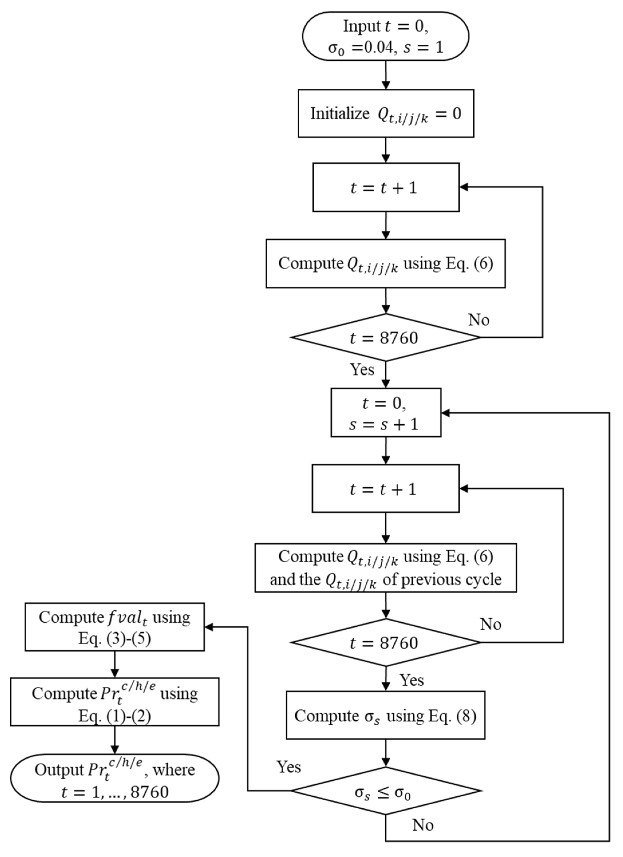
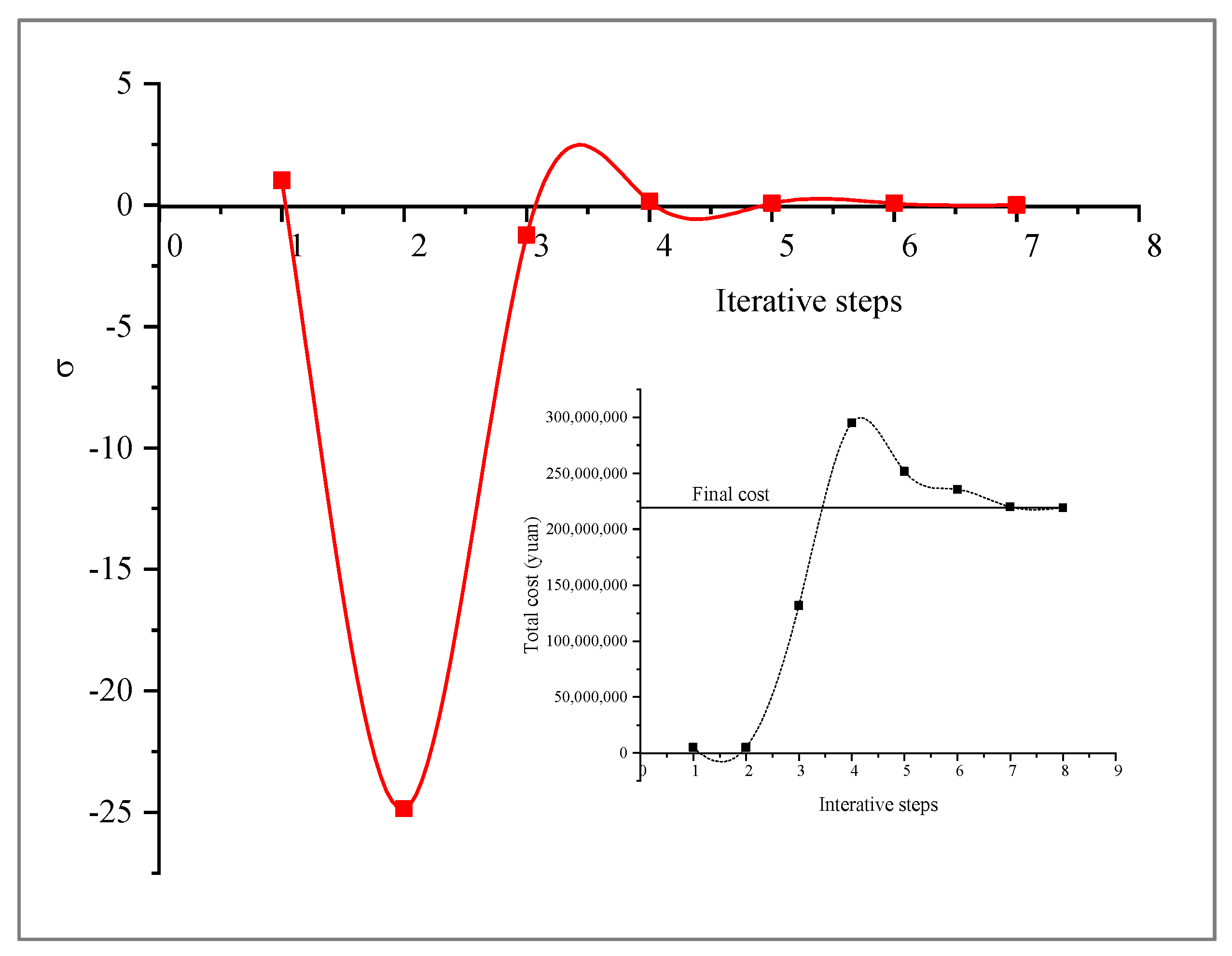
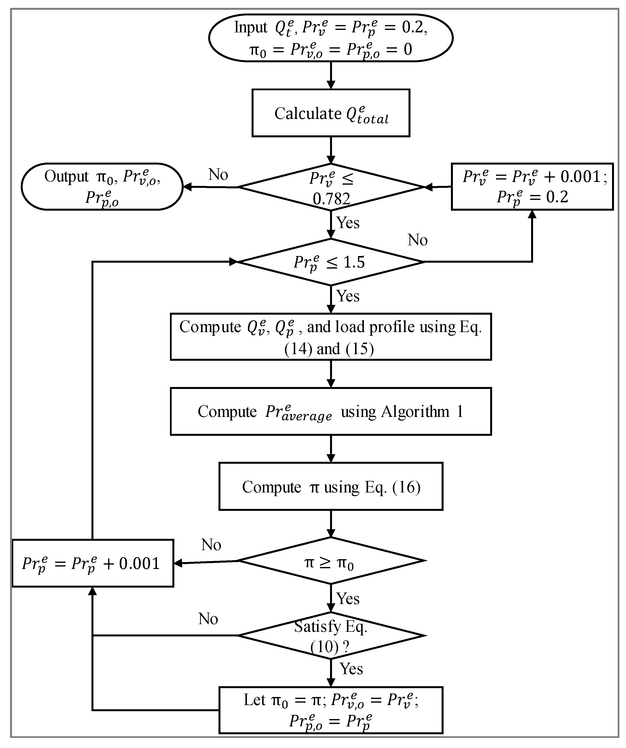
3.1.2. Algorithm of C-P Sub-Model

However, obtaining the energy cost price information at time $t$ only is not sufficient. It is necessary to calculate the hourly energy cost price of the PIES through a loop iteration over the entire year. In addition, the control index of the loop iteration is expressed in Equation (8), where $s$ represents the number of iteration steps, and $fva{l}_{total}^s$ represents the total cost during the entire year.

$${\mathsf{\sigma }}_s=\frac{fva{l}_{total}^s-fva{l}_{total}^{s-1}}{fva{l}_{total}^{s-1}}$$

(8)

On this basis, Algorithm (1) can be used to perform the loop iteration of the C-P sub-model over the entire year, as illustrated in Figure 2. For starting time $t=1$, $max\left(Q_{t,i/j/k}\right)={\sum }_{\tau =1}^{8760}\left|Q_{\tau ,i/j/k}\right|=Q_{t,i/j/k}$, and Equation (6) is called to calculate $Q_{1,i/j/k}$. When $t=2$, $max\left(Q_{t,i/j/k}\right)=Q_{1,i/j/k} or Q_{2,i/j/k}$, ${\sum }_0^{8760}\left|Q_{\tau ,i/j/k}\right|=Q_{1,i/j/k}+Q_{2,i/j/k}$, and Equation (6) is called to calculate $Q_{2,i/j/k}$. Similarly, when $t=t+1$, $Q_{t+1,i/j/k}$ can be calculated until $t=8760$. When the second loop starts, namely $t=1$ again, Equation (8) is the determinator of iterative convergence. The iterative process continues until ${\mathsf{\sigma }}_s\le 0.04$.

The C-P sub-model and loop iterative method are applied in practical engineering, and the annual hourly cost price of PIES is captured under different load profiles, which provides support for the construction of the S-P sub-model.

3.2. S-P Sub-Model

3.2.1. Construction of S-P Sub-Model

How is the selling price used to trade with consumers determined from the hourly cost price of cooling, heating, and electricity? The easiest method is to set the energy selling price as a constant over the entire year. Then, the selling price can be calculated by a given annual profit rate and obtained cost price. The annual profit rate of the PIES, $p^{\prime }$, can be calculated by Equation (9) [25].

$$p^{\prime }=\frac{{\sum }_{t=1}^{8760}(Q_t^e(P{r}^e-P{r}_t^e)+Q_t^c\left(P{r}^c-P{r}_t^c\right)+Q_t^h\left(P{r}^h-P{r}_t^h\right))}{{\sum }_{t=1}^{8760}\left(fva{l}_t^e+fva{l}_t^c+fva{l}_t^h\right)}$$

(9)

where $P{r}^e$, $P{r}^c$, and $P{r}^h$ represent the selling prices of electricity, cooling, and heating, respectively. Under the assumption mentioned above, when the selling prices of cooling, heating, and electricity vary independently, the linear relationship of annual profit rate with energy selling price can be obtained by using Equation (9). Furthermore, $P{r}^e$, $P{r}^c$, and $P{r}^h$ are determined by black calculation.

From the perspective of cooling and heating, owing to the large delay in the supply and delivery of cooling and heating [26], it is meaningless to adjust the selling price of cooling and heating on an hourly basis. Therefore, in this study, the same cooling or heating selling price throughout the year is adopted. From the perspective of electricity, the pricing mode with the same electricity price through the entire year will increase the polarization of the load. This is because compared with the time-of-use pricing mode of the large power grid, the lower-priced electricity supplied by the PIES during the hours of peak demand leads to higher electricity consumption, and the higher-priced electricity during the hours of valley demand leads to less electricity consumption. Evidently, the static pricing mode is very inappropriate for the PIES. The time-of-use pricing mode and real-time pricing mode, which are advantageous for load leveling, should be adopted.

For consumers, there are two electricity suppliers: the large power grid and the PIES, as shown in Figure 1. The consumers, having no generation capability, need to purchase all their required energy from the PIES or the large power grid or other suppliers. However, there are no municipal heating networks and other cooling suppliers in the hot summer and cold winter zones in China. Hence, the consumers can only obtain cooling and heating from the PIES. From the perspective of economic efficiency, the consumers will choose the lowest electricity supplier. This study assumes that a consumer cannot select two electricity suppliers simultaneously and can switch, at most, once a day. Hence, the constraint when consumers select PIES as the electricity supplier is shown in Equation (10), where $Q_t^e$ is the amount of electricity from the PIES consumed by the consumers at time $t$; $P{r}_t^{e,s}$ is the selling price of electricity at time $t$; $Q_t^{pg}$ is the amount of electricity from the large power grid consumed by the consumers at time $t$; and $P{r}_t^{pg}$ is the time-of-use electricity price of the large power grid.

$${\displaystyle \sum }_{t=1}^{24}(Q_t^{e}P{r}_t^{e,s})\le {\displaystyle \sum }_{t=1}^{24}(Q_t^{pg}P{r}_t^{pg})$$

(10)

In general, the buying price set by the large power grid is considerably lower than its selling price without subsides [27]. Hence, the feed-in tariff scheme of the PIES is unreasonable when the renewable energy penetration is not high. In addition, when the electrical load reaches its peak, the electricity cost price also reaches its peak. From an economical perspective, $P{r}_t^{e,s}$ needs to be formulated for the following reasons: (1) decrease the electricity consumption at the peak; (2) increase the electricity consumption at the valley; (3) promote the profitability of the PIES; and (4) reduce the electricity bill of the consumers. In this study, the total daily electricity consumption of PIES is kept unchanged after $P{r}_t^{e,s}$ is formulated [28]. The reduction in the electricity bill of consumers is used as the constraint, as shown in Equation (10). Hence, the objective function is the maximum benefit for the PIES, as shown in Equation (11), where $P{r}_t^e$ represents the cost price of electricity at time $t$.

$$\pi =max[{\displaystyle \sum }_{t=1}^{24}(Q_t^e\left(P{r}_t^{e,s}-P{r}_t^e\right))]$$

(11)

In Equation (11), as $P{r}_t^{e,s}$ increases during the peak demand phase, and $P{r}_t^{e,s}$ decreases during the valley demand phase, the load curve of consumers tends to level according to the Cross-Price Elasticity of Demand theory [29]. Hence, the functional relationship between the demand and price at each moment is presented in Equation (12). Equation (12) is subjected to Equation (13), where $Q_{total}^e$ represents the total daily electricity demand.

$$Q_t^e=f\left(P{r}_1^{e,s}, P{r}_2^{e,s},\dots ,P{r}_{24}^{e,s}\right)$$

(12)

$$Q_{total}^e={\displaystyle \sum }_{t=1}^{24}(Q_t^e)$$

(13)

Substituting Equation (12) into Equation (11) yields $\pi =max\left[g\left(P{r}_1^{e,s}, P{r}_2^{e,s},\dots ,P{r}_{24}^{e,s}\right)\right]$, because $P{r}_t^e$ is a function of $Q_t^e$ according to the C-P sub-model in Section 3.1.1. In summary, $\pi$ represents the maximum benefit to the PIES considering the comprehensive effects of demand and configuration changing in the planning and design stages.

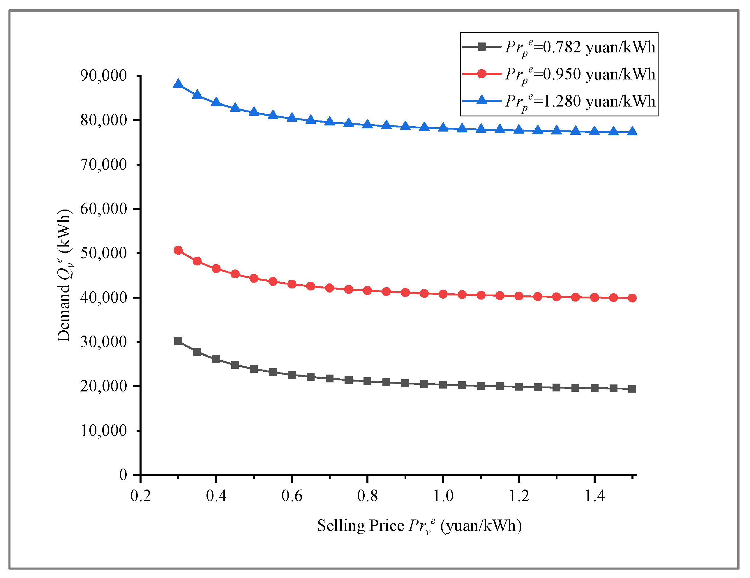
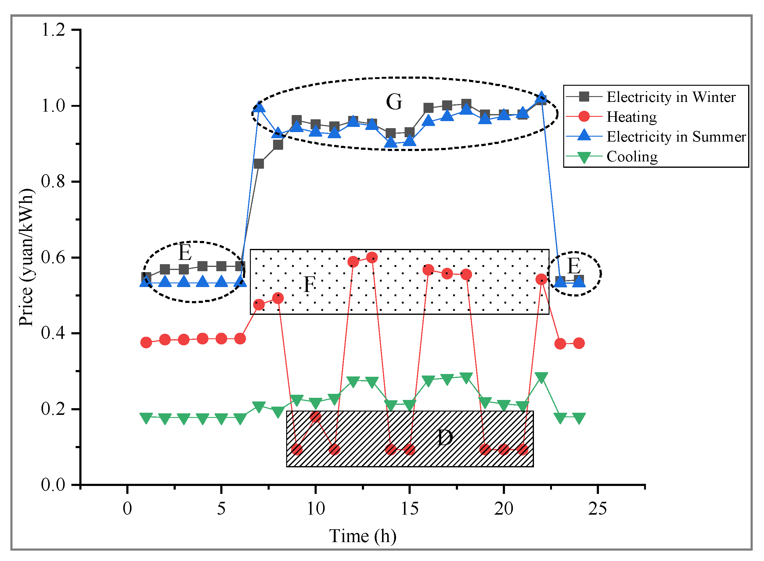
3.2.2. Price Pattern and Demand Function

The energy market composed of PIES, the large power grid, and consumers can be described by a typical Price Leadership Model [30]. However, as the time-of-use electricity price of the large power grid does not change with the energy transaction in the actual PIES project, Equation (11) can describe the market behavior under this mode fully, instead of the Price Leadership Model.

In actual engineering, Equation (12) is difficult to calculate because the real-time electricity price changes hourly. Additionally, the existing literature shows that the participation of consumers in real-time electricity price is very low [31]. Hence, it is impractical to implement real-time electricity pricing in the PIES. The time-of-use electricity price uses a static price scheme based on a predefined selling price, which usually maintains the same daily electricity price throughout the week, the month, the season, or the entire year [32]. The advantages of time-of-use pricing scheme include the following: (1) it is easy to follow; (2) it has a stable daily participating ratio; and (3) it can effectively shift the peak loads to valley loads [33]. Additionally, from Section 2, as the load and electricity cost price are divided into a peak segment and valley segment, a two-stage time-of-use electricity price is adopted to determine the electricity selling price of the PIES. The reasons for adopting the two-stage time-of-use electricity price will be also described in Section 4.1. Ref. [34] provides the cross-price function of the demand, as shown in Equation (14). Meanwhile, instead of Equation (12), Equation (14) is substituted into Equation (11).

$$\{\begin{array}{c}{Q}_v^e=\alpha +{\beta }_v{\left(P{r}_v^e\right)}^{\gamma }+{\beta }_{p}P{r}_p^e\\ 0.2\le P{r}_v^e\le 0.782\\ 0.2\le P{r}_p^e\le 1.5\end{array}$$

(14)

where $Q_v^e$ is the valley electricity consumption; $P{r}_v^e$ represents the valley selling price; $P{r}_p^e$ represents the peak selling price; and $\alpha$, ${\beta }_v$, $\gamma$, and ${\beta }_p$ are the preference parameters [35]. In Equation (14), the demand function is derived by seeking the extremum of the utility function [14]. The relationships between $Q_v^e$ and $P{r}_v^e$ ($P{r}_p^e$) are illustrated in Figure 3. From Equation (14) and Figure 3, $Q_v^e$ is proportional to $P{r}_p^e$ and decreases as $P{r}_v^e$ increases. According to Equation (13), the electricity consumption at peak $Q_p^e$ can be calculated as follows:

$$Q_p^e=Q_{total}^e-Q_v^e.$$

(15)

On this basis, Equation (11) is transformed into Equation (16).

$$\pi =max\left[Q_v^{e}P{r}_v^e+Q_p^{e}P{r}_p^e-Q_{total}^{e}P{r}_{average}^e\right]$$

(16)

where $P{r}_{average}^e$ represents the average electricity cost price, which can be calculated by C-P sub-model. In general, $P{r}_{average}^e$ is a variable that changes as the configuration capacity and TR change. The TR is the ratio of the shifted load to the total peak load, which can be calculated by Equation (17), where $Q_p^e{}^{\prime }$ is the total peak electricity consumption in peak before the load shift.

$$TR=\frac{Q_p^e{}^{\prime }-Q_p^e}{Q_p^e{}^{\prime }}$$

(17)

At this point, the S-P sub-model is completed.

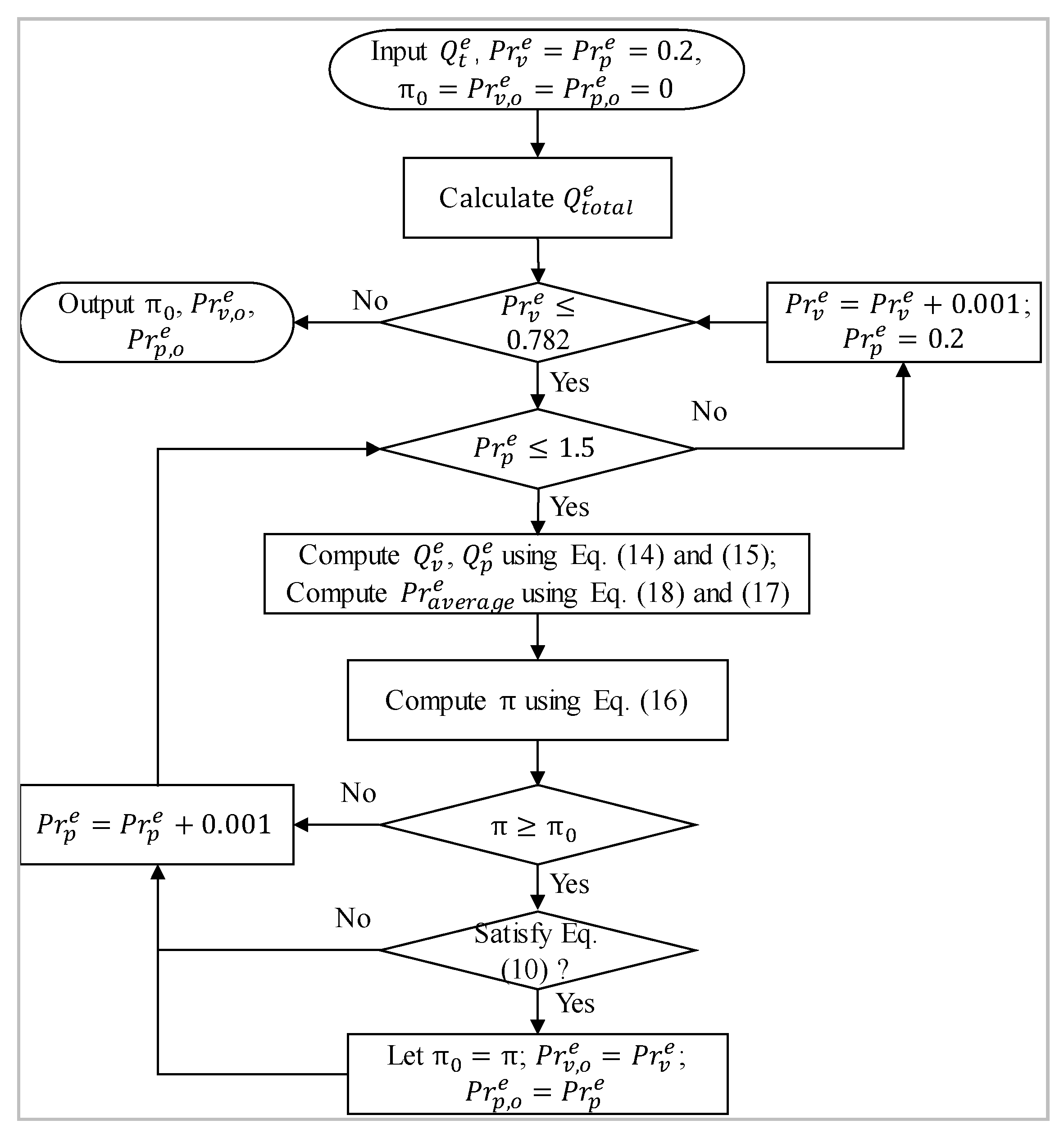
3.2.3. Algorithm of S-P Sub-Model

The types of energy that the PIES trades with consumers include cooling, heating, and electricity. The selling prices of cooling and heating can be obtained by Equation (9). Hence, this section focuses on solving and discussing the optimized results of the electricity price in the P-M model. Algorithm 2 can be used to solve the P-M model, and the flowchart of Algorithm 2 is shown in Figure 4. In Figure 4, $P{r}_{v,0}^e$ and $P{r}_{p,0}^e$ represent the valley electricity selling price and peak electricity selling price, respectively when $\pi$ is maximum.

In summary, the selling price of cooling, heating, and electricity in the PIES can be formulated by solving the P-M model composed of the C-P sub-model and the S-P sub-model, considering the comprehensive effects of demand and configuration changing in the planning and design stages. In the following, a numerical study of the above P-M model is presented.

4. Numerical Study

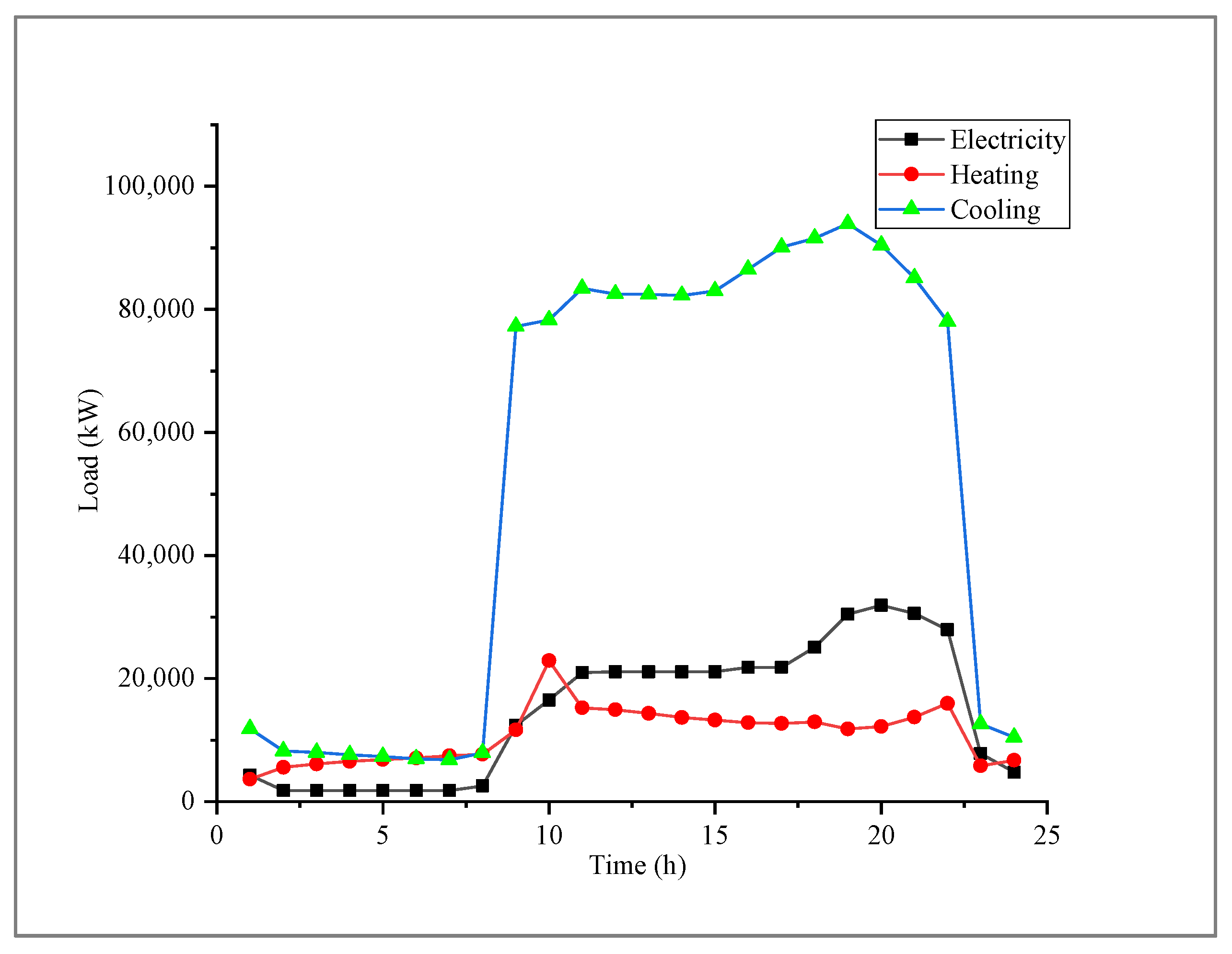
4.1. Essential Information and Preliminary Calculation

In this study, a real PIES located in Shanghai, China, has been selected as a case study to verify the P-M model developed in this study. The energy production equipment of PIES mainly includes absorption refrigeration units, gas generators, photovoltaics, photothermal, heat pumps, boilers, chillers, energy storage equipment, wind power, and so on. The total area of energy supplying is 960,000 square meters, including an office building area of 479,000 square meters, commercial building area of 383,000 square meters, and hotel building area of 98,000 square meters. The hourly load of cooling, heating, and electricity in the typical day are illustrated in Figure 5. Meanwhile, there is no effect of DR, i.e., TR = 0. In addition, owing to the delayed effect of cooling and heating transport, achieving the DR of cooling and heating is very difficult. Hence, the TR only refers to the electrical shifted load caused by the DR.

The annual hourly load, the basic data, and the constraints of the above-mentioned energy production equipment are input into the C-P sub-model. Then, the loop iterative method (Algorithm (1)) is applied in the case, and the annual hourly cost price of PIES is captured, which are shown in Figure 6. The curve of ${\mathsf{\sigma }}_s$ varies with the iteration steps in the solution process, as shown in Figure 7, which illustrates that the iteration process converges quickly. From Figure 7, the total cost of the PIES first increases; then, it decreases, and it finally stabilizes at the final cost. Figure 6 shows that the average cost price of cooling is the lowest, and the fluctuation in the cost price is smoothest. The fluctuation in the electricity cost price in winter and summer are similar, and the former is slightly higher than the latter. The heating cost price in zone D is lower than the price at other times during the winter heating period. The reason is that the CHP is chosen to supply electricity to the PIES because the electricity price of the large power grid is at a peak in zone D and can provide free heating through the additional waste heat. The heating cost price of zone F is higher because of the gas boiler. Since the cost price of zone G and zone E differs greatly in the electricity cost price curve, the daily electricity cost price is divided into a peak segment (G) and a valley segment (E) in the following studies, as shown in Section 2.

When the DR occurs, i.e., TR ≠ 0, the cost price of cooling, heating, and electricity should be recalculated by using the C-P sub-model and Algorithm (1) according to the load profile at this time. The TR and new load peaks under 12 scenarios of load profiles are illustrated in

Table 1. Twelve different scenarios of load profiles due to load shift.

Number	1	2	3	4	5	6
TR/%	−5	0	5	10	12.5	15
Maximum load/kW	35,673	33,974	32,275	30,577	29,727	28,878
Number	7	8	9	10	11	12
TR/%	17.5	20	21.5	25	27.5	30
Maximum load/kW	28,028	27,353	28,813	32,221	34,655	37,089

.

The average daily electricity cost prices ($P{r}_{average}^e$) are illustrated in Figure 6 under the 12 different load profiles. As shown in Figure 8, the configuration ratio is the ratio of the maximum installed capacity at a certain TR to the maximum installed capacity at TR = 0. Some interesting rules have been discovered by processing the solution results of the 12 different load profiles, as follows. First, from the perspective of the initial investment, as the TR increases, the configuration ratio drops from point B to point A and then rises to point C. At point A, the PIES has the smallest installed capacity. The installed capacity at point C is higher than the installed capacity before the load shifted, which means that the excessive load shift generates a new peak in electrical demand, as shown in Figure 9. From Figure 9, when TR = 30%, the peak load is shifted to 22:00 from 19:00, and the new peak is 3115 kW larger than the old peak. The emergence of the new peak means that the load shift does not reduce the initial investment. Therefore, in Figure 8, the load shift scenario above the black dotted line (original configuration line) does not produce a positive effect for the initial investment reduction. Second, from the perspective of operating costs, on the one hand, with the reduction in the PIES installed capacity, the energy conversion efficiency increases for a partial load. Therefore, the cost price of electricity decreases at this time. On the other hand, the load shift transfers the electricity from the peak electricity price period of the large power grid to the valley electricity price period. This means that the valley electricity consumption increases as TR increases, which causes a reduction in the daily average cost of electricity in the PIES. Comprehensively considering initial investments and operating costs, the average cost price drops rapidly before point A’, and then the falling speed is reduced after point A’, as shown in Figure 8. The changing process in the average electricity cost price $P{r}_{average}^e$ can be fitted to Equation (18), where $TR$ is the ratio of the shifted load from G zone to E zone (Figure 6) to the total peak load. In particular, the necessary condition of Equation (18) is that the PIES is rationally configured under different load profiles. In fact, in the solution process, the C-P sub-model, which is a sub-module of the P-M model, should be re-optimized in each call. Algorithm (3) can be used to solve the P-M model, and the flowchart of Algorithm (3) is shown in Figure 10. However, because the C-P sub-model involves a large amount of calculation and long calculation time, a regression equation is used to simplify the solution process. This is to say, Equation (18) is substituted into Equation (16).

$$P{r}_{average}^e=5.57T{R}^3-3.098T{R}^2-0.1133TR+0.8633R^2=0.991$$

(18)

The average daily cost prices of cooling and heating are shown in Figure 11. The shift in demand of cooling and heating is ignored in this study, and TR refers to the proportion of power demand shift illustrated in Figure 11. It can be seen from Figure 11 that as the TR increases, the change in the average cooling cost price is just miniscule, but the heating cost price gradually increases. The increase in the heating cost price is caused by the following progressive relationship: (1) a load shift causes the increase in valley electricity consumption; (2) consequently, the installed capacity and operating hours of CHP (combined heating and power) are reduced; (3) this leads to a reduction in the free heating provided by the CHP; (4) eventually, the heating cost price increases. Since the proportion of free cooling provided by the CHP to the total cooling is low, the change in the cooling cost price is small. However, the maximum increase in the heating cost price is only 0.04 yuan/kWh. Therefore, the changes in the cooling and heating cost price caused by the electricity DR are ignored in this study.

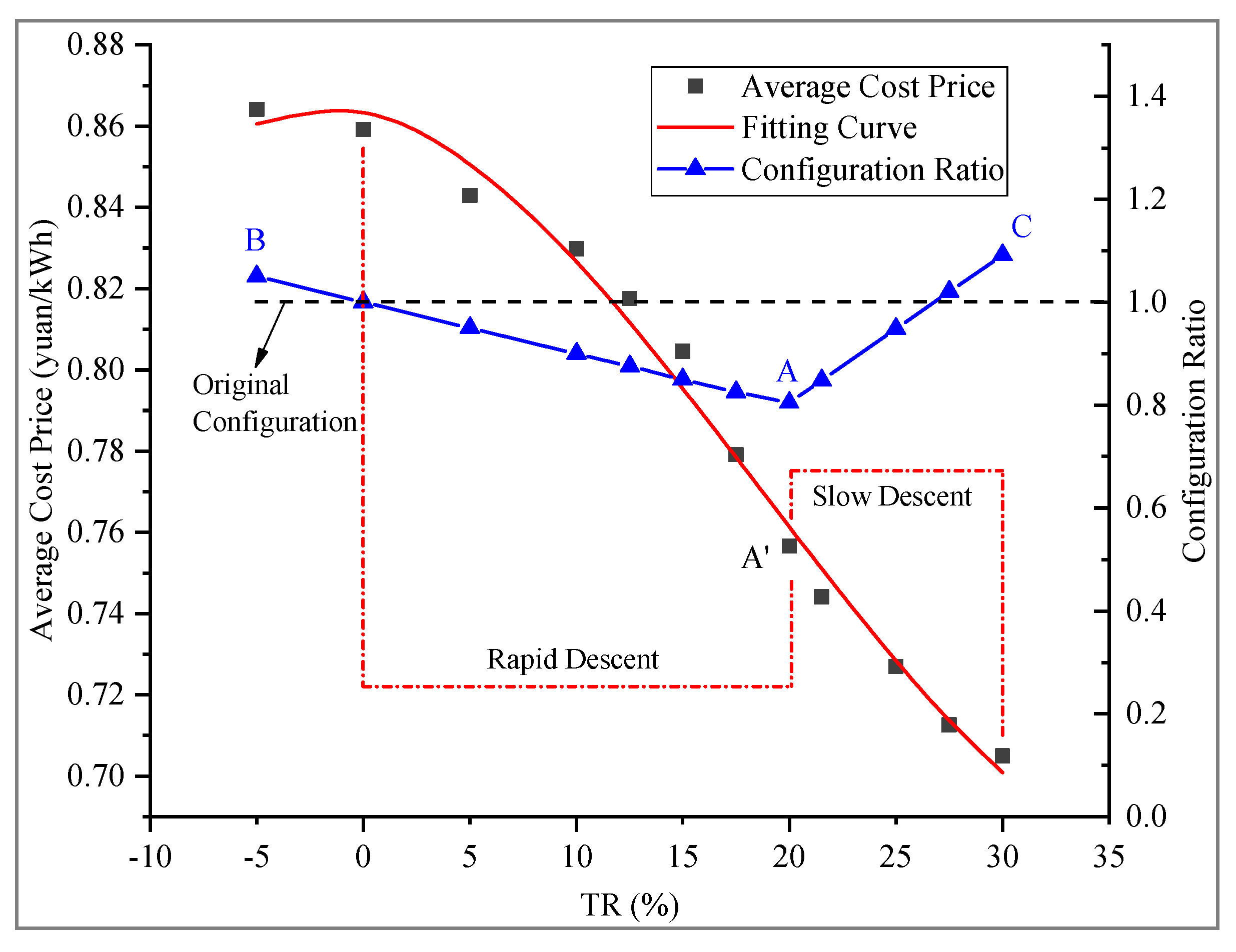
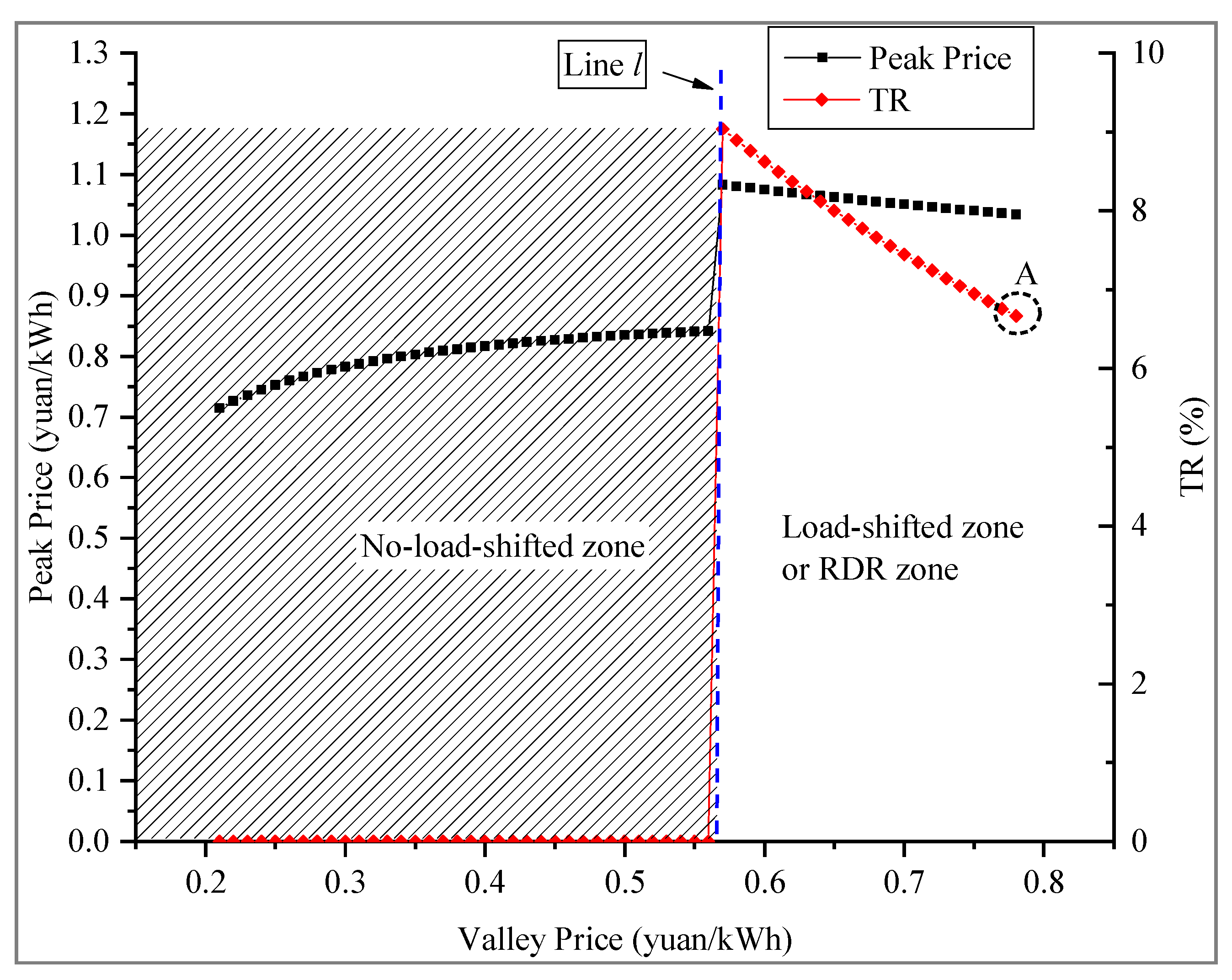
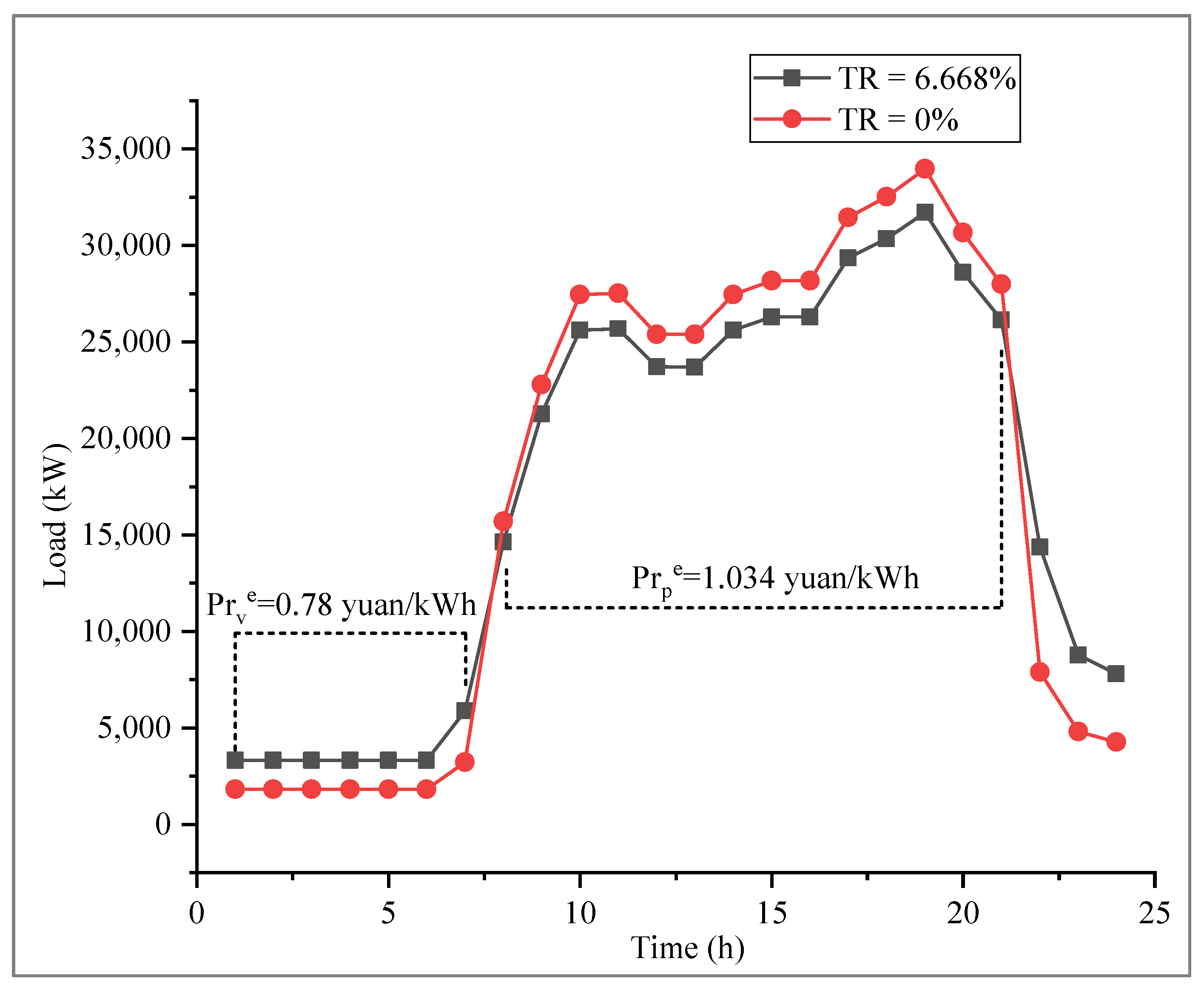
4.2. Results and Discussion

Using Algorithm (2), the following results can be calculated under a series of valley electricity selling prices $P{r}_v^e$: (1) the maximum profit of PIES; (2) the optimal peak electricity selling price; (3) the maximum profit of consumers; and (4) the optimal TR. In Figure 11, the left area of the dotted line l is the benefit-sharing zone, which means that the total profit generated by changing the peak and valley electricity selling price is shared by consumers and PIES. In the benefit-sharing zone, as the valley electricity selling price increases, the peak electricity selling price increases gradually in order to make the PIES gain the maximum profit, while the consumers profits decrease slowly. Additionally, from Figure 12, the total profit is constant in the benefit-sharing zone. The reason is that the left area of the dotted line l has no load shifted, as shown in Figure 13. In the benefit-sharing zone of Figure 12, point B is the optimal solution of the P-M model; that is, the daily profit of PIES is 337,861 yuan, the peak selling price is 0.842 yuan/kWh, the valley selling price is 0.56 yuan/kWh, and the consumers’ electricity bill reduction is 63,421 yuan. In order to reflect the effectiveness of the proposed pricing model, the economic benefits are calculated without considering the impact of demand shift on the capacity of the PIES in the planning and design stage, based on the existing typical price leadership model. The results show that using the proposed model can reduce the initial investment of PIES by 10.69 million yuan and increase the total daily profit by 21,967 yuan, including PIES and consumers. Furthermore, from Figure 12, the right area of the dotted line l is the benefit-exclusive zone, which means that the total profit is taken by the PIES, and the consumers do not need to pay extra for the electricity compared with that associated with using the large power grid. The benefit-exclusive zone in Figure 12 corresponds to the load-shifted zone in Figure 13. In the benefit-exclusive zone, in order to reduce electricity bills, the consumers will adjust their energy habits (by DR) according to the time-of-use scheme formulated by the PIES. In fact, this adjustment (by DR) will neither reduce electricity bills nor increase electricity bills, as shown in Figure 12. Therefore, the adjustment of consumers in the benefit exclusive zone is meaningless for consumers, which is called the reactive demand response (RDR) in this paper. However, for the PIES, the RDR brings some profit growth, as shown in Figure 12. From the perspective of the total benefit for consumers and the PIES, the total profit in the RDR zone is lower than the total profit in the the benefit-sharing zone. In addition, if the valley price resides in the RDR zone for a long time, the consumers will find this trap based on actual experience and, thus, refuse to respond to the time-of-use scheme of PIES. Hence, the TR will drop to zero; that is, it will return to the no-load-shifted zone (benefit sharing zone), as shown in Figure 13. In summary, from the perspective of the long-term benefit, the PIES sharing its profits with consumers (the benefit sharing zone) is the ultimate choice for PIES and consumers; that is, point B is the optimal solution for the long-term situation.

Additionally, from the perspective of P-M model optimization, point A in Figure 12 can be considered as the optimal solution for the short-term scenario. At point A, it is possible to ensure a reduction in the peak load and an increase in the valley load, simultaneously, corresponding to a PIES daily profit of 357,725 yuan, a peak selling price of 1.034 yuan/kWh, a valley selling price of 0.78 yuan/kWh, and a TR of 6.668%. The shifted load of point A is illustrated in Figure 14, where no new peak appears.

5. Conclusions

With the opening of the Chinese electricity market, the park-integrated energy system (PIES) appeared as an energy service provider. Under this new energy market mode, some new problems need to be addressed urgently: (1) How could we formulate the energy selling price so that the consumers spend less money and the PIES obtains more benefits? (2) How could we quantify the effects of DR on the PIES configuration? (3) How could we quantify the impact of the installed capacity on the energy selling prices? To resolve these problems, a P-M model was proposed in the planning and design stages of the PIES. The P-M model consisted of two sub-models: the C-P sub-model and the S-P sub-model. In the C-P sub-model, DR and energy configuration (types, capacities, and strategies of equipment) were both considered. Using the C-P sub-model, the cost price of cooling, heating, and electricity were obtained under 12 different load profiles. Then, the function relationship between the energy cost price and TR was established through regression analysis. In the S-P sub-model, two pricing schemes were given. One is that prices remain constant throughout the entire year, which is suitable for cooling and heating. The other is the two-stage time-of-use pricing scheme, which is suitable for electricity. The hourly electrical price was obtained by using the S-P sub-model, which was beneficial to both PIES and consumers.

In numerical studies, an RDR zone was found, where the DR of consumers did not bring a reduction in the electricity bill, and from the perspective of the long-term benefit, the DR of consumers would disappear. The results indicate that the PIES sharing its profits with consumers (in the benefit-sharing zone) is the ultimate choice for PIES and consumers; that is, point B is the optimal solution for the long-term situation. From the perspective of P-M model optimization, it can be considered that point A is the optimal solution for the short-term scenario. This study can provide the owners of PIES with a suggestion that win–win is the optimal choice in energy pricing and a method for determining the optimal energy selling price. Furthermore, it would be compelling to focus on the free competitive energy market involving multiple PIESs in future research. However, the biggest obstacle of model application in the real world is that when the user group reaches a certain size and the information flow is unobstructed between users, the users will only respond to the benefits exceeding a certain value. In addition, the limitations in practical applications also include the accurate prediction of demand load and accurate quantification of demand response. However, these are not the focus of this study. The paper only provides a pricing tool of cooling, heating, and electricity in PIES based on the existing load forecasting and demand response research.

References

1. Roldán-Blay, C.; Escrivá-Escrivá, G.; Roldán-Porta, C. Improving the benefits of demand response participation in facilities with distributed energy resources. Energy 2019, 169, 710–718. [Google Scholar] [CrossRef]
2. Reihani, E.; Motalleb, M.; Ghorbani, R.; Saad Saoud, L. Load peak shaving and power smoothing of a distribution grid with high renewable energy penetration. Renew. Energy 2016, 86, 1372–1379. [Google Scholar] [CrossRef] [Green Version]
3. Shirazi, E.; Jadid, S. Cost reduction and peak shaving through domestic load shifting and DERs. Energy 2017, 124, 146–159. [Google Scholar] [CrossRef]
4. Uddin, M.; Romlie, M.F.; Abdullah, M.F.; Abd Halim, S.; Abu Bakar, A.H.; Chia Kwang, T. A review on peak load shaving strategies. Renew. Sustain. Energy Rev. 2018, 82, 3323–3332. [Google Scholar] [CrossRef]
5. Teo, K.T.K.; Hui Hwang, G.; Bih Lii, C.; Sook Kwan, T.; Min Keng, T. Modelling and optimisation of stand alone power generation at rural area. In Proceedings of the 2013 IEEE International Conference on Consumer Electronics-China, Shenzhen, China, 11–13 April 2013; pp. 51–56. [Google Scholar]
6. Locatelli, G.; Palerma, E.; Mancini, M. Assessing the economics of large Energy Storage Plants with an optimisation methodology. Energy 2015, 83, 15–28. [Google Scholar] [CrossRef] [Green Version]
7. Oudalov, A.; Cherkaoui, R.; Beguin, A. Sizing and Optimal Operation of Battery Energy Storage System for Peak Shaving Application. In Proceedings of the 2007 IEEE Lausanne Power Tech, Lausanne, Switzerland, 1–5 July 2007; pp. 621–625. [Google Scholar]
8. Telaretti, E.; Dusonchet, L. Battery storage systems for peak load shaving applications: Part 2: Economic feasibility and sensitivity analysis. In Proceedings of the 2016 IEEE 16th International Conference on Environment and Electrical Engineering (EEEIC), Florence, Italy, 7–10 June 2016; pp. 1–6. [Google Scholar]
9. Asgharian, H.; Baniasadi, E. Experimental and numerical analyses of a cooling energy storage system using spherical capsules. Appl. Therm. Eng. 2019, 149, 909–923. [Google Scholar] [CrossRef]
10. Mortaz, E.; Valenzuela, J. Optimizing the size of a V2G parking deck in a microgrid. Int. J. Electr. Power Energy Syst. 2018, 97, 28–39. [Google Scholar] [CrossRef]
11. Siano, P. Demand response and smart grids-A survey. Renew. Sustain. Energy Rev. 2014, 30, 461–478. [Google Scholar] [CrossRef]
12. Li, B.; Roche, R.; Paire, D.; Miraoui, A. A price decision approach for multiple multi-energy-supply microgrids considering demand response. Energy 2019, 167, 117–135. [Google Scholar] [CrossRef]
13. Tushar, W.; Chai, B.; Yuen, C.; Smith, D.B.; Wood, K.L.; Yang, Z.; Poor, H.V. Three-Party Energy Management With Distributed Energy Resources in Smart Grid. IEEE Trans. Ind. Electron. 2015, 62, 2487–2498. [Google Scholar] [CrossRef] [Green Version]
14. Pavlidou, F.; Koltsidas, G. Game theory for routing modeling in communication networks-A survey. J. Commun. Netw. 2008, 10, 268–286. [Google Scholar] [CrossRef]
15. Nguyen, D.T.; Nguyen, H.T.; Le, L.B. Dynamic Pricing Design for Demand Response Integration in Power Distribution Networks. IEEE Trans. Power Syst. 2016, 31, 3457–3472. [Google Scholar] [CrossRef]
16. Golmohamadi, H.; Keypour, R.; Bak-Jensen, B.; Radhakrishna Pillai, J. Optimization of household energy consumption towards day-ahead retail electricity price in home energy management systems. Sustain. Cities Soc. 2019, 47, 101468. [Google Scholar] [CrossRef]
17. Wang, D.; Hu, Q.E.; Jia, H.; Hou, K.; Du, W.; Chen, N.; Wang, X.; Fan, M. Integrated demand response in district electricity-heating network considering double auction retail energy market based on demand-side energy stations. Appl. Energy 2019, 248, 656–678. [Google Scholar] [CrossRef]
18. Wang, J.; Yang, W.; Du, P.; Niu, T. Outlier-robust hybrid electricity price forecasting model for electricity market management. J. Clean. Prod. 2020, 249, 119318. [Google Scholar] [CrossRef]
19. Zhang, J.; Tan, Z.; Wei, Y. An adaptive hybrid model for short term electricity price forecasting. Appl. Energy 2020, 258, 114087. [Google Scholar] [CrossRef]
20. Bruno Bernal, J.C.M.; de Gracia, F.P. Impact of fossil fuel prices on electricity prices in Mexico. J. Econ. Stud. 2019, 46, 356–371. [Google Scholar]
21. Peng, X.; Tao, X. Cooperative game of electricity retailers in China’s spot electricity market. Energy 2018, 145, 152–170. [Google Scholar] [CrossRef]
22. Ma, T.; Wu, J.; Hao, L.; Lee, W.-J.; Yan, H.; Li, D. The optimal structure planning and energy management strategies of smart multi energy systems. Energy 2018, 160, 122–141. [Google Scholar] [CrossRef]
23. Guo, L.; Liu, W.; Cai, J.; Hong, B.; Wang, C. A two-stage optimal planning and design method for combined cooling, heat and power microgrid system. Energy Convers. Manag. 2013, 74, 433–445. [Google Scholar] [CrossRef]
24. Liu, Z.; Yu, H.; Liu, R. A novel energy supply and demand matching model in park integrated energy system. Energy 2019, 176, 1007–1019. [Google Scholar] [CrossRef]
25. Lee, J.; Kim, D.R.; Lee, K.-S. Optimum hub height of a wind turbine for maximizing annual net profit. Energy Convers. Manag. 2015, 100, 90–96. [Google Scholar] [CrossRef]
26. Kicsiny, R. New delay differential equation models for heating systems with pipes. Int. J. Heat Mass Transf. 2014, 79, 807–815. [Google Scholar] [CrossRef]
27. McKenna, E.; Thomson, M. Photovoltaic metering configurations, feed-in tariffs and the variable effective electricity prices that result. IET Renew. Power Gener. 2013, 7, 235–245. [Google Scholar] [CrossRef] [Green Version]
28. Srivastava, A.; Van Passel, S.; Laes, E. Assessing the success of electricity demand response programs: A meta-analysis. Energy Res. Soc. Sci. 2018, 40, 110–117. [Google Scholar] [CrossRef]
29. Frondel, M. Empirical assessment of energy-price policies: The case for cross-price elasticities. Energy Policy 2004, 32, 989–1000. [Google Scholar] [CrossRef]
30. Dijkstra, P.T. Price leadership and unequal market sharing: Collusion in experimental markets. Int. J. Ind. Organ. 2015, 43, 80–97. [Google Scholar] [CrossRef] [Green Version]
31. Bartusch, C.; Wallin, F.; Odlare, M.; Vassileva, I.; Wester, L. Introducing a demand-based electricity distribution tariff in the residential sector: Demand response and customer perception. Energy Policy 2011, 39, 5008–5025. [Google Scholar] [CrossRef]
32. Gyamfi, S.; Krumdieck, S.; Urmee, T. Residential peak electricity demand response-Highlights of some behavioural issues. Renew. Sustain. Energy Rev. 2013, 25, 71–77. [Google Scholar] [CrossRef] [Green Version]
33. Yan, X.; Ozturk, Y.; Hu, Z.; Song, Y. A review on price-driven residential demand response. Renew. Sustain. Energy Rev. 2018, 96, 411–419. [Google Scholar] [CrossRef]
34. Yousefi, S.; Moghaddam, M.P.; Majd, V.J. Optimal real time pricing in an agent-based retail market using a comprehensive demand response model. Energy 2011, 36, 5716–5727. [Google Scholar] [CrossRef]
35. Tushar, W.; Saad, W.; Poor, H.V.; Smith, D.B. Economics of Electric Vehicle Charging: A Game Theoretic Approach. IEEE Trans. Smart Grid 2012, 3, 1767–1778. [Google Scholar] [CrossRef] [Green Version]
Figure 1. Location and function of a park-integrated energy system (PIES) in an urban energy system.
Applsci 10 01565 g001
Figure 2. Flow chart of Algorithm (1).
Applsci 10 01565 g002
Figure 3. Effect of the change in the valley and peak selling price on the electricity demand.
Applsci 10 01565 g003
Figure 4. Flow chart of Algorithm (2).
Applsci 10 01565 g004
Figure 5. Load of cooling, heating, and electricity when TR = 0.
Applsci 10 01565 g005
Figure 6. Cost of cooling, heating, and electricity when the ratio of the shifted load to the total peak load (TR) = 0.
Applsci 10 01565 g006
Figure 7. Curve of σ s varying with iteration steps in the solution process.
Applsci 10 01565 g007
Figure 8. Electricity cost price curves for the 12 different load profiles.
Applsci 10 01565 g008
Figure 9. Peak load change due to load shift.
Applsci 10 01565 g009
Figure 10. Flow chart of Algorithm (3).
Applsci 10 01565 g010
Figure 11. Cost price curves of heating and cooling.
Applsci 10 01565 g011
Figure 12. Results of valley price, peak price, and profit.
Applsci 10 01565 g012
Figure 13. Results of valley price, peak price, and TR.
Applsci 10 01565 g013
Figure 14. Shifted load of point A compared with original load.
Applsci 10 01565 g014