Article

Adapted Binary Particle Swarm Optimization for Efficient Features Selection in the Case of Imbalanced Sensor Data

Computer Science Department, Technical University of Cluj-Napoca, Memorandumului 28, 400114 Cluj-Napoca, Romania
*
Author to whom correspondence should be addressed.
Appl. Sci. 2020, 10(4), 1496; https://doi.org/10.3390/app10041496
Submission received: 15 January 2020 / Revised: 6 February 2020 / Accepted: 18 February 2020 / Published: 21 February 2020
(This article belongs to the Collection Bio-inspired Computation and Applications)

Abstract

:
Daily living activities (DLAs) classification using data collected from wearable monitoring sensors is very challenging due to the imbalance characteristics of the monitored data. A major research challenge is to determine the best combination of features that returns the best accuracy results using minimal computational resources, when the data is heterogeneous and not fitted for classical algorithms that are designed for balanced low-dimensional datasets. This research article: (1) presents a modification of the classical version of the binary particle swarm optimization (BPSO) algorithm that introduces a particular type of particles called sensor particles, (2) describes the adaptation of this algorithm for data generated by sensors that monitor DLAs to determine the best positions and features of the monitoring sensors that lead to the best classification results, and (3) evaluates and validates the proposed approach using a machine learning methodology that integrates the modified version of the algorithm. The methodology is tested and validated on the Daily Life Activities (DaLiAc) dataset.

1. Introduction

The development and large scale deployment of IoT monitoring devices has made significant amounts of data available, which may be used for improving the care of elders. In this context, the identification of daily living activities out of monitoring data is very important for understanding the elders behaviour and assessing deviations from daily routines, which may signal illness progression and timely planning of intervention processes. For example, in the project ReMIND [1] the enhancement of the quality of life of the elders with mild neurocognitive impairments is considered, and one major challenge addressed by the ReMIND project is the stimulating of the physical activity through music using James robots.
Therefore, the challenge of the daily living activities (DLAs) classification in real-time using low computational resources is critical as those elders might suffer unexpected falls caused by their critical health condition or sudden switches from one DLA to another DLA caused by memory problems. One way to increase the classification speed is to reduce the number of features of the data samples; however, that challenge is even more complex when the data is imbalanced and heterogeneous for each monitored person. In [2] the reduction of the number of features was addressed by proposing a novel bio-inspired algorithm. However, in that approach, the experimental DLAs datasets were balanced and normalized prior to the application of the feature selection.
The challenges of the aging population [3] have been addressed by various types of information and communication technology (ICT) systems in the last years, but few of them evaluated the challenges related to the acceptance and to the usability of the ambient assisted living (AAL) systems [4]. Those challenges are even more complex in particular cases, such as the ones where the elders have symptoms of dementia [5] or symptoms of Parkinson’s disease [6].
The recent developments for the internet of things (IoT) [7] and wearable computing led to the development of various types of health monitoring systems, which use data collected from various sources [8]. Moreover, these systems enable the continuous monitoring of elders; however, there are still challenges that must be considered, such as the need for high processing power and the low latency. This challenge is even more complex in the case of imbalanced data with many features and samples.
The classification of the DLAs using data that is generated by wearable devices has various applications in healthcare, such as falls detection [9], falls prediction [10], the classification of the activities of the elders that live alone [11], the classification of the DLAs of the elders that live in free-living conditions [12], the detection of anomalies in DLAs [13] and behaviour recognition for robust healthcare [14].
In the literature there are many datasets generated by sensors [15], which are used in the prediction of DLAs; however, the identification of the most appropriate techniques that return the best results, in various contexts, is still challenging due to the many dimensions that must be considered, such as the selection of the features, the balancing of the samples and the selection of the classifiers applied in the classification of the DLAs.
Real time data can be collected using various types of monitoring sensors, such as gyroscope sensors, orientation sensors, accelerometer sensors, and pressure sensors. The data generated by monitoring sensors are very useful in research, especially in the health research domain, as a thorough and complex analysis of this data can reveal a great deal of useful information, such as patterns in the daily living behaviour of the persons that are monitored, which might indicate particular health conditions, adherence to a particular type of routine, and anomalies in the normal daily behaviour.
The representative challenges related to the analysis of the data generated by the sensors, which monitor the DLAs are: (1) the determination of the best positions of the monitoring sensors that return the best classification results, (2) the determination of the features of the data generated by each monitoring sensor, which have the most significant influence on the final classification results, and (3) the determination of the combinations of features that correspond to each monitoring sensor, which return the best classification results for each monitored activity. Compared to the classical algorithms from the literature for feature selection that do not consider the particularities of the DLAs data, the approach presented in this article considers the fact that groups of features belong to different monitoring sensors, which are placed on different parts of the bodies of the monitored subjects.
The main contributions of this research article are:
(1)
The development of a modified version of the standard binary particle swarm optimization (BPSO) algorithm, which introduces sensors particles characterized by weights proportional to the importance of the monitoring sensors and used further in the equations for the updating of the velocities of the standard particles;
(2)
The adaptation of the proposed algorithm for DLAs data reflecting these adaptations in the way in which the objective function is defined and in the ranking of the features returned by the proposed algorithm;
(3)
The evaluation and the validation of the adapted version of the BPSO algorithm using a machine learning methodology developed in-house, which compares the proposed algorithm with other feature selection approaches, and which uses as experimental support Daily Life Activities (DaLiAc) dataset [16].
The primary reasons to adapt BPSO for DLAs data are: (1) the flexibility to modify the classical BPSO, either by altering the mathematical equations or by introducing novel concepts in the original version, (2) the fact that the standard classical algorithms, in particular the standard versions of BPSO, do not exploit the nature of the DLAs datasets at maximum, and (3) the fact that in the case of the DLAs the data is generated by several monitoring sensors described by groups of features—information that might lead to better results if it is integrated in the feature selection algorithms used in the processing of this type of data.
The remaining sections of the article are organized as follows: Section 2 illustrates the research background, Section 3 presents the materials and methods used in this article, Section 4 describes the most representative results obtained in the experiments, Section 5 presents a discussion of those results, and Section 6 concludes the article.

2. Background

The first subsection addresses feature selection challenges related to imbalanced data with many features generated by monitoring sensors. The second subsection presents literature approaches that consider feature selection based on the particle swarm optimization (PSO) algorithm [17]. The third subsection considers various approaches from the literature that use the DaLiAc dataset for experimental support.

2.1. Feature Selection Challenges for Imbalanced Data Generated by Monitoring Sensors

In [18] the high dimensionality and the class imbalance properties of the datasets are tackled. Compared to the approach presented in this article, the authors of that article are motivated by medical applications from real-world systems. Their feature selection method aims to achieve a better separability between the minority class and the majority class. In the approach presented in this article the majority or the minority properties of the classes of the samples are not considered when the features are selected. However, the approach presented in this article considers the variability of the monitored data for each class for each feature, and it also considers the relations between features.
The authors of [19] address one of the major challenges of the feature selection in the case of datasets with many features, namely the ignorance of the class imbalance problem and thus in the majority of the cases, the selected features are biased towards majority classes. In the approach presented in this article the imbalance is addressed by the way in which the objective function of the adapted version of the BPSO algorithm is defined, as all the classes are treated equally.
In [20], the authors deal with the following two major challenges in machine learning, namely the high dimensionality and the class-imbalance. The cardinality of the set of features is penalized by a scaling factors technique, while the class-imbalance problem is addressed using a method based on a support vector machine (SVM) [21]. In the approach presented in this article, each class is treated equally when the objective function is defined, and moreover, the number of features is penalized in the objective function, increasing its value when the number of features is small.
The selection of features for imbalanced datasets is challenging as an effective learning model should be constructed, reducing the memory consumption and the time consumption—two objectives, which are addressed in the approach presented in this article. In [22] that challenge is addressed by rough-set-based feature selection algorithm for imbalanced data (RSFSAID), a novel algorithm for feature selection. Similar to the approach from this article, those authors use PSO. However, in their approach, PSO is applied in the determination of the optimized parameters for the proposed algorithm. They also study the lower and the upper boundary regions, when they define the significance of the features. In the approach from this article the minimum and the maximum values of the ranges of variability are considered in the definition of the matrix of variability.
The authors of [23] address the challenge of feature selection in the case of high dimensional imbalanced datasets from the perspective of the neglecting of the features interaction. Many traditional approaches applied in the case of datasets with imbalanced classes are biased towards the majority classes and the authors of that article propose a method for feature selection based on the interaction information (II). In this article the interactions between the features are considered, defining a matrix that approaches the features from the perspective of the range of variability. Moreover, this article considers particular characteristics of the DLAs datasets that are not approached in that article, and proposes a more generic algorithm for feature selection.

2.2. Feature Selection Approaches Based on Particle Swarm Optimization

The authors of [24] apply PSO in feature selection, considering three goals, which are also targeted by the approach presented in this research article: (1) the maximization of the classification performance, (2) the minimization of the number of the selected features and (3) the minimization of the computational time. However, they propose, as future research work, the development of an approach based on PSO, which is multi-objective and which simultaneously minimizes the number of the selected features and maximizes the performance of the classification. In the approach presented in this article, both of those two objectives are considered in the definition of the objective function.
In [25], a method is presented in which the features are selected using a hybrid version of PSO, which also integrates a local search strategy. That method is called hybrid particle swarm optimization with local search (HPSO-LS) and determines efficiently the discriminative features with reduced correlations. The objective function of that approach uses the k-nearest neighbor (k-NN) [26] method, and, between two solutions that return the same accuracy, it considers that solution with the smaller number of features. However, that approach is expensive in terms of computational resources, as it requires the training of a k-NN classifier for each particle in each iteration of the algorithm.
The authors of [27] considered an algorithm for feature selection based on PSO with learning memory (PSO-LM). Compared to the approach from this article, that approach introduces a memory learning strategy with the objective to balance the global exploration and the local exploitation in the algorithm. Moreover, their objective function is similar to the objective function of the adapted version of the BPSO algorithm described in this article, as it uses two parts as follows: The first part corresponds to the accuracy of the prediction model trained using the selected features and the second part corresponds to the ratio between the number of the selected features and the total number of features. However, the approach presented in this article is different, as, instead of using a classifier for the first part of the objective function as in the case of that approach, which considers the k-NN classifier, this article introduces an algorithm, which considers the variability of the monitored data, and which also considers the fact that the data is imbalanced.
In [28], an approach is considered for the joint moment prediction, in which the features are selected using a method based on BPSO and the objective function is based on the variance accounted for (VAF). Similar to the approach from this article, their approach is tested and validated on DLAs data. However, that approach does not consider the minimization of the features as a distinctive part of the objective function and the data considered in their experiments for the validation of the approach contains only gait patterns of running, therefore it can not be generalized very easily.
Another approach for feature selection based on PSO is presented in [29]. The method presented in that article is called hybrid particle swarm optimization with a spiral-shaped mechanism (HPSO-SSM) and is based on the following three improvements: (1) the enhancement of the diversity in the searching process using a logistic map sequence, (2) the introduction of two new parameters in the original formulas, used in the updating of the positions, and (3) the adopting of a spiral-shaped mechanism as a local search operator. Their method presents broad applications, as it is validated using twenty classic benchmark classification datasets from the University of California, Irvine (UCI) machine learning repository. However, compared to the method presented in this article, it is not very focused, as it does not exploit the nature of those datasets at maximum.

2.3. Machine Learning Approaches from the Literature That Consider the Daily Life Activities (DaLiAc) Dataset

The Daily Life Activities (DaLiAc) dataset was introduced in [16] as a benchmark dataset that is analyzed in the context of a hierarchical classification system for DLAs. Compared to the method presented in this article, which evaluates the performance of the DLAs classification using 10-fold cross validation, the method presented in that article considers a leave-one-subject-out procedure. The authors also address the challenge of a high number of features, which leads to a very high computational complexity in the case of embedded systems or real time applications and they even suggest the reduction of the features, giving, as an illustrative example, the sequential feature selection.
The authors of [30] use the DaLiAc dataset as experimental support for a method based on a classifier ensemble of randomized trees, and their objective is to maximize the recognition performance, both in the replacement scenario and in the relocation scenario. Compared to the approach presented in this article, they used more K-folds cross-validation schemes with K from { 2 , 3 , 5 , 10 , 20 } and they also used the accuracy to measure the performance. They also included junk data in their experiments and therefore their results are not directly comparable with the results obtained in this article.
The human activity recognition is approached in [31] by combining a number of classifiers, and the method presented in that article, which is based on a combination of models outperforms other types of classifiers combination models. However, the challenge that still remains is how to increase the robustness of that method against interperson variability. The method based on BPSO described in this article addresses that challenge partially by assigning a weight to each monitoring sensor and consequently the weights are different and adapted for each monitored subject.
The algorithms applied in [32] for improving the accuracy of activity recognition are k-NN, logistic regression (LR), naive bayes (NB), random forest (RF), extremely randomized trees (ERT) and SVM. The method described in that article consists of four phases, namely segmentation, feature extraction, feature selection and evaluation. In the case of the DaLiAc dataset, the overall mean classification is 89.6 % . The work described in this article is inspired from the work from that article as follows: (1) our work considers the selection of the features according to the positions of the sensors that generate them, (2) it considers the RF algorithm, and (3) it applies the proposed research method on several datasets. However, one weakness of that work is that it does not address the importance of each monitoring sensor, even though it addresses the optimal number of sensors, the positions of the sensors, and the optimal number of features for each sensor.
The method presented in [33] considers the DaLiAc dataset from a different perspective than the other articles, which consider it as experimental support, converting the inertial sensor signals to images and then applying a convolutional neural network (CNN) [34] for images classification. Even if that method leads to better classification results than the traditional classification methods, it is also subject to the limitations of CNNs, such as the class imbalance, the overfitting and poor performance when the input data is small. Moreover, CNNs are also computationally expensive and, in this article, that challenge is addressed by trying to reduce the number of features so that the classifiers can be trained faster and the classification results are optimized.

3. Materials and Methods

This section presents the main concepts and the pseudo-code of the adapted version of BPSO.

3.1. Mathematical Formulation of the Optimization Problem Approached Using an Adapted Variant of the BPSO Algorithm

The objective of the optimization problem is to select an optimal number of features in the case of data generated by sensors that monitor various types of DLAs in order to: (1) minimize the number of selected features and to (2) maximize the value of a mathematical formula based on a heuristic introduced by us, which describes the range of variability of the DLAs using the selected features. Those two sub-objectives are reflected in the objective function of the adapted version of BPSO algorithm.
The optimization variables are represented by arrays of zeros and ones of the form X = ( x 1 , , x 24 ) , such that x i { 0 , 1 } for any i { 1 , , 24 } . A value equal to 0 means that a feature is not selected and a value equal to 1 means that a feature is selected. The search space is thus represented by 2 24 = 16,777,216 possible variables.
The optimization constraint is the maximum value of the selected features, which is equal to six as six is also the number of features generated by each monitoring sensor in the data used as experimental support. The search space is thus limited to fewer variables, more specifically i = 0 6 24 i = 190,051 . That constraint is considered in this article using the ranking of the features according to an heuristic developed in-house and is applied to the best results obtained using the adapted version of BPSO, when they are compared to the results obtained using other methods in Section 4.

3.2. Matrix of Variability of DLAs Sensors Data for Each Monitored Subject

The matrix of variability M has the form:
M = a 1 , 1 a 1 , N D L A s a D , 1 a D , N D L A s
where D is the number of features of the data generated by the monitoring sensors, which is also the dimension of the search space in the adapted version of BPSO, and  N D L A s is the number of daily living activities. Each line i of the matrix M, where i = 1 , , D , is a permutation of the set { 1 , 2 , , N D L A s } , such that the order of the elements of that set is given by the increasing order of the ranges of variability of each monitored DLA. The range of variability for a DLA a and the corresponding feature f is given by the formula:
r _ v a r a , f = v _ m a x a , f v _ m i n a , f
where r _ v a r a , f is the range of variability for the DLA a and the feature f, v _ m a x a , f is the maximum value monitored by the feature f for the DLA a and v _ m i n a , f is the minimum value monitored by the feature f for the DLA a.

3.3. Metric for the Evaluation of the Matrix of Variability of DLAs Sensors Data for Each Monitored Subject

The value of the metric M Δ used in the evaluation of the matrix of variability M of DLAs sensors data is given by:
M Δ = i = 1 N D L A s ( | m a x { j | j N , 1 j N D L A s k N , 1 k D , M k , j = i } m i n { j | j N , 1 j N D L A s k N , 1 k D , M k , j = i } + 1 | ) .

3.4. Heuristic for Features Ranking in the Optimal Solution Returned by the Adapted BPSO Algorithm for Each Monitored Subject

In order to restrict the number of selected features to a maximum threshold, a matrix R of variability is proposed. The matrix R is defined by the set of all r _ v a r a , f such that a takes values from the set { 1 , , N D L A s } and f takes values from the set { 1 , , D } :
R = r _ v a r 1 , 1 r _ v a r 1 , D r _ v a r N D L A s , 1 r _ v a r N D L A s , D .
The feature f 1 is considered better than the feature f 2 if the value returned by the  C o m p a r a t o r ( f 1 , f 2 ) described next is greater than or equal to 0:
C o m p a r a t o r ( f 1 , f 2 ) = i = 1 N D L A s s ( r _ v a r i , f 1 r _ v a r i , f 2 ) ,
such that for any real number x the value of  s ( x ) is 1 if x 0 or 1 otherwise.

3.5. Mathematical Description of the Objective Function of the Adapted Version of the BPSO Algorithm

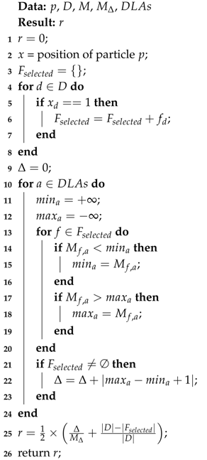
The inputs of Algorithm 1 are: p—The particle for which the fitness value is computed, D—The number of dimensions of the search space, M—A precomputed matrix, which is presented in more details next, M Δ —A metric used for the evaluation of that matrix, and  D L A s —The set of daily living activities monitored by the monitoring sensors. The output of the algorithm is r—The fitness value of the particle p.
Algorithm 1: The objective function of the adapted BPSO algorithm.
Applsci 10 01496 i001
Initially, the value of r is 0 (line 1), the value of x is equal to the position of the particle p (line 2) and  F s e l e c t e d is an empty set (line 3). For each d from the set { 1 , , D } , if the value of  x d is equal to 1 then the feature f d is included in the set of selected features F s e l e c t e d (lines 4–8). The initial value of  Δ is 0 (line 9). For each activity a from the set of daily living activities D L A s the steps from (lines 11–23) are repeated. The initial values of  m i n a and  m a x a are equal to + (line 11) and  (line 12). For each feature f from the set of features F s e l e c t e d , the values of  m i n a and  m a x a are updated in (lines 14–19) as follows: If the value of  M f , a is less than the value of  m i n a (line 14) then m i n a is initialized to the value of  M f , a (line 15) and if the value of  M f , a is greater than the value of  m a x a (line 17) then m a x a is initialized to the value of  M f , a (line 18). If F s e l e c t e d (line 21) then the value of  Δ is incremented with m a x a m i n a + 1 (line 22). In (line 25) the value of r is updated using the formula:
r = 1 2 × Δ M Δ + D F s e l e c t e d D .
The ideal value of r is 1 and corresponds to the case when Δ = M Δ and the number of selected features is 0, and the worst value of r is 0 and corresponds to the case when Δ = 0 and all features are selected. Consequently, r takes values from the interval [ 0 , 1 ] and the objective of the algorithm is to maximize that value. The algorithm returns the final value of r in (line 26).

3.6. Adapted BPSO Algorithm for Feature Selection in the Case of DLAs Sensors Data

The BPSO algorithm is adapted after the binary version of the PSO algorithm [35]. A method similar to the one presented in [36] is considered in order to the restrict the values of the positions of the particles to take values from the set { 0 , 1 } .
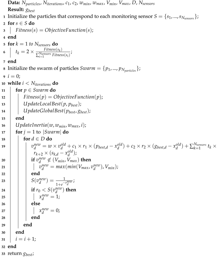
The inputs of the adapted BPSO Algorithm 2 are: N p a r t i c l e s —The number of particles, N i t e r a t i o n s —The maximum number of iterations, c 1 —The acceleration coefficient for the cognitive component, c 2 —The acceleration coefficient for the social component, w m i n — The minimum value for the inertia, w m a x —The maximum value for the inertia, V m i n —The minimum possible value for the velocity, V m a x —The maximum possible value for the velocity, D—The number of dimensions of the search space, and  N s e n s o r s — The number of monitoring sensors. The output g b e s t describes the position of the best particle after the maximum number of iterations N i t e r a t i o n s .
The adapted BPSO algorithm starts with the initialization of the particles that correspond to each monitoring sensor (line 1) and then for each particle that corresponds to a monitoring sensor, the corresponding fitness value is calculated (lines 2–4). Next, the weights of each sensor particle are computed (lines 5–7) in such a way that the weights are proportional to the fitness values of the sensor particles.
The particles swarm is initialized randomly (line 8) and the value of the initial iteration i is set to 0 in (line 9). The algorithm is then executed for a maximum number of iterations N i t e r a t i o n s given as input.
In each iteration for each particle from the swarm (lines 11–15), the fitness value is computed in (line 12) using the  O b j e c t i v e F u n c t i o n and the functions U p d a t e d L o c a l B e s t and  U p d a t e G l o b a l B e s t update the values of  p b e s t and  g b e s t as follows:
p b e s t = p if   F i t n e s s ( p ) > F i t n e s s ( p b e s t ) p b e s t otherwise
g b e s t = p b e s t if   F i t n e s s ( p b e s t ) > F i t n e s s ( g b e s t ) g b e s t otherwise .
The inertia is updated (line 16) considering the values of i, w m i n and  w m a x as follows:
w = w m a x if   i = 0 m a x ( w i , w m i n ) if   i > 0 .
Algorithm 2: Adapted BPSO Algorithm.
Applsci 10 01496 i002
Next, for each particle from the swarm (lines 17–30) and for each dimension of the particle (lines 18–29) the new value of the velocity of the particle for dimension d is computed, taking into consideration the following components:
  • the inertia component: w × v d o l d ,
  • the cognitive component: c 1 × r 1 × ( p b e s t , d x d o l d ) ,
  • the social component: c 2 × r 2 × ( g b e s t , d x d o l d ) ,
  • the sensors component: k = 1 N s e n s o r s t k × r k + 2 × ( s k , d x d o l d ) .
If the computed value is not in the interval ( V m i n , V m a x ) , then that value is updated either to V m i n or to V m a x (lines 20–22) as follows:
v d n e w = V m i n if   v d n e w < V m i n V m a x if   v d n e w > V m a x .
The velocity is converted into a probability value (line 23) using the exponential:
S ( v d n e w ) = 1 1 + e v d n e w .
In (lines 24–28) the value of a random value r 0 from [ 0 , 1 ] is applied in order to update the position of the particle as follows:
x d n e w = 1 if   r 0 < S ( v d n e w ) 0 otherwise .
In (line 31) the current iteration i is incremented with 1 and finally in (line 33) the algorithm returns the value of g b e s t .

4. Results

The adapted version of the BPSO algorithm was written and evaluated in Java in IntelliJ IDEA. The feature selection experiments for the adapted BPSO algorithm were performed in IntelliJ IDEA. The experiments for feature selection using FFS and BFE were performed in Konstanz Information Miner (KNIME) [37]. The experiments for feature selection using RF were performed in JetBrains PyCharm, using the sklearn library from Python. The experiments for feature selection based on the adapted versions of GA and DE were performed in IntelliJ IDEA. The properties of the system in which the experiments were performed are:
(1)
processor properties: Intel(R) Core(TM) i5-7600K CPU @ 3.80GHz 3.80 GHz;
(2)
installed memory (RAM) properties: 16.0 GB;
(3)
system type properties: 64-bit Operating System, x64-based processor.

4.1. Machine Learning Methodology for the Classification of DLAs Based on Adapted BPSO

The steps of the machine learning methodology that is applied in the classification of the DLAs using data generated by monitoring sensors are described in more details in the next subsections. In the Feature Selection step, the methodology integrates the algorithm that is presented in this article, namely the adapted BPSO algorithm. The methodology is also used as support in order to validate and to test this algorithm.

4.1.1. DLAs Sensors Data

In Figure 1, the placement of the monitoring sensors for the DaLiAc dataset is illustrated.
The main characteristics of the DaLiAc dataset are presented in Table 1.
In the case of the DaLiAc dataset the following activities are monitored:
(1)
D L A 1 —Sitting;
(2)
D L A 2 —Lying;
(3)
D L A 3 —Standing;
(4)
D L A 4 —Washing dishes;
(5)
D L A 5 —Vacuuming;
(6)
D L A 6 —Sweeping;
(7)
D L A 7 —Walking outside;
(8)
D L A 8 —Ascending stairs;
(9)
D L A 9 —Descending stairs;
(10)
D L A 10 —Treadmill running;
(11)
D L A 11 —Bicycling (50 watt);
(12)
D L A 12 —Bicycling (100 watt);
(13)
D L A 13 —Rope jumping;
The DaLiAc dataset contains information about 19 subjects (eight females and eleven males) aged 26 ± 8 years. The data was acquired using four SHIMMER (Shimmer Research, Dublin, Ireland) sensors. Each of those sensors is equipped with a triaxial accelerometer (three features) and a triaxial gyroscope (three features). The accelerometer measures the proper acceleration while the gyroscope measures the velocity and the angular velocity. The sensors were placed on the left ankle, on the right hip, on the chest and on the right ankle of the monitored subjects. The frequency of sampling of those sensors is 200 Hz.
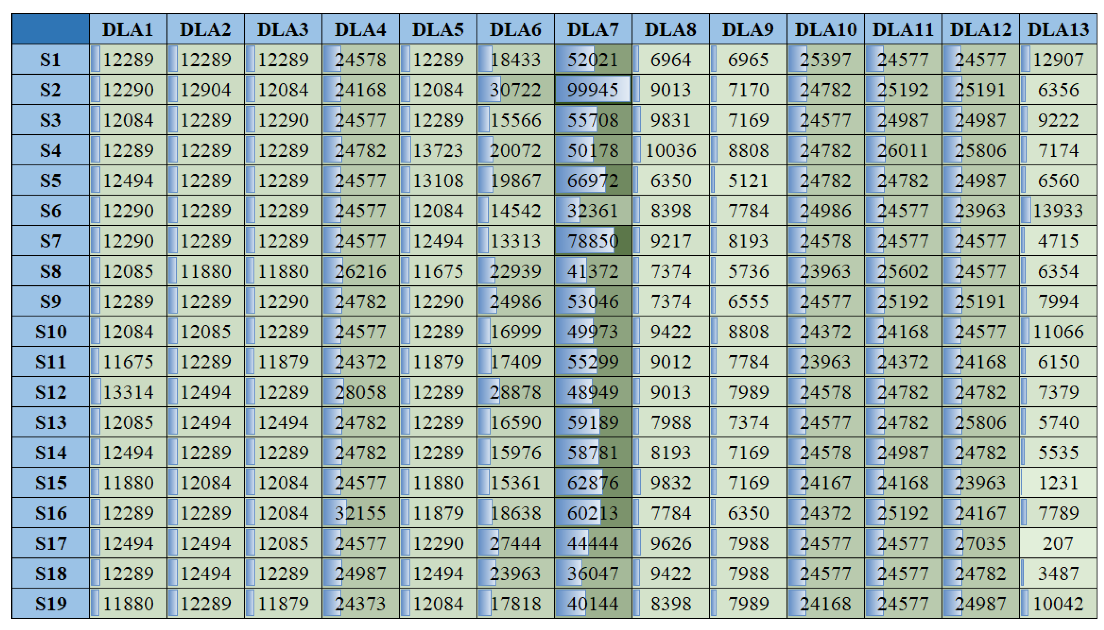
Figure 2 summarizes the number of samples of each daily living activity for each monitored subject. As can be seen in the figure, the walking outside activity ( D L A 7 ) contains the biggest number of samples for each monitored subject and moreover the samples for each activity are not balanced.

4.1.2. Feature Selection

In this step, various combinations of feature selection techniques are investigated. Four different types of feature selection techniques are applied:
(1)
The first technique considers the features that correspond to the monitoring sensors that are used for collecting the data from the monitoring sensors: six features (chest sensor), six features (right wrist sensor), six features (left ankle sensor), six features (right hip sensor);
(2)
The second technique considers the following three feature selection algorithms from literature: the forward feature selection (FFS) algorithm [38], the backward features elimination (BFE) algorithm [39] and the random forest (RF) [40];
(3)
The third technique considers the BPSO algorithm adapted for data generated by monitoring sensors placed on the bodies of the monitored subjects;
(4)
The fourth technique considers adapted versions of genetic algorithm (GA) [41] and differential evolution (DE) [42] for feature selection using the same objective function as in the case of the adapted BPSO algorithm;

4.1.3. Cross Validation

The approach presented in this article is based on 10-fold cross validation. Thus, the data is split randomly in 10 folds of approximately equal size and the prediction model is run 10 times, such that, in each run, the testing data is represented by a different fold from those 10 folds and the training data is represented by the remaining nine folds.

4.1.4. Machine Learning Classification Model

The machine learning classification model is used in the classification of the daily living activities performed by the monitored subjects based on the data from the monitoring sensors. The machine learning classification model that is applied in this article is RF. RF is an ensemble classification approach that is based on the development of a collection of decision trees and has applications in many domains, such as medicine, ecology, bioinformatics, astronomy, and agriculture, and, moreover, it is a very good option for imbalanced datasets.

4.1.5. DLAs Classification

The final output of the machine learning methodology is represented by the classified DLAs, considering the raw sensors data generated during the monitoring of the DLAs. The metrics that are applied in the evaluation of the models used for the classification of the DLAs are the recall, the precision, and the F-measure.

4.2. Feature Selection Results for DLAs Data Generated by Monitoring Sensors Using the Adapted BPSO Algorithm

The configuration of the parameters of the adapted BPSO algorithm applied in the experiments is summarized in Table 2.
The mappings between the sensor particles weights and the sensor positions for the DaLiAc dataset are: t 1 —C, t 2 —RW, t 3 —LA and t 4 —RH.
Table 3 summarizes the weights of the sensor particles for the DaLiAc Dataset, for each monitored subject.
In Table 4 is presented as a summary of the experiments for each monitored subject S, as follows: the mean running time in milliseconds t m , the mean fitness value f m , the mean number of returned features N R F m , and the mean accuracy a m . For each monitored subject, five experiments were performed. The value of N R F m is from { 5 , 6 , 7 , 8 } .
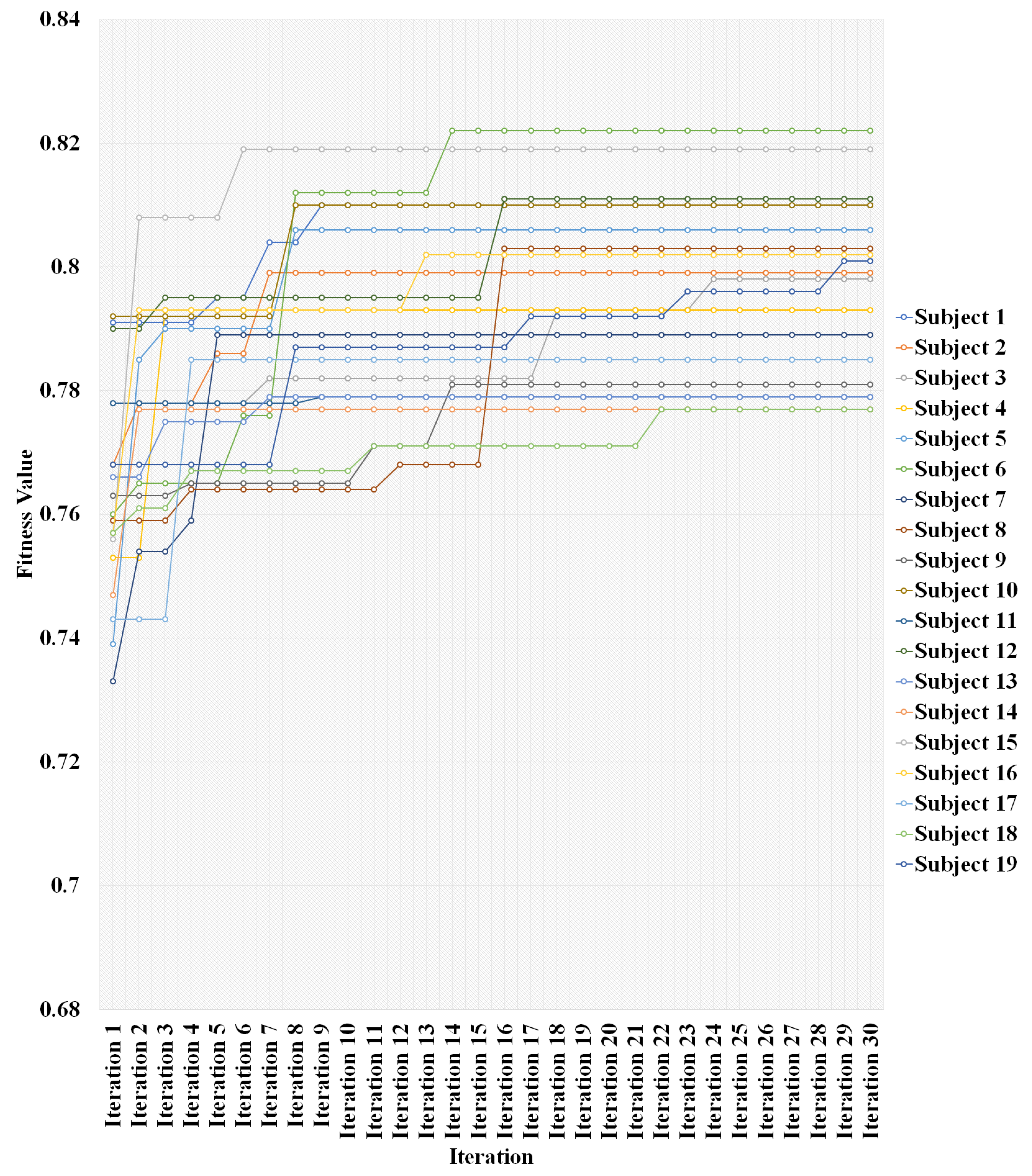
In Figure 3, the evolution of the fitness value in each iteration of the adapted BPSO algorithm for each subject is presented. The fitness value is improved after 30 iterations for each monitored subject.

4.3. Comparison of the Results Obtained Using the Adapted Version of BPSO for Feature Selection with the Results Obtained Using Other Methods

Both for the adapted versions of GA and DE for feature selection, the same objective function was applied as in the case of the adapted version of BPSO. Moreover, the number of returned features was restricted to six in the case of GA, DE, and BPSO, using the heuristic for features ranking introduced in this article, which returns the results presented in Appendix A. In the case of the adapted version of BPSO the configuration parameters described in the previous section were applied.
The following configurations are applied in the case of the other methods:
(1)
FFS and BFE—The standard configurations from KNIME, a threshold for the number of features equal to six and a random drawing strategy;
(2)
RF—The standard configurations from sklearn, a number of estimators equal to 1000, a maximum number of features equal to six;
(3)
GA—20 chromosomes, 30 iterations, C R (crossover rate) = 0.5 , M R (mutation rate) = 0.5 ;
(4)
DE—20 agents, 30 iterations, C R (crossover probability) = 0.5 , F (differential weight) = 1.0 .
Both for the adapted versions of GA and DE for feature selection, the same objective function was applied, as in the case of the adapted version of BPSO. Moreover, the number of returned features was restricted to six in the case of GA, DE, and BPSO, using the heuristic for features ranking introduced in this article that returns the results presented in Appendix A.
In Table 5, the running times for each feature selection approach are presented. The running time of BPSO is much better than the running time of BFE, GA and DE, but slightly worse than the running time of FFS and comparable to the running time of RF.
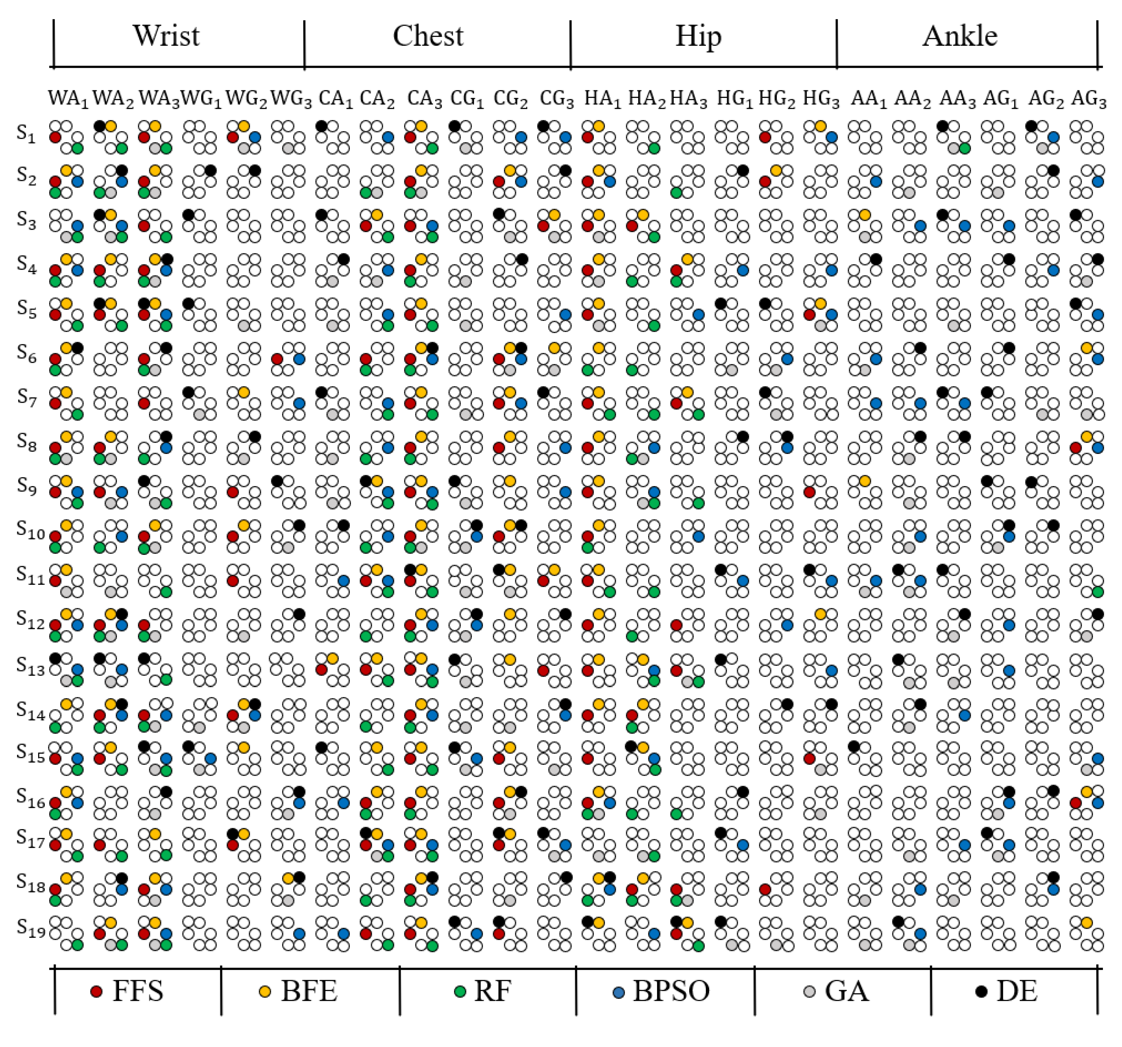
In Figure 4, the selected features for each feature selection approach are presented, namely FFS, BFE, RF, BPSO, GA, and DE, for each monitored subject.

4.4. Comparison of the DLAs Classification Results Obtained Using the Adapted Version of BPSO with the Results Obtained Using Other Methods

In Table 6 the DLAs classification results for each feature selection approach are presented, when the applied classification algorithm is RF. For eight out of the 19 monitored subjects, BPSO returns classification results that are from the top three results. Moreover, BPSO returns the best classification result in the case of the ninth monitored subject and this result is very promising, showing that further improvements of the algorithm might lead to even better classification results. Another promising observation is that GA returns the best classification result in the case of the fifteenth monitored subject and DE returns the best classification result in the case of the eighteenth monitored subject. Therefore, further improvements of the objective function and the application of other bio-inspired algorithms might lead to better classification results.

5. Discussion

In this section, a critical discussion and the main focus is on the following aspects is presented: (1) the results obtained when the adapted BPSO algorithm is applied for each type of DLA and (2) the comparison of the performance of the machine learning approach based on he BPSO algorithm with the performance of other approaches from the literature that consider the same benchmark dataset.

5.1. Application of Adapted BPSO Algorithm for DLAs Classification

The experiments were performed in KNIME as follows: the input data for each feature selection approach is read from an Excel Reader (XLS) node, the X-Partitioner node represents the beginning of the cross validation and it applies a number of validations equal to 10 and random sampling, two Number To String nodes are used for converting the data types of the labels of the samples from the training data and from the testing data from number to string, in order to prepare the data for classification, the Random Forest Learner node is used for creating a classification model and the split criterion is Information Gain Ration, the Random Forest Predictor node is used for predicting the results, considering the data resulted from the Random Forest Learner node and the testing data as input, one String to Number node is used for converting the data type of the predicted labels from string to number, the X-Aggregator node represents the end of the cross-validation, and finally the Scorer node is used for computing the accuracy.
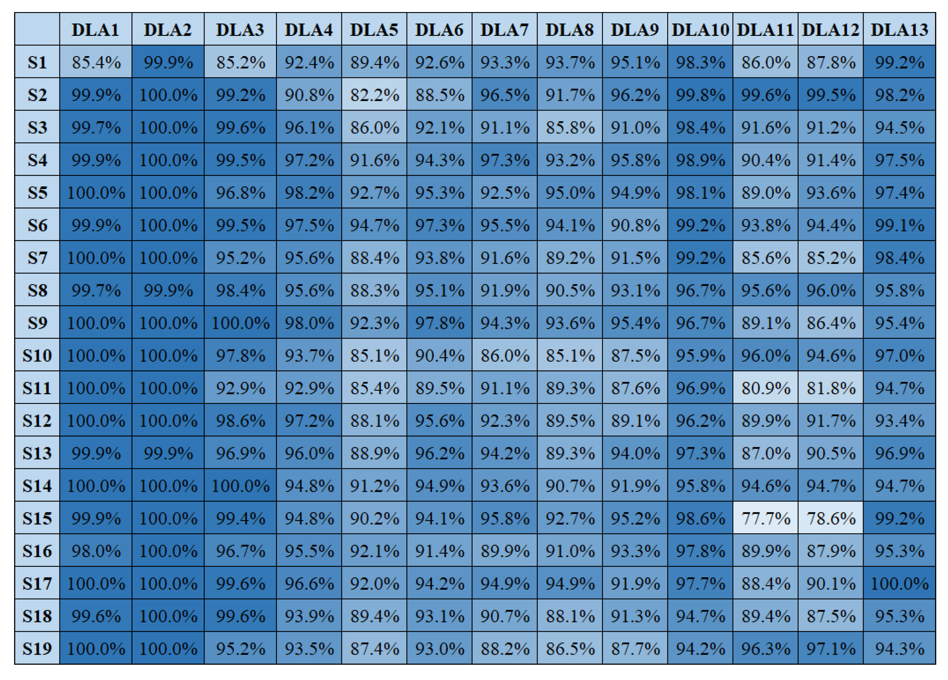
In Figure 5, the classification results for the DaLiAc Dataset for each monitored subject are presented. The best results were obtained in the case of the activities sitting ( D L A 1 ) and lying ( D L A 2 ) and the worst results were obtained in the case of the activities bicycling (50 watt) ( D L A 11 ) and bicycling (100 watt) ( D L A 12 ).

5.2. Comparison of the Performance of the BPSO Based Approach with the Performance of Literature Approaches

In this subsection, the results obtained using the machine learning methodology based on BPSO are compared with some of the best literature results. Table 7 presents a comparison of the results obtained, using the adapted version of the BPSO algorithm with the results obtained in the literature.
As can be seen in the table, the approach proposed in this article returns results comparable to the ones from the literature. The method presented in [33] returns much better results; however, in our approach we consider a maximum of six features and, in that approach, all features are used, therefore the two approaches are not directly comparable.

6. Conclusions

In this article, we presented a novel approach for feature selection in the case of data that is generated by sensors that monitor various types of DLAs. The method was tested and validated on the DaLiAc dataset. The experimental results show that the adapted version of BPSO presented in this article is comparable to other classical algorithms such as FFS, BFE, and RF, in terms of running time and classification performance.
The running time of the adapted version of BPSO is better than the running time of BFE and the developed objective function also returns promising results in combination with other bio-inspired algorithms, such as GA and DE. Moreover, for some monitored subjects the approach based on BPSO returns results that are much better than the ones obtained using classical algorithms for feature selection. Even if the proposed method based on BPSO returns results, which are not as good as the ones obtained using classical methods for some monitored subjects, further improvements of the objective function might lead to better results.
For example, the method presented in [33] performs significantly better,; however, it requires complex computational resources and image processing transformations.
As future research work the following research directions are proposed: (1) The testing and the validation of the proposed methodology using other validation types, such as the leave-one-subject validation type or the leave-two-subjects validation type, (2) the proposal of another heuristic for the ranking of the features returned by the adapted version of BPSO and (3) the comparison of the performance of the adapted version of BPSO with the performance of similar approaches based on other types of bio-inspired algorithms.

Author Contributions

Conceptualization, D.M., I.A. and T.C.; methodology, D.M. and T.C.; software, D.M. and I.A.; validation, D.M., I.A. and T.C.; formal analysis, I.S.; resources, I.A., T.C. and I.S.; writing–original draft preparation, D.M.; writing–review and editing, D.M., I.A. and T.C.; supervision, I.S.; project administration, I.A. and T.C.; funding acquisition, I.A., T.C. and I.S. All authors have read and agreed to the published version of the manuscript.

Funding

This research was funded by the Romanian National Authority for Scientific Research and Innovation, CCCDI–UEFISCDI and of the AAL Programme with co-funding from the European Union’s Horizon 2020 research and innovation programme grant number AAL59/2018 ReMIND within PNCDI III. The APC was funded by the Technical University of Cluj-Napoca through the grants for scientific research support programme.

Conflicts of Interest

The authors declare no conflict of interest.

Abbreviations

The following abbreviations are used in this manuscript:
AALambient assisted living
BFEbackward features elimination
BPSObinary particle swarm optimization
Cchest
CNNconvolutional neural network
CRcrossover rate or crossover probability
DaLiAcDaily Life Activities
DEdifferential evolution
DLAdaily living activity
ERTextremely randomized trees
Fdifferential weight
FFSforward feature selection
GAgenetic algorithm
k-NNk-nearest neighbor
KNIMEKonstanz Information Miner
HPSO-LShybrid particle swarm optimization with local search
HPSO-SSMhybrid particle swarm optimization with a spiral-shaped mechanism
ICTinformation and communication technology
IIinteraction information
IoTinternet of things
LAleft ankle
LRlogistic regression
MRmutation rate
NBnaive bayes
PSOparticle swarm optimization
PSO-LMparticle swarm optimization with learning memory
RFrandom forest
RHright hip
RSFSAIDrough-set-based feature selection algorithm for imbalanced data
RWright wrist
SVMsupport vector machine
UCIUniversity of California, Irvine
VAFvariance accounted for

Appendix A

The ranking of the features for each monitored subject S of the DaLiAc dataset in the adapted version of BPSO introduced in this article is presented next:
(1)
S 1 C A 1 , C A 3 , W A 3 , C A 2 , W A 1 , W A 2 , H A 3 , H A 1 , H A 2 , A A 3 , A A 2 , A A 1 , C G 3 , H G 3 , W G 2 , A G 1 , A G 2 , C G 2 , H G 2 , H G 1 , C G 1 , W G 3 , W G 1 , A G 3 ;
(2)
S 2 C A 1 , C A 3 , H A 3 , C A 2 , H A 1 , W A 3 , H A 2 , W A 1 , W A 2 , A A 2 , A A 3 , A A 1 , C G 3 , H G 3 , H G 1 , C G 1 , C G 2 , H G 2 , W G 2 , A G 1 , W G 3 , A G 2 , A G 3 , W G 1 ;
(3)
S 3 C A 1 , H A 3 , H A 2 , C A 2 , H A 1 , C A 3 , W A 1 , W A 3 , W A 2 , A A 3 , A A 2 , A A 1 , C G 3 , H G 3 , H G 1 , H G 2 , C G 2 , W G 2 , C G 1 , W G 3 , A G 1 , A G 2 , A G 3 , W G 1 ;
(4)
S 4 C A 1 , H A 2 , C A 3 , H A 1 , H A 3 , C A 2 , W A 1 , W A 3 , W A 2 , A A 3 , A A 2 , A A 1 , C G 3 , H G 3 , H G 1 , A G 1 , A G 3 , C G 2 , H G 2 , W G 2 , W G 3 , A G 2 , C G 1 , W G 1 ;
(5)
S 5 C A 1 , C A 3 , C A 2 , W A 3 , H A 3 , H A 2 , W A 1 , H A 1 , W A 2 , A A 3 , A A 2 , A A 1 , C G 3 , H G 3 , C G 2 , W G 2 , A G 1 , H G 2 , H G 1 , C G 1 , W G 3 , A G 2 , A G 3 , W G 1 ;
(6)
S 6 H A 3 , C A 1 , W A 3 , H A 2 , C A 3 , W A 1 , C A 2 , H A 1 , W A 2 , A A 3 , A A 2 , A A 1 , C G 3 , H G 3 , W G 2 , H G 2 , H G 1 , C G 2 , C G 1 , W G 3 , A G 1 , A G 2 , W G 1 , A G 3 ;
(7)
S 7 C A 1 , C A 3 , C A 2 , W A 1 , W A 3 , H A 1 , H A 3 , H A 2 , W A 2 , A A 3 , A A 2 , A A 1 , C G 3 , C G 1 , H G 3 , C G 2 , W G 2 , H G 1 , W G 3 , A G 1 , A G 2 , A G 3 , H G 2 , W G 1 ;
(8)
S 8 C A 1 , C A 3 , C A 2 , H A 2 , W A 3 , H A 1 , W A 1 , H A 3 , W A 2 , A A 3 , A A 2 , A A 1 , C G 3 , A G 1 , H G 3 , C G 2 , W G 2 , H G 1 , W G 3 , A G 2 , H G 2 , C G 1 , A G 3 , W G 1 ;
(9)
S 9 H A 3 , W A 1 , H A 1 , W A 3 , C A 1 , H A 2 , C A 3 , C A 2 , W A 2 , A A 2 , A A 3 , A A 1 , C G 3 , H G 3 , H G 2 , H G 1 , W G 2 , C G 2 , A G 1 , W G 3 , C G 1 , A G 3 , W G 1 , A G 2 ;
(10)
S 10 C A 1 , H A 3 , C A 3 , C A 2 , H A 2 , H A 1 , W A 1 , W A 3 , W A 2 , A A 3 , A A 2 , A A 1 , C G 3 , H G 3 , A G 1 , A G 2 , C G 2 , C G 1 , H G 1 , W G 3 , A G 3 , W G 2 , H G 2 , W G 1 ;
(11)
S 11 H A 3 , C A 1 , H A 2 , C A 3 , H A 1 , C A 2 , W A 3 , W A 2 , W A 1 , A A 3 , A A 2 , A A 1 , C G 3 , H G 3 , H G 1 , C G 1 , A G 1 , A G 2 , H G 2 , W G 2 , W G 3 , C G 2 , A G 3 , W G 1 ;
(12)
S 12 C A 3 , C A 1 , C A 2 , H A 3 , W A 3 , W A 1 , H A 1 , H A 2 , W A 2 , A A 3 , A A 2 , A A 1 , C G 3 , C G 1 , C G 2 , W G 2 , H G 3 , W G 3 , A G 1 , H G 1 , H G 2 , A G 3 , A G 2 , W G 1 ;
(13)
S 13 C A 1 , C A 2 , C A 3 , H A 1 , H A 3 , H A 2 , W A 3 , W A 1 , W A 2 , A A 3 , A A 2 , A A 1 , C G 3 , A G 1 , H G 1 , H G 3 , C G 1 , C G 2 , W G 2 , A G 2 , W G 3 , A G 3 , H G 2 , W G 1 ;
(14)
S 14 H A 3 , C A 1 , H A 2 , H A 1 , W A 3 , C A 3 , W A 1 , C A 2 , W A 2 , A A 3 , A A 2 , A A 1 , H G 3 , C G 3 , H G 1 , W G 2 , H G 2 , W G 3 , A G 1 , C G 2 , A G 2 , C G 1 , A G 3 , W G 1 ;
(15)
S 15 C A 1 , C A 2 , H A 3 , C A 3 , W A 3 , W A 1 , W A 2 , H A 2 , H A 1 , A A 2 , A A 3 , A A 1 , C G 3 , A G 1 , C G 1 , W G 2 , H G 3 , W G 3 , C G 2 , H G 1 , H G 2 , W G 1 , A G 3 , A G 2 ;
(16)
S 16 C A 1 , H A 1 , H A 2 , H A 3 , C A 2 , C A 3 , W A 3 , W A 1 , W A 2 , A A 2 , A A 3 , A A 1 , C G 3 , H G 1 , A G 3 , C G 1 , H G 3 , A G 1 , C G 2 , W G 2 , H G 2 , W G 3 , A G 2 , W G 1 ;
(17)
S 17 C A 1 , C A 3 , C A 2 , H A 2 , W A 3 , W A 1 , W A 2 , H A 1 , H A 3 , A A 2 , A A 3 , A A 1 , C G 3 , H G 3 , H G 1 , W G 2 , A G 1 , C G 2 , C G 1 , W G 3 , A G 3 , A G 2 , W G 1 , H G 2 ;
(18)
S 18 C A 1 , H A 3 , H A 1 , C A 2 , H A 2 , C A 3 , W A 3 , W A 1 , W A 2 , A A 3 , A A 2 , A A 1 , C G 3 , H G 3 , H G 1 , C G 2 , W G 2 , A G 1 , H G 2 , A G 3 , A G 2 , W G 3 , C G 1 , W G 1 ;
(19)
S 19 C A 1 , C A 2 , H A 3 , H A 2 , C A 3 , W A 1 , W A 3 , H A 1 , W A 2 , A A 3 , A A 2 , A A 1 , C G 3 , H G 3 , H G 1 , H G 2 , C G 2 , C G 1 , W G 2 , A G 2 , A G 1 , W G 3 , A G 3 , W G 1 ;

References

  1. ReMIND. Available online: https://www.aalremind.eu/ (accessed on 15 January 2020).
  2. Moldovan, D.; Anghel, I.; Cioara, T.; Salomie, I.; Chifu, V.; Pop, C. Kangaroo mob heuristic for optimizing features selection in learning the daily living activities of people with Alzheimer’s. In Proceedings of the 22nd International Conference on Control Systems and Computer Science (CSCS), Bucharest, Romania, 28–30 May 2019; pp. 236–243. [Google Scholar]
  3. Schneider, C.; Trukeschitz, B.; Rieser, H. Measuring the use of the active and assisted living prototype CARIMO for home care service users: Evaluation framework and results. Appl. Sci. 2020, 10, 38. [Google Scholar] [CrossRef] [Green Version]
  4. Maskeliunas, R.; Damasevicius, R.; Segal, S. A review of internet of things technologies for ambient assisted living environments. Future Internet 2019, 11, 259. [Google Scholar] [CrossRef] [Green Version]
  5. Dziak, D.; Jachimczyk, B.; Kulesza, W.J. IoT-based information system for healthcare application: Design methodology approach. Appl. Sci. 2017, 7, 596. [Google Scholar] [CrossRef]
  6. Terashi, H.; Mitoma, H.; Yoneyama, M.; Aizawa, H. Relationship between amount of daily movement measured by a triaxial accelerometer and motor symptoms in patients with Parkinson’s disease. Appl. Sci. 2017, 7, 486. [Google Scholar] [CrossRef] [Green Version]
  7. Samie, F.; Bauer, L.; Henkel, J. From cloud down to things: An overview of machine learning in internet of things. IEEE Internet Things J. 2019, 6, 4921–4934. [Google Scholar] [CrossRef]
  8. Vitabile, S.; Marks, M.; Stojanovic, D.; Pllana, S.; Molina, J.M.; Krzyszton, M.; Sikora, A.; Jarynowski, A.; Hosseinpour, F.; Jakobik, A.; et al. Medical data processing and analysis for remote health and activities monitoring. In High-Performance Modelling and Simulation for Big Data Applications: Selected Results of the COST Action IC1406 cHiPSet; Kolodziej, J., Gonzalez-Velez, H., Eds.; Springer International Publishing: Cham, Switzerland, 2019; pp. 186–220. [Google Scholar]
  9. Chelli, A.; Patzold, M. A machine learning approach for fall detection and daily living activity recognition. IEEE Access 2019, 7, 38670–38687. [Google Scholar] [CrossRef]
  10. Saadeh, W.; Butt, S.A.; Altaf, M.A.B. A patient-specific single sensor IoT-based wearable fall prediction and detection system. IEEE Trans. Neural Syst. Rehabil. Eng. 2019, 5, 995–1003. [Google Scholar] [CrossRef] [PubMed]
  11. Yatbaz, H.Y.; Eraslan, S.; Yesilada, Y.; Ever, E. Activity recognition using binary sensors for elderly people living alone: Scanpath trend analysis approach. IEEE Sens. J. 2019, 19, 7575–7582. [Google Scholar] [CrossRef]
  12. Awais, M.; Chiari, L.; Ihlen, E.A.F.; Helbostad, J.; Palmerini, L. Physical activity classification for elderly people in free-living conditions. IEEE J. Biomed. Health 2019, 23, 197–207. [Google Scholar] [CrossRef] [PubMed]
  13. Yahaya, S.W.; Lotfi, A.; Mahmud, M. A consensus novelty detection ensemble approach for anomaly detection in activities of daily living. Appl. Soft Comput. 2019, 83, 105613. [Google Scholar] [CrossRef]
  14. Uddin, M.Z.; Hassan, M.M.; Alsanad, A.; Savaglio, C. A body sensor data fusion and deep recurrent neural network-based behavior recognition approach for robust healthcare. Inform. Fusion 2020, 55, 105–115. [Google Scholar] [CrossRef]
  15. De-La-Hoz-Franco, E.; Ariza-Colpas, P.; Quero, J.M.; Espinilla, M. Sensor-based datasets for human activity recognition—A systematic review of literature. IEEE Access 2018, 6, 59192–59210. [Google Scholar] [CrossRef]
  16. Leutheuser, M.; Schludhaus, D.; Eskofier, B.M. Hierarchical, multi-sensor based classification of daily life activities: Comparison with state-of-the-art algorithms using a benchmark dataset. PLoS ONE 2013, 8. [Google Scholar] [CrossRef] [PubMed] [Green Version]
  17. Lin, Q.; Liu, S.; Zhu, Q.; Tang, C.; Song, R.; Chen, J.; Coello, C.A.; Wong, K.-C.; Zhang, J. Particle swarm optimization with a balanceable fitness estimation for many-objective optimization problems. IEEE Trans. Evolut. Comput. 2018, 22, 32–46. [Google Scholar] [CrossRef]
  18. Zhou, P.; Hu, X.; Li, P.; Wu, X. Online feature selection for high-dimensional class-imbalanced data. Knowl. Based Syst. 2017, 136, 187–199. [Google Scholar] [CrossRef]
  19. Liu, M.; Xu, C.; Luo, Y.; Xu, C.; Wen, Y.; Tao, D. Cost-sensitive feature selection by optimizing F-measures. IEEE Trans. Image Process. 2018, 27, 1323–1335. [Google Scholar] [CrossRef] [PubMed] [Green Version]
  20. Maldonado, S.; Lopez, J. Dealing with high-dimensional class-imbalanced datasets: Embedded feature selection for SVM classification. Appl. Soft Comput. 2018, 67, 94–105. [Google Scholar] [CrossRef]
  21. Xu, Y. Maximum margin of twin spheres support vector machine for imbalanced data classification. IEEE Trans. Cybern. 2017, 47, 1540–1550. [Google Scholar] [CrossRef] [PubMed]
  22. Chen, H.; Li, T.; Fan, X.; Luo, C. Feature selection for imbalanced data based on neighborhood rough sets. Inform. Sci. 2019, 483, 1–20. [Google Scholar] [CrossRef]
  23. Hosseini, E.S.; Moattar, M.H. Evolutionary feature subsets selection based on interaction information for high dimensional imbalanced data classification. Appl. Soft Comput. 2019, 82, 105581. [Google Scholar]
  24. Xue, B.; Zhang, M.; Browne, W.N. Particle swarm optimisation for feature selection in classification: Novel initialisation and updating mechanisms. Appl. Soft Comput. 2014, 18, 261–276. [Google Scholar]
  25. Moradi, P.; Gholampour, M. A hybrid particle swarm optimization for feature subset selection by integrating a novel local search strategy. Appl. Soft Comput. 2016, 43, 117–130. [Google Scholar]
  26. Samanthula, B.K.; Elmehdwi, Y.; Jiang, W. K-nearest neighbor classification over semantically secure encrypted relational data. IEEE T Knowl. Data Eng. 2015, 27, 1261–1273. [Google Scholar]
  27. Wei, B.; Zhang, W.; Xia, X.; Zhang, Y.; Yu, F.; Zhu, Z. Efficient feature selection algorithm based on particle swarm optimization with learning memory. IEEE Access 2019, 7, 166066–166078. [Google Scholar]
  28. Xiong, B.; Li, Y.; Huang, M.; Shi, W.; Du, M.; Yang, Y. Feature selection of input variables for intelligence joint moment prediction based on binary particle swarm optimization. IEEE Access 2019, 7, 182289–182295. [Google Scholar]
  29. Chen, K.; Zhou, F.-Y.; Yuan, X.-F. Hybrid particle swarm optimization with spiral-shaped mechanism for feature selection. Expert Syst. Appl. 2019, 128, 140–156. [Google Scholar]
  30. Casale, P.; Altini, M.; Amft, O. Transfer learning in body sensor networks using ensembles of randomized trees. IEEE Internet Things 2015, 2, 33–40. [Google Scholar]
  31. Nazabal, A.; Garcia-Moreno, P.; Artes-Rodriguez, A.; Ghahramani, Z. Human activity recognition by combining a small number of classifiers. IEEE J. Biomed. Health 2016, 20, 1342–1351. [Google Scholar]
  32. Zdravevski, E.; Lameski, P.; Trajkovik, V.; Kulakov, A.; Chorbev, I.; Goleva, R.; Pombo, N.; Garcia, N. Improving activity recognition accuracy in ambient-assisted living systems by automated feature engineering. IEEE Access 2017, 5, 5262–5280. [Google Scholar]
  33. Hur, T.; Bang, J.; Huynh-The, T.; Lee, J.; Kim, J.-I.; Lee, S. Iss2Image: A novel signal-encoding technique for CNN-based human activity recognition. Sensors 2018, 18, 3910. [Google Scholar]
  34. Kumar, A.; Kim, J.; Lyndon, D.; Fulham, M.; Feng, D. An ensemble of fine-tuned convolutional neural networks for medical image classification. IEEE J. Biomed. Health 2017, 21, 31–40. [Google Scholar]
  35. Liu, J.; Mei, Y.; Li, X. An analysis of the inertia weight parameter for binary particle swarm optimization. IEEE Trans. Evolut. Comput. 2016, 20, 666–681. [Google Scholar]
  36. Too, J.; Abdullah, A.R.; Saad, N.M. A new co-evolution binary particle swarm optimization with multiple inertia weight strategy for feature selection. Informatics 2019, 6, 21. [Google Scholar]
  37. Feltrin, L. KNIME an open source solution for predictive analytics in the geosciences [Software and Data Sets]. IEEE Geosci. Remote Sens. Mag. 2015, 3, 28–38. [Google Scholar]
  38. Macedo, F.; Oliveira, M.R.; Pacheco, A.; Valadas, R. Theoretical foundations of forward feature selection methods based on mutual information. Neurocomputing 2019, 325, 67–89. [Google Scholar]
  39. Maldonado, S.; Weber, R.; Famili, F. Feature selection for high-dimensional class-imbalanced data sets using support vector machines. Inform. Sci. 2014, 286, 228–246. [Google Scholar]
  40. Bader-El-Den, M.; Teitei, E.; Perry, T. Biased random forest for dealing with the class imbalance problem. IEEE Trans. Neural Netw. Learn. Syst. 2019, 30, 2163–2172. [Google Scholar]
  41. Alirezazadeh, P.; Fathi, A.; Abdali-Mohammadi, F. A genetic algorithm-based feature selection for kinship verification. IEEE Signal Process. Lett. 2015, 22, 2459–2463. [Google Scholar]
  42. Zhang, Y.; Gong, D.-W.; Gao, X.-Z.; Tian, T.; Sun, X.-Y. Binary differential evolution with self-learning for multi-objective feature selection. Inform. Sci. 2020, 507, 67–85. [Google Scholar]
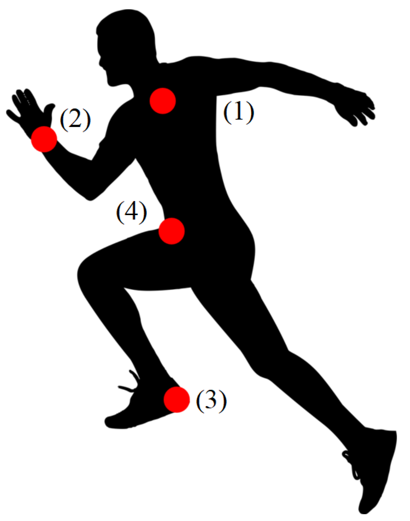
Figure 1. Sensors positions for the Daily Life Activities (DaLiAc) dataset: (1) chest (C), (2) right wrist (RW), (3) left ankle (LA), (4) right hip (RH).
Applsci 10 01496 g001
Figure 2. Distribution of DLAs samples for each monitored subject of the DaLiAc dataset.
Applsci 10 01496 g002
Figure 3. Fitness value evolution in each iteration of the adapted BPSO algorithm for the best results.
Applsci 10 01496 g003
Figure 4. Selected features for: (1) FFS, (2) BFE, (3) RF, (4) BPSO, (5) GA, and (6) DE.
Applsci 10 01496 g004
Figure 5. The DLAs precision results for the DaLiAc dataset using adapted BPSO and RF for each monitored subject.
Applsci 10 01496 g005
Table 1. DaLiAc dataset characteristics.
CharacteristicValue
number of daily living activities (DLAs)13
number of subjects19
number of monitoring sensors4
total number of features24
sampling frequency200 Hz
Table 2. Configuration of the adapted binary particle swarm optimization (BPSO) algorithm parameters.
ParameterSignificanceValue
N i t e r a t i o n s number of iterations30
N p a r t i c l e s number of particles20
c 1 cognitive component value2
c 2 social component value2
V m i n minimum value of velocity 0.5
V m a x maximum value of velocity 0.5
w m i n minimum value of inertia 0.500
w m a x maximum value of inertia 0.901
Table 3. Sensor particle weights for the DaLiAc dataset for each monitored subject.
Monitored Subject/Sensor Particle Weight t 1 t 2 t 3 t 4
S 1 0.4780.5670.4480.507
S 2 0.5440.4900.4660.500
S 3 0.5700.5350.4180.477
S 4 0.4980.5590.4700.473
S 5 0.5650.4920.4650.478
S 6 0.4820.5290.4650.524
S 7 0.4720.5020.5280.498
S 8 0.5640.5200.4350.481
S 9 0.5370.5540.4290.480
S 10 0.5090.5050.4720.514
S 11 0.5080.4940.4610.537
S 12 0.5360.5200.4740.470
S 13 0.5940.5100.4410.455
S 14 0.5550.4800.4750.490
S 15 0.4970.5250.4890.489
S 16 0.5730.4900.4500.487
S 17 0.5550.5270.4510.467
S 18 0.5710.4840.4530.492
S 19 0.5320.5240.4720.472
Table 4. Summary of the adapted BPSO algorithm mean results for each monitored subject.
Subject t m f m NRF m a m
S 1 684,4760.8188 91.0 %
S 2 910,0640.8066 93.7 %
S 3 739,9850.7957 92.4 %
S 4 714,8690.7997 90.0 %
S 5 726,9320.8117 90.4 %
S 6 614,4170.8147 94.3 %
S 7 733,8000.7965 86.0 %
S 8 625,1660.8087 91.1 %
S 9 665,9250.8007 93.3 %
S 10 658,8370.8046 89.7 %
S 11 761,4300.8027 88.2 %
S 12 793,3770.8037 92.8 %
S 13 802,2590.7987 92.1 %
S 14 760,7300.8036 90.9 %
S 15 813,8280.8117 90.7 %
S 16 885,9000.8057 91.0 %
S 17 875,1750.7986 92.7 %
S 18 774,2230.7937 91.1 %
S 19 753,1610.7986 91.7 %
Table 5. The running time for forward feature selection (FFS), backward features elimination (BFE), random forest (RF), binary particle swarm optimization (BPSO), genetic algorithm (GA) and differential evolution (DE) for each monitored subject, in milliseconds.
Subject/Features SelectionFFSBFERFBPSOGADE
S 1 333,8422,517,009914,742636,9301,930,8861,282,519
S 2 409,8655,253,3601,117,351953,3762,213,7811,519,955
S 3 333,8723,661,512800,075799,1511,766,3701,271,330
S 4 337,0704,481,319751,205716,9611,787,1771,269,005
S 5 348,0891,632,155886,658703,2761,836,6031,316,106
S 6 309,6791,569,169680,149658,8941,613,0771,146,485
S 7 368,9061,704,399827,109705,6061,882,5461,373,507
S 8 326,1911,540,248863,979588,2801,663,4401,207,692
S 9 349,5034,865,604723,893652,3141,791,7081,282,526
S 10 345,8903,366,558695,436575,5861,750,7481,285,746
S 11 329,9802,669,384814,888822,1931,733,9391,255,230
S 12 342,6861,580,970830,055868,9761,832,4321,319,197
S 13 336,9754,311,050905,903849,8421,855,3741,294,919
S 14 333,7463,019,609902,391892,8801,761,7301,253,549
S 15 326,0563,081,598873,733915,9391,648,9311,233,069
S 16 349,3413,455,5771,109,170931,5241,838,8681,303,958
S 17 322,2971,534,359730,817664,4681,715,6161,287,910
S 18 318,7425,478,390715,003875,0471,644,8041,157,746
S 19 319,6284,515,086782,075675,7791,662,0811,141,452
Table 6. The random forest accuracy classification results for each feature selection approach for the DaLiAc dataset for each monitored subject 1 .
Subject/Features SelectionCRWLARHFFSBFERFBPSOGADE
S 1 90.9 % 93.7 % 87.1% 89.2 % 91.7 % 92.8% 91.5 % 92.1 % ̲ ̲ ̲ 91.5 % 90.1 %
S 2 94.1 % 97.1%88.8% 90.6 % 97.5 % 97.5 % 97.0 % ̲ ̲ ̲ 95.8 % 96.8 % 94.2 %
S 3 91.9 % 94.0 % 86.7% 90.3 % 93.0 % ̲ ̲ ̲ 93.4% 94.0 % 93.4%93.4% 92.7 %
S 4 90.5 % 96.2 % 87.5% 89.5 % 95.9%95.9% 95.4 % 95.7 % ̲ ̲ ̲ 93.5 % 91.2 %
S 5 92.1 % 95.4 % 82.3% 90.7 % 95.3%95.3% 94.9 % ̲ ̲ ̲ 94.7 % 88.8 % 93.6 %
S 6 95.5 % ̲ ̲ ̲ 94.1 % 88.3% 93.3 % 95.1 % 96.8 % 95.4 % 96.6% 93.2 % 94.4 %
S 7 94.6 % 95.0 % ̲ ̲ ̲ 87.1% 93.0 % 96.1 % 95.7% 94.5 % 92.5 % 91.9 % 91.2 %
S 8 92.1 % 93.9 % 85.5% 88.3 % 96.9 % 96.9 % 95.8% 95.1 % ̲ ̲ ̲ 93.8 % 88.7 %
S 9 92.3 % 93.4 % 83.6% 88.2 % 94.4% 94.3 % ̲ ̲ ̲ 94.0 % 94.7 % 89.6 % 94.0 %
S 10 94.5% 94.1 % ̲ ̲ ̲ 87.0% 88.4 % 95.0 % 95.0 % 94.5% 92.4 % 93.7 % 90.0 %
S 11 91.7 % 91.4 % 84.7% 88.6 % 92.1% 91.9 % ̲ ̲ ̲ 92.7 % 90.4 % 88.9 % 89.3 %
S 12 94.3 % 94.1 % 85.1% 90.5 % 94.6% 95.6 % 94.5 % ̲ ̲ ̲ 94.0 % 93.3 % 94.5 % ̲ ̲ ̲
S 13 92.6 % 94.1 % 86.0% 89.8 % 93.2 % ̲ ̲ ̲ 92.8 % 91.9 % 94.0% 91.4 % 91.4 %
S 14 91.4 % 95.6%86.3% 91.3 % 95.4 % ̲ ̲ ̲ 95.9 % 95.1 % 95.0 % 90.9 % 94.1 %
S 15 91.6 % 93.2%88.8% 91.7 % 93.0 % ̲ ̲ ̲ 93.3 % 91.2 % 92.5 % 93.3 % 90.0 %
S 16 91.5 % 91.6 % ̲ ̲ ̲ 81.3% 90.1 % 94.2 % 94.2 % 91.5 % 92.8% 91.2 % 89.3 %
S 17 95.1 % 95.3 % ̲ ̲ ̲ 89.2% 94.5 % 95.8% 95.9 % 94.4 % 94.5 % 92.8 % 95.0 %
S 18 89.0 % 93.3 % ̲ ̲ ̲ 83.6% 88.1 % 93.5%93.5% 91.1 % 92.6 % 88.7 % 93.9 %
S 19 92.1 % 96.0 % ̲ ̲ ̲ 88.4% 92.2 % 96.2% 97.0 % 96.2% 93.4 % 92.9 % 91.2 %
Average 92.5 % 94.2 % ̲ ̲ ̲ 86.1% 90.4 % 94.6% 94.9 % 93.9 % 93.8 % 92.0 % 92.0 %
1 (1) The best results are underlined with one line, (2) the second best results are underlined with two lines, (3) the third best results are underlined with three lines, (4) the worst results are underlined with one dash line.
Table 7. Comparison of the results obtained using the adapted version of the BPSO algorithm with the results obtained in the literature using the DaLiAc dataset as the experimental support.
ApproachResultMethod
Our approach 93.8 % accuracyThe features are selected using an adapted version of BPSO and the data is classified using RF
(Zdravevski et al. [32]) 93.4 % accuracyA method that applies the score-drift feature selection, based on an algorithm for feature extraction, selection, and classification
(Leutheuser et al. [16]) 89.6 % accuracyA hierarchical multi-sensor based classification system
(Hur et al. [33]) 96.4 % accuracyA method that is based on Iss2Image-UCNet6