Structural Topology Design Optimization Using the Binary Bat Algorithm

Abstract

In this study, the binary bat algorithm (BBA) for structural topology optimization is implemented. The problem is to find the stiffest structure using a certain amount of material and some constraints using the bit-array representation method. A new filtering algorithm is proposed to make BBA find designs with no separated objects, no checkerboard patterns, less unusable material, and higher structural performance. A volition penalty function for topology optimization is also proposed to accelerate the convergence toward the optimal design. The main effect of using the BBA lies in the fact that the BBA is able to handle a large number of design variables in comparison with other well-known metaheuristic algorithms. Based on the numerical results of four benchmark problems in structural topology optimization for minimum compliance, the following conclusions are made: (1) The BBA with the proposed filtering algorithm and penalty function are effective in solving large-scale numerical topology optimization problems (fine finite elements mesh). (2) The proposed algorithm produces solid-void designs without gray areas, which makes them practical solutions that are applicable in manufacturing.

1. Introduction

Structural optimization is considered as one of the most important fields in engineering because it can propose innovative designs that satisfy different multidiscipline design requirements. There are three kinds of structural optimization: geometry, size, and topology. Geometry optimization involves finding the best arrangement of the joints. In size optimization, the main goal is to find the dimensions of the elements where the locations of the joints are fixed. Structural topology optimization is used to determine the best number, location, and size of voids as well as the best connectivity of the design domain. For any structural topology optimization problem, the applied loads, the support condition, the possible design requirements or any other restrictions, and the volume of structure to be constructed are the only known quantities. Then, in an iterative manner, the material is redistributed to meet the design requirements [1].

Structural topology optimization methods have received much attention in the relevant literature. They have been improved because they are very attractive for use in many industrial applications in civil and mechanical engineering [2]. These methods can help designers select suitable structures and reduce the effort required by trial and error. In structural topology optimization, similar to any other type of optimization, two methods are used: the deterministic (i.e., calculus-based or gradient-based) method and stochastic (i.e., metaheuristic or nature-inspired) algorithms.

In the deterministic method, the Solid Isotopic Microstructure with Penalization (SIMP) or the power law method introduced by Bendsøe [1] is a generally accepted and efficient tool for structural topology optimization. In the SIMP method, the design variables are the density of each element, and the material property of each element is constant [3]. The gradient-based SIMP method is used to search for the optimum point in the neighborhood of the current estimate. It tends to converge to a local optimum with a blurry boundary. Moreover, the SIMP method cannot directly solve 0/1 problems, so it requires a filtering method to resolve the final design [4,5,6]. The Canonical Duality Theory (CDT) developed by Gao [7] is used to analytically solve structural topology optimization problems with solid or void material distribution. The numerical results of solving benchmark topology optimization problems showed that the CDT method is powerful in comparison with SIMP and Basic Evolutionary Structural Optimization (BESO) methods in terms of computational time, the final compliance, not generating grayscale areas, and fewer checkerboard patterns [8,9,10]. For problems with mesh sizes of 180 × 60 and 150 × 50, the CDT method showed some checkerboard patterns. Rational Approximation of Material Properties (RAMP) developed by Stolpe and Svanberg [11] and the generalized form of it (called GRAMP) were used to solve two benchmark topology optimization problems for minimum compliance. Using a penalization factor of value equal to 3, Dzierżanowski showed that GRAMP was able to produce an almost “0–1” layout of material [12]. In comparison with the SIMP method, GRAMP and RAMP were able to obtain designs with fewer grayscale areas and better compliance. However, GRAMP and RAMP were not able to produce exactly void/solid material distribution. In addition to the compliance minimization topology design methods, the stress-constrained topology optimization methods have received much attention since the pioneering work of Duysinx and Bendsøe [13]. It involves stress-related objectives or constraints to overcome three main issues in the minimizing compliance design: highly non-linear stress behavior, the local nature of stress constraints, and the stress singularity [14,15,16]. Similar to the compliance topology optimization approaches, the stress-constrained topology optimization methods search locally, and final designs can have blurry boundaries or checkerboard patterns depending on an exponent factor.

The deterministic approach described in the preceding paragraph requires gradient information of functions. The other fundamental approach to topology optimization is to use metaheuristic methods [17]. Over the last few decades, many metaheuristic optimization algorithms have been explored to solve complex optimization problems. These methods are based on simulations, and they do not require gradient information. Based on the number of solutions in each iteration, there are two types of metaheuristic: (1) single solution-based, such as the Simulating Annealing (SA) and Harmony Search (HS) algorithms, and (2) population-based, such as the Genetic Algorithm (GA). Based on the inspiration, metaheuristic algorithms can be categorized into four types: evolutionary algorithms, such as GA and the Covariance Matrix Adaptation Evolution Strategy (CMA-ES) [18,19], physical-based, such as Colliding Bodies (CB), human-based, such as Tabu Search (TS), and swarm intelligence, such as Particle Swarm Optimization (PSO) [20]. All types of metaheuristic algorithms have common features: the search in the entire design space, two searching phases—exploration and exploitation, the use of random numbers to generate new designs, and no good initial designs are required. Metaheuristic algorithms are suitable for tackling many real-life optimization problems, especially those having many local minimum designs or those in which it is not possible to calculate the gradient information of the problem. Like gradient-based algorithms, metaheuristic algorithms have some drawbacks. That is, depending on the number of design variables and the range of each design, they may require many function evaluations to obtain a reasonable solution in comparison with gradient-based optimization algorithms because the number of possible combinations drastically increases. However, this computation efficiency comparison may not be meaningful because the gradient-based approach is a local search method, and the problem of global optimization requires all local optimal solutions. Thus, the deterministic approach may become as computationally expensive as metaheuristic algorithms are [4].

The Bat Algorithm (BA) is based on observations of a natural phenomenon. It was inspired by the echo locative behavior of bats. In the BA, artificial bats ($n$ designs of dimension $d$) are search agents mimicking the search nature of real bats using loudness and emission rates. Regarding some benchmark continuous design variable optimization problems, such as Rosenbrok’s ($d=16$) and Schwefel’s ($d=128$), it was proven that the BA is capable of obtaining competitive results in comparison with other well-known metaheuristic algorithms, such as GA and PSO [21]. The BA has also been used to solve some discrete design variables optimization problems, such as the symmetric and asymmetric traveling salesman problems [22] and steel frames subjected to American Institute of Steel Construction-Allowable Stress Design (AISC-ASD) design requirements [23]. The binary version of the BA was developed by Mirjalili et al. [24], who termed it the Binary Bat Algorithm (BBA). The BBA has been used to solve 22 benchmark functions. The results have shown that the BBA was able to surpass the binary PSO and GA in terms of the quality of the solutions and the total number of function evaluations required to reach the optimal design [24].

Metaheuristic algorithms for topology optimization usually use binary code (i.e., 0/1) to represent void/solid material distribution. Thus, they can be used directly to solve structural topology optimization problems because no gray area is generated. Although a great advantage over gradient-based topology optimization algorithms, in addition to the advantages mentioned above, metaheuristic algorithms are generally less efficient than mathematical programming methods [4,5,11]. GA has been used to solve topology optimization problems for more than three decades [5,11,12,13,14]. Kaveh et al. [15] used the Ant Colony methodology for the topology optimization of structures to find the stiffest structures based on the element’s contribution to the strain energy. Wu and Tseng [3] modified the binary differential evolution to solve structural topology optimization problems. The finest finite element mesh size used was $32\times 20$ ($640$ elements). Azar et al. [16] developed binary particle swarm optimization (BPSO) to solve topology optimization problems when finite element mesh size was $20\times 10$ ($200$ elements). Lee and Han [25] proposed a topology optimization scheme based on HS to investigate static stiffness topology optimization problems. A finite element mesh size of $32\times 20$($640$ elements) was used.

This study is conducted because most of the previous work in implementing metaheuristic algorithms to solve topology optimization problems was limited to a few hundred design variables. Many real-life structural topology optimization problems require discretizing the design domain into a fine mesh to make sure the finite element method yields accurate results. The present study is an attempt to improve the quality of the solution of the topology optimization method using a large number of design variables (i.e., fine finite element mesh) by incorporating a new filtering algorithm and penalty function to suit the nature of the bit-array topology optimization. In this study, the numerical results of the proposed algorithm used to solve the benchmark structural topology optimization problems obtained are compared with those found using the SIMP method. The comparison is made based on minimum compliances and final design configurations to demonstrate the performance and viability of the proposed algorithm. The rest of this paper is organized as follows: Section 2 describes the problem formulation for structural topology optimization. In Section 3, the BA and the BBA are reviewed briefly. Structural topology optimization using the BBA is discussed in Section 4. The numerical and design results are presented in Section 5. Finally, the conclusions of the study are described in Section 6.

2. Topology Optimization: Problem Formulation

The main aim of structural topology optimization is to maximize the stiffness of a structure subjected to a volume constraint or to minimize the material used to construct a structure subject to stress and/or deflection constraints. Specifically, the optimization problem is to minimize an objective function subjected to some constraints by gradually distrusting the material or removing the low stressed material in a predefined domain [26]. In general, the structural topology optimization problem can be stated as follows:

$$\underset{\rho }{\min }:F=F\left(\mathit{u}\left(\rho \right),\rho \right)={{\displaystyle \int }}_{\mathsf{\Omega }}^{}f\left(\mathit{u}\left(\rho \right),\rho \right)dVol$$

(1)

$$\mathrm{subjected}\mathrm{to}:g_0\left(\rho \right)={{\displaystyle \int }}_{\mathsf{\Omega }}^{}\rho \left(\mathit{x}\right)dVol-Vo{l}_{max}\le 0$$

(2)

$$g_k\left(\mathit{u}\left(\rho \right),\rho \right)\le 0;k=1,2,\dots ,K$$

(3)

$$h_l\left(\mathit{u}\left(\rho \right),\rho \right)=0;l=1,2,\dots ,L$$

(4)

$$\rho \left(\mathit{x}\right)\in \left\{0,1\right\}\forall \mathit{x}\in \mathsf{\Omega }$$

(5)

where $F$ is an objective function (e.g., strain energy), $g_0$ is a volume constraint, $Vo{l}_{max}$ is a volume limit, $g_k$ are other possible inequality constraints (e.g., displacement), $h_l$ are other possible equality constraints, $\rho \left(\mathit{x}\right)$ is the density variable that describes the material distribution in the design domain ($\mathsf{\Omega }$), and $\mathit{x}$ is the vector of all points in the design domain [27]. The reader is referred to References [28,29,30] for more details.

For topology optimization using the BBA (or any metaheuristic algorithm), the problem can be stated as follows:

$$\underset{\mathit{X}}{\min }:c\left(\mathit{X}\right)=\mathit{U}\left(\mathit{X}\right).\mathit{L}$$

(6)

$$\mathrm{subjected}\mathrm{to}:g\left(\mathit{X}\right)=Vol\left(\mathit{X}\right)/Vo{l}_{max}-1\le 0$$

(7)

where $\mathit{X}$ is the design vector (each design variable has a value of 0 or $1$), $c\left(\mathit{X}\right)$ is the compliance, $\mathit{U}$ is the displacement vector, $\mathit{L}$ is the load vector, and $Vol$ is the total volume. The formulation above (Equations (6) and (7)) is combined to define what is called the penalty (merit) function, which can be used in metaheuristic algorithms as follows:

$$\underset{\mathit{X}}{\min }:C\left(\mathit{X}\right)=c\left(\mathit{X}\right){\left[1+G\left(\mathit{X}\right)\right]}^{\xi }$$

(8)

$$G\left(\mathit{X}\right)=\max \left(0,g\left(\mathit{X}\right)\right)$$

(9)

$$\xi =3+2\ast Iter/maxIter$$

(10)

where $G\left(\mathit{X}\right)$ is a constraint violation function, $\xi$ is a penalty function exponent, $maxIter$ is the limit number of iterations, and $Iter$ is the current iteration. Note that the penalty function exponent is a linearly increasing function ($3$–$5$) [31]. In the first iterations of the BBA, a relatively large volume constraint violation was observed; thus, $\xi$ is about the value of $3$. In the later iterations, the $\xi$ increases to guarantee that feasible designs were obtained (not even a very small volume constraint violation). Solving the numerical design problems (Section 5) shows that this type of merit function is very effective in comparison with penalizing the violation using a constant positive number (i.e., $C\left(\mathit{X}\right)=c\left(\mathit{X}\right)+postivenumber\ast G\left(\mathit{X}\right)$).

3. Binary Bat Algorithm

In nature, bats use sonar to navigate and hunt. They tend to increase the rate and decrease the loudness of emitted ultrasonic sounds when they chase prey. In the BA, virtual bats (possible designs) have the same two main characteristics. Namely, an artificial bat has a position vector, velocity vector, and frequency. The algorithm starts by initially generating a set of random designs from the design domain. Then, in every iteration, new designs are generated and analyzed. Mathematically, an artificial bat’s location vector, velocity vector, and frequency are updated as follows [32]:

$${\mathit{X}}_i\left(Iter+1\right)={\mathit{X}}_i\left(Iter\right)+{\mathit{V}}_i\left(Iter+1\right)$$

(11)

$${\mathit{V}}_i\left(Iter+1\right)={\mathit{V}}_i\left(Iter\right)+\left({\mathit{X}}_i\left(Iter\right)-{\mathit{X}}_{best}\right)f_i$$

(12)

$$f_i=f_{min}+\left(f_{max}-f_{min}\right)\beta$$

(13)

where ${\mathit{X}}_i$ is the $i$-th virtual bat’s location (the $i$-th design vector), ${\mathit{V}}_i$ is the $i$-th virtual bat’s velocity, ${\mathit{X}}_{best}$ is the best design obtained so far, $f_i$ is the frequency of the $i$-th virtual bat, $f_{min}$ and $f_{max}$ are the minimum and maximum frequencies respectively, and $\beta$ is a random number of a uniform distribution $\left[0,1\right]$. Initially, each bat is randomly assigned a frequency which is drawn uniformly from [$f_{min}$, $f_{max}$]. $f_{min}$ and $f_{max}$ are algorithmic parameters that set depending on the problem. Equations (11)–(13) guarantee the exploitability phase of the algorithm. However, the exploitation phase is performed by randomly selecting a solution among the current best solutions to perform a random wall as follows:

$${\mathit{X}}_{new}={\mathit{X}}_{old}+\epsilon A\left(Iter\right)$$

(14)

where $\epsilon$ is a random number of a uniform distribution $\left[0,1\right]$, and $A$ is the average loudness of emitted sound that bats use to perform exploration at the current step. The pseudocode of BA is shown in Algorithm 1.

In Algorithm 1, note that $ran{d}_1$ and $ran{d}_2$ are random numbers of a uniform distribution $\left[0,1\right]$, and $C$ is the compliance (Equation (8))$.A_i$ and $r_i$ (if they are not set to constant) are updated as follows:

$$A_i\left(Iter+1\right)=\alpha A_i\left(Iter\right)$$

(15)

$$r_i\left(Iter+1\right)=r_i\left(0\right)\left[1-\exp \left(-\gamma Iter\right)\right]$$

(16)

where $\alpha$ and $\gamma$ are constants. For any $0<\alpha <1$ and $\gamma >0,$ in the end, $A_i$ and $r_i$ converge to zero and $r_i\left(0\right)$, respectively [21]. $\alpha$ and $\gamma$ are algorithmic parameters that set depending on the problem.

In the BBA, the search space is considered a hypercube. That is, artificial bats can shift to the nearer and farther corners of this hypercube by flipping bits (i.e., switching between “0” or “1” values). Therefore, the velocity and position updating expressions (Equations (11) and (12)) must be modified to be consistent with the bit representation. This is done by using a transfer function that is able to map the search process in a continuous search space to a binary search space while preserving the main characteristics of the evolutionary algorithms. Mirjalili et al. [24] used a v-shaped transfer function and the position updating rule to perform the mapping as follows:

$$V\left(v_i^k\left(Iter+1\right)\right)=\left|\frac{2}{\pi }\arctan \left(\frac{\pi }{2}{v}_i^k\left(Iter\right)\right)\right|$$

(17)

$$x_i^k\left(Iter+1\right)=\{\begin{array}{cc}{\left(x_i^k\left(Iter\right)\right)}^{-1}\hfill & \mathrm{if}rand<V\left(v_i^k\left(Iter+1\right)\right)\hfill \\ x_i^k\left(iter\right)\hfill & \mathrm{if}rand>V\left(v_i^k\left(Iter+1\right)\right)\hfill \end{array}$$

(18)

where $x_i^k\left(Iter\right)$ and $v_i^k\left(Iter\right)$ are the position and velocity of the $i$-th bat at iteration $Iter$ in $k$-th dimension respectively, ${\left(x_i^k\left(Iter\right)\right)}^{-1}$ is the complement of $x_i^k\left(iter\right)$, and $rand$ is a random number of a uniform distribution $\left[0,1\right]$. This step is a major difference between the BA and the BBA. It is used to force artificial bats to move in a binary search space. The pseudocode of the BA is shown in Algorithm 2. The difference between the two algorithms are underlined.

Algorithm 1. Pseudocode of BA [21].

Inputs: The population size, maximum number of iterations, minimum and maximum pulse frequencies, loudness, and pulse rate. Initialize the bat population ${\mathit{X}}_i\left(i=1,2,\dots n\right)$ positions and velocities. Define pulse frequency.

Outputs: The location of the best bat (design) and its fitness value.

while$Iter<maxIter$

Generate new designs by adjusting frequencies, updated velocities, and locations (Equations (11)–(13)).

if$ran{d}_1>r_i$

Select a solution among the best solutions randomly.

Generate a local solution around the selected best design.

end if

Generate a new solution by flying randomly.

if$ran{d}_2<A_{i}andC\left({\mathit{X}}_i\right)<C\left({\mathit{X}}_{best}\right)$

Accept the new solution.

Reduce $A_i$ and increase $r_i$

end if

Rank the bats and find the current best design (${\mathit{X}}_{best}$)

end while

Algorithm 2. Pseudocode of BBA [24].

Inputs: The population size, maximum number of iterations, minimum and maximum pulse frequencies, loudness, and pulse rate. Initialize the bat population positions${\mathit{X}}_i\left(i=1,2,\dots n\right)=rand\left(0or1\right)$ and velocities ${\mathit{V}}_i=\mathbf{0}$. Define pulse frequency.

Outputs: The location of the best bat (design) and its fitness value.

while$Iter<maxIter$

Generate new designs by adjusting frequency and updated velocities.

Calculate transfer function value using Equation (17) and update positions using Equation (18).

if  $ran{d}_1>r_i$

Select a solution among the best solutions randomly.

Change some of the dimensions of position vector with some of the dimensions of ${\mathit{X}}_{best}$.

end if

Generate a new solution by flying randomly.

if$ran{d}_2<A_{i}andC\left({\mathit{X}}_i\right)<C\left({\mathit{X}}_{best}\right)$

Accept the new solution.

Reduce $A_i$ and increase $r_i$

end if

Rank the bats and find the current best design (${\mathit{X}}_{best}$)

end while

4. Topology Optimization Based on the BBA

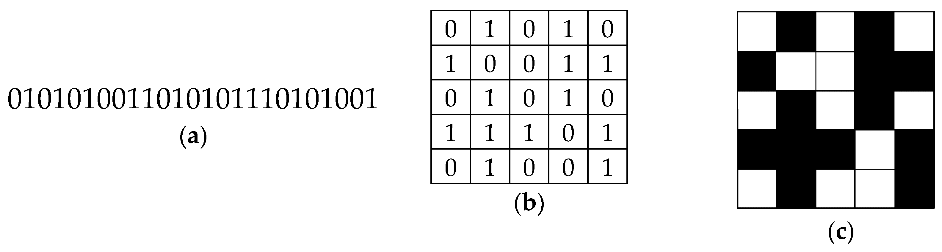
The design domain of the two-dimensional continuous structure is discretized into small and square elements in the finite element model (FEM), where each element represents either a material or a void. The binary string or bit-array is used to store the design information. In the string, the code “0” refers to a void element, while the code “1” represents a solid element in FEM. In this study, the stiffness of the void element is considered $k_{void}={10}^{-9}{k}_{solid}$ instead of zero stiffness to avoid the singularity of the global stiffness matrix in FEM. The decoding step of the binary string into a two-dimensional design domain (topology design) is simple, as shown in Figure 1. In particular, for a 5 × 5 design problem, a binary string of 25 bits is generated (Figure 1a). Then, a 5 × 5 matrix is organized as follows: the first five bits construct the first row, the bits from 6 to 10 contract the second row, and so on (Figure 1b). Finally, the code “0” is replaced by a void element, while the code “1” is replaced by a solid element (Figure 1c). If a matrix has $m$ rows and $n$ columns, the mathematical expression to map a string into a matrix is as follows:

$$k=0,1,\dots ,n.m-1$$

(19)

$$i=k\mathit{d}\mathit{i}\mathit{v}n$$

(20)

$$j=k\mathit{m}\mathit{o}\mathit{d}n$$

(21)

$$i=0,1,\dots ,m-1\mathrm{and}j=0,1,\dots ,n-1$$

(22)

where $k$ represents the location of the element in the binary string, $\mathit{d}\mathit{i}\mathit{v}$ is the integer division operation, and $\mathit{m}\mathit{o}\mathit{d}$ is modulo division operation.

During the optimization process, the BBA generates binary strings (designs) to be evaluated. These designs are mapped to the topology designs as described in the previous paragraph. Then, FE analyses are carried out to calculate each design’s compliance to find the associated penalty function value (Equation (8)). The current iteration penalty function values are used to find the best design of the current iteration and to generate the next iteration designs (as briefly described in Section 3).

This presentation method does not prevent the formation of the following issues (Wang and Tai [4]):

• Disconnected structures. This happens when one or a group of solid elements are surrounded by voids elements.
• Checkerboard patterns. It occurs when one or more solid elements are not adjacent to any other solid elements, but they are connected to other solid elements by their corners. For example, as shown in Figure 1c, the element in the first row and the second column are connected to the element in the second row and first column by their corners, but both are not adjacent to other solid elements.
• Many scattered void elements. These types of elements prevent the optimization algorithm from converging to good designs; moreover, such configurations would be difficult to manufacture. Figure 2a shows the first design example topology at iteration 1000. Here, there are too many scattered void elements. This issue, which was observed in fine finite element meshes, is addressed and solved in this study.
• Solid elements that share one edge with the continuous structure (see Figure 2a). It was observed that these types of elements will eventually be eliminated because they do not reduce the compliance while increasing the volume. This issue is addressed and solved in this study.

Design connectivity must be handled properly in the structural topology design to ensure the success of the BBA. A connected structure is referred to as a group of solid elements, each of which shares at least two edges with its neighboring elements with the exception of support and load elements that can share one edge with neighboring elements. Because of the four issues described above, it was necessary to develop an algorithm to modify the BBA designs before FE analysis. The proposed algorithm is based on the algorithm developed by Wu and Tseng [3], and new steps were added to suit the BBA and improve its convergence rate. The algorithm is stated as follows:

• Elements where supports or loads should be selected as the starting elements since these elements must exist. Code “2” is assigned to the staring elements. Now elements with supports and loads have the code “2” and the rest of the elements have either the code “0” or “1”.
• If an element with the code “1” shares an edge with an element with the code “2”, the code “1” is changed into the code “2”. This procedure is repeated until no element with the code “1” can be changed into the code “2”.
• Elements with the code “2” represent a continuous structure, and elements with the code “1” represent a discontinuous structure(s). The code “1” is changed into the code “0” while the code “2” is changed into the code “1”. In this way, the binary string representation of the structure topology is restored.
• If an element with the code “0” shares no edge with another element with the code “0” (i.e., void element surrounded by solid element), its code is changed into the code “1”.
• If an element with the code “1” is adjacent to only one element with the code “1” (i.e., solid element adjacent to three void elements), its code is changed into the code “0”.
• Finally, after steps 1 to 5 are applied, the modified design replaces the original design before step 1. It was observed that this step improved the convergence behavior of the algorithm because in the next iteration, the BBA tried to improve designs without isolated objects, many scattered void elements, and solid elements that shared one edge with the continuous structure. Moreover, few iterations of modification were needed (steps 1–5) in the next iteration designs because the modification of any new design occurred where there were new isolated objects, scattered void elements, and solid elements that shared one edge with the continuous structure. This step sped up the algorithm because few iterations of modification were needed.
• The initial design population (a matrix of all designs) must have one vector of ones. This design is a solid structure with no voids. The rest of the designs are generated randomly.

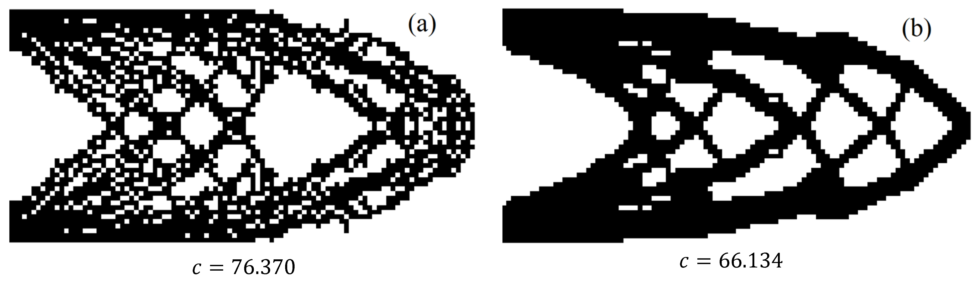
Steps 1 to 3 solved the discontinuity problem (issue 1), step 4 solved the checkerboard and scattered void elements problems (issues 2 and 3), and step 5 solved issue 4. Figure 2 shows that steps 4 and 5 were necessary to improve the quality of the topology designs. That is, for the first design example, at iteration 1000, the compliance was reduced by about $13.4\%$ (there was no volume violation in both cases) by adding steps 4 and 5 to the algorithm. Moreover, the design that is shown in Figure 2b is more practical in comparison with the design shown in Figure 2a.

5. Numerical Examples

Four benchmark structural topology optimization problems were employed to examine the search capability of the bit-array representation with the BBA and the proposed filtering algorithm and merit function (Equation (8)).

The structures were analyzed using the finite element (direct stiffness) method, and the algorithms were coded using MATLAB. The BBA algorithmic parameters were set as follows: population size is $25$, the maximum number of iterations ($maxIter$) $10,000$, loudness ($A$) is $0.75$, and pulse rate ($r$) is $0.01$. These parameters are selected depending on the problem. Thus, in this study, they are set based on the experience gained after some testing runs. The minimum and maximum pulse frequencies are 0 and 2, respectively.

Because the BBA is stochastic in nature, five independent optimization runs were performed for each example and the best topology is reported here. It is interesting to note that each independent run produced not only a different compliance but also different configuration because of the random search nature of metaheuristic algorithms.

In all problems, the objective was to find the minimum compliance subjected to a maximum volume constraint of $0.5$ (i.e., $Vo{l}_{solid}/Vol\le 50\%$), Young’s modulus is $1$ unit force/unit area, and Poisson’s ratio is $0.3$. For design examples 1, 2, 4, and 5, the design domain is rectangular of $2$ unit lengths in the $x$ direction and $1$ unit length in the $y$ direction. For the finite element analysis, the domain is divided into $100\times 50$ quadrilateral square plane stress elements. That is, the total number of design variables is $5000$ because each element is a design variable with 0 or 1 values. For design example 3, the design domain is rectangular of $3$ unit lengths in the $x$ direction and $1$ unit length in the $y$ direction. For the finite element analysis, the domain is divided into $150\times 50$ quadrilateral square plane stress elements (7500 elements). This mesh size is chosen because the SIMP method becomes less mesh-dependent when the mesh is fine. Although a finer mesh produces a slightly better design, it is more computationally expensive. The numerical results from the present bit-array representation with the BBA are compared with those from the SIMP method using Sigmund’s 99 line topology optimization code written in MATLAB [27]. In the power law approach, the penalization power and the filter size are set to 3 and 1.2, respectively.

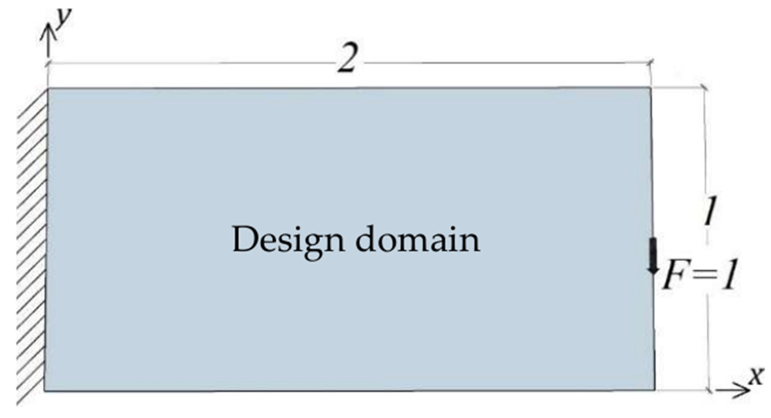
5.1. The Cantilever Plate Problem (Case 1)

The problem is illustrated in Figure 3, which shows a cantilever plate subjected to a point load. That is, the left boundary is fixed, and a unit point load is applied vertically downward at half the height of the right boundary. The problem was previously solved by Wu and Tseng [3] and Wang and Tai [4] using GA and a mesh size of $24\times 12$ ($288$ elements).

Table 1. Comparison of the best topologies of the cantilever plate (case 1).

Method	$\mathbf{Mesh}\mathbf{Size}:100\times 50$	$\mathbf{Compliance}\left(\mathit{c}\right)$
Solid Isotopic Microstructure with Penalization (SIMP)		$63.897$
Binary Bat Algorithm (BBA) without symmetry		$63.249$
BBA with symmetry		$62.162$

shows the topology designs obtained by the SIMP method, the BBA without symmetry (5000 design variables), and the BBA with symmetry (2500 design variables), as well as their corresponding compliances. The symmetry is taken around an axis parallel to the $x$-axis and passing through $0.5$ on the $y$-axis. Although the SIMP method with a mesh size of $100\times 50$ produced distinct boundaries, many gray elements were found due to the smoothing filtering across the edges. The mass density is taken as a continuous design variable rather than a discrete binary variable [3,4]. Using the SIMP method, the minimum compliance of $63.897$ is obtained at iteration 184. With a mesh size of $140\times 70$ (9800 elements), the minimum compliance of $63.2$ is obtained at iteration 557. However, the computation time increased about 33 times. This result shows that a mesh size of $100\times 50$ is resealable for the types of problems discussed in this study. Topology optimization using the present bit-array with the BBA is performed without and with symmetry. In both cases, it can be seen that the distinct black (material) and white (void) design topology are obtained because discrete binary design variables are employed. The minimum compliances of $63.249$ and $62.162$ are obtained from the BAA without symmetry and the BBA with symmetry, respectively. Minimum compliances of 64.44 and 65.26 were found by Wu and Tseng [3] and Wang and Tai [4] using GA, respectively. Therefore, better compliances were found using the present bit-array with BBA but with different configurations (see Table 1).

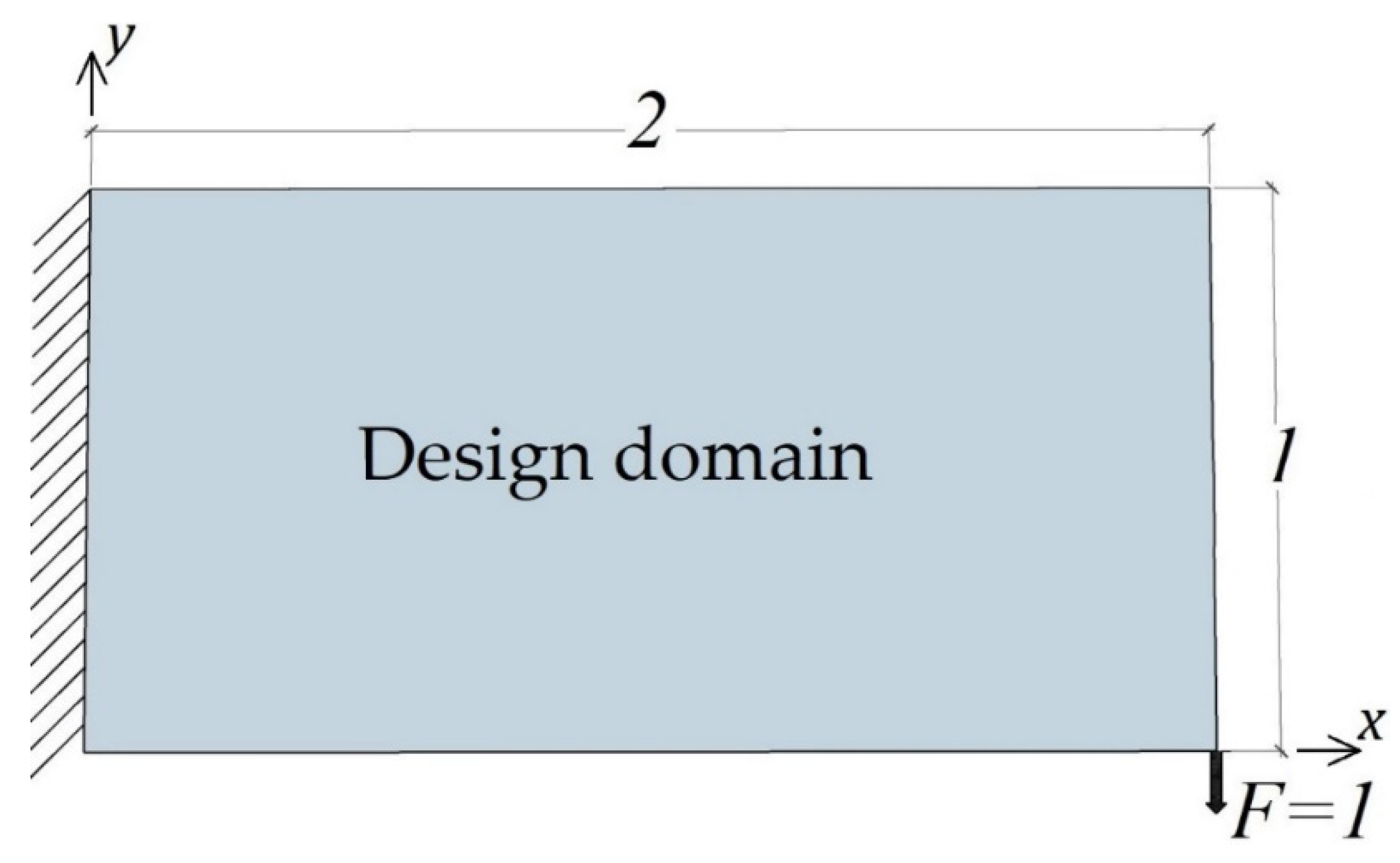
5.2. The Cantilever Plate Problem (Case 2)

The problem is illustrated in Figure 4. This problem is similar to the problem described in Section 5.1. However, the location of the point load is different. That is, the left boundary is fixed, and the unit point load is applied vertically downward at the bottom right corner. To the best of the authors’ knowledge, this problem has not been previously solved before using metaheuristic algorithms.

Table 2. Comparison of the best topologies of the cantilever plate (case 2).

Method	Mesh Size: 100 × 50	$\mathbf{Compliance}\left(\mathit{c}\right)$
SIMP		$70.877$
BBA without symmetry		$70.404$

shows the topology designs obtained by using the power law approach and the BBA without symmetry as well as their corresponding compliances. In this problem, symmetry is not applicable. Minimum compliances of $70.877$ and $70.404$ were obtained using the SIMP method and the bit-array with the BBA, respectively. The present bit-array with the BBA resulted in slightly less compliance than the SIMP method did but there were no blurry boundaries.

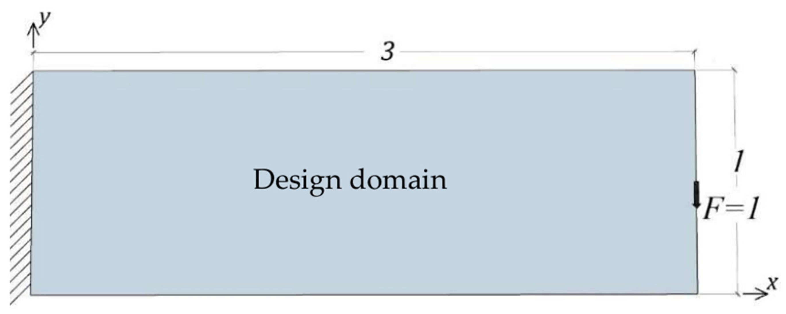
5.3. The Cantliver Plate Problem (Case 3)

The third example is the $3\times 1$ cantilever beam. Figure 5 demonstrates the problem definition. This problem is similar to the first design example (Section 5.1). However, in this case, the beam is one unit-length longer. The problem was previously solved by Gao [10] using the CDT method with a mesh size of $150\times 50$ ($7500$ elements).

Table 3. Comparison of the best topologies of the cantilever plate (case 3).

Method	$\mathbf{Mesh}\mathbf{Size}:150\times 50$	$\mathbf{Compliance}\left(\mathit{c}\right)$
BBA with symmetry		$177.730$

shows the final design layout and compliance of the BBA with symmetry. The proposed bit-array with BBA converged to compliance of 177.73 where the CDT and the SIMP methods reached minimum compliances of 182.475 and 182.816, respectively [10]. The presented result in this study shows no checkerboard patterns or grayscale areas as in those from the CDT and the SIMP methods.

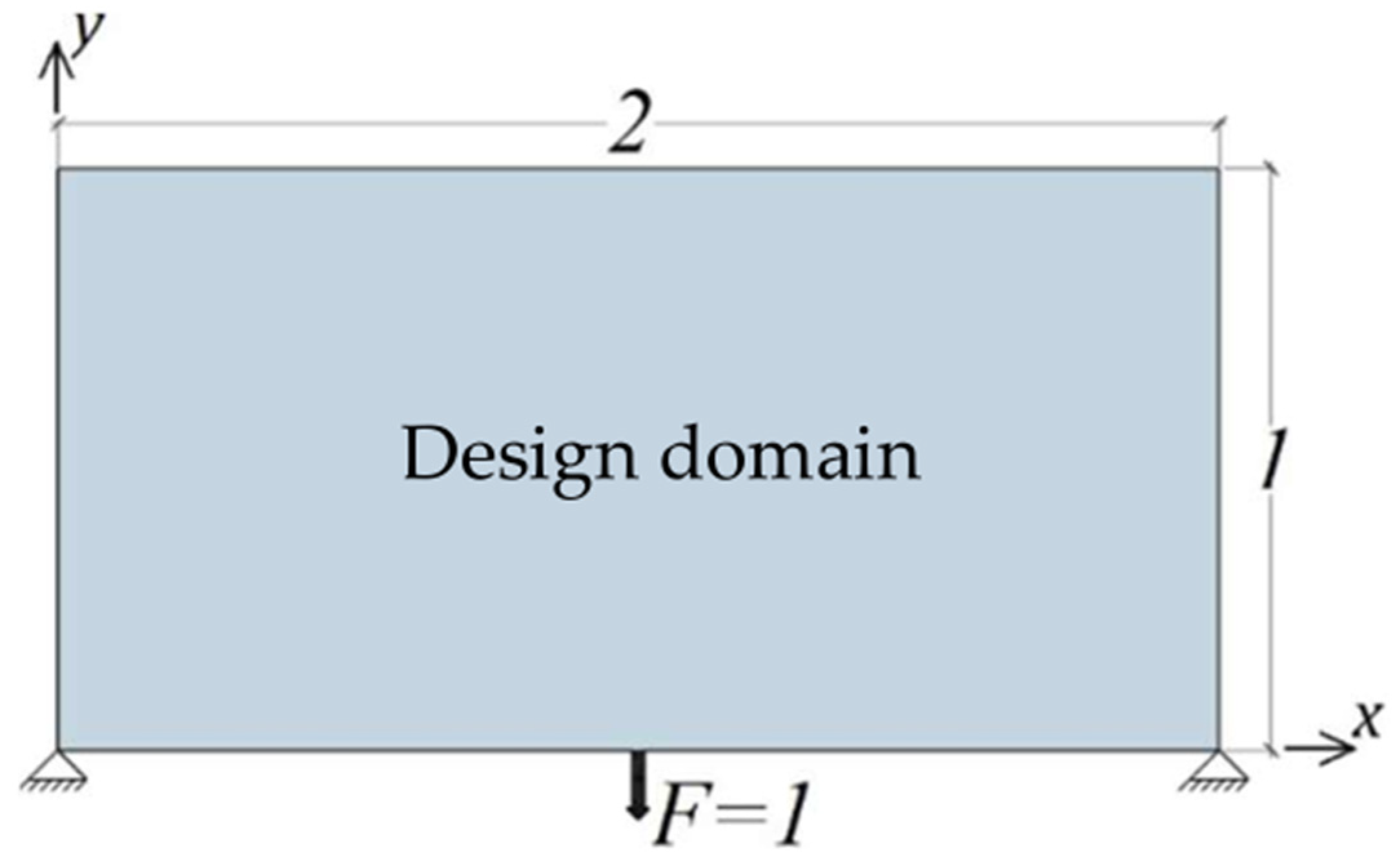
5.4. The Pined-Pined Plate Problem

The problem definition is illustrated in Figure 6. The nodes at the left and right bottom are set as fixed nodal displacements, and the unit point load is applied vertically downward at half the length of the bottom boundary. This problem was previously solved by Kaveh et al. [33] using the Ant Colony algorithm with a mesh size of $80\times 40$ ($3200$ elements). However, the compliance of the final design was not provided.

The results derived by the SIMP method, the BBA without symmetry, and the BBA with symmetry as well as their corresponding minimum compliances are shown in

Table 4. Comparison of the best topologies of the pinned-pined plate.

Method	Mesh Size: 100 × 50	$\mathbf{Compliance}\left(\mathit{c}\right)$
SIMP		$9.951$
BBA without symmetry		$9.811$
BBA with symmetry		$9.797$

. The symmetry is taken around the axis parallel to the $y$-axis passing through $1$ on the $x$-axis. Table 4 demonstrates that the proposed bit-array with the BBA converges to better solutions.

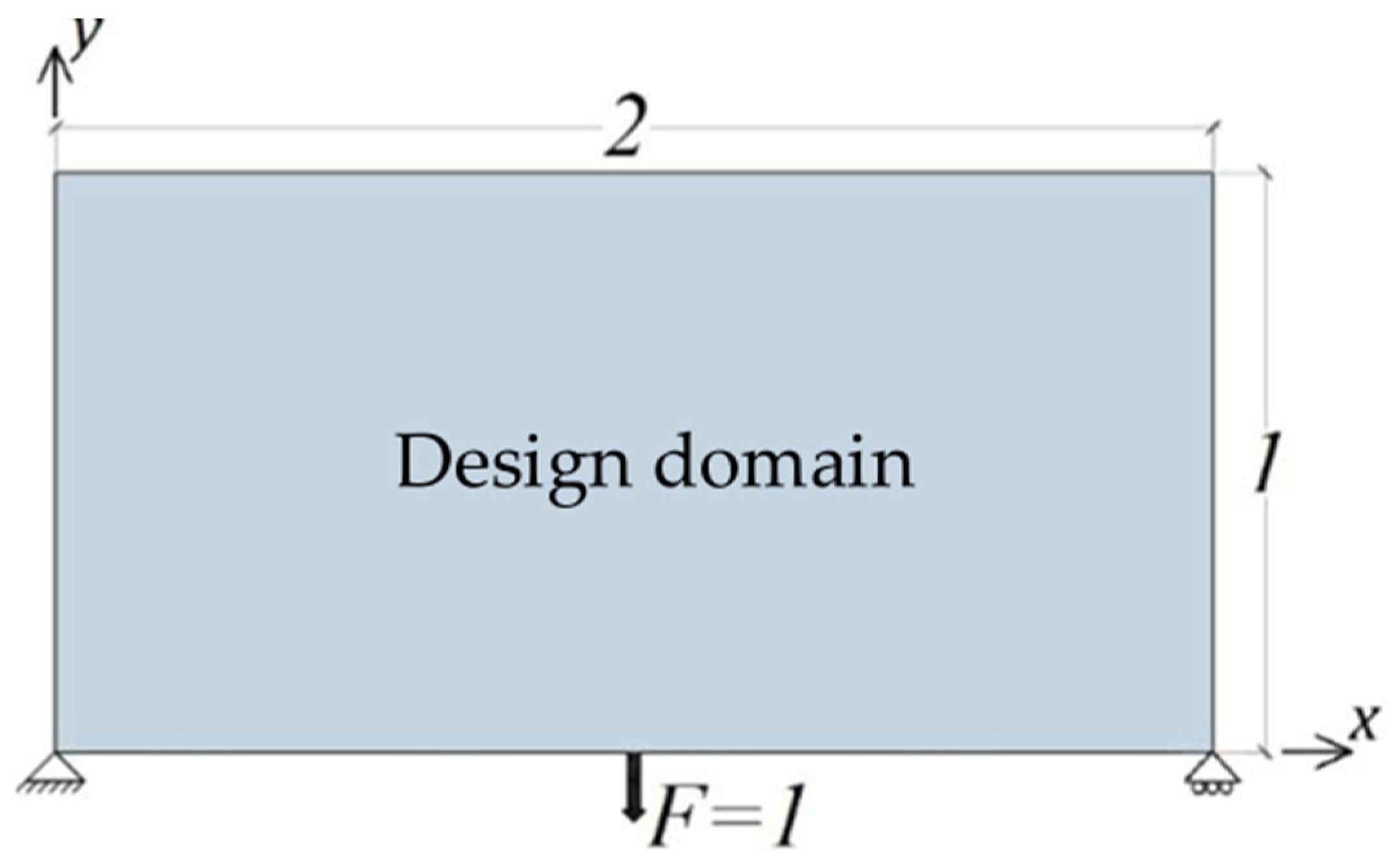
5.5. The Pined-Roller Plate Problem

The problem definition is illustrated in Figure 7. This problem is similar to the problem in Section 5.3. However, the pinned support on the right side is replaced by a roller support. A unit point load is applied vertically downward at the half-length of the bottom boundary. This problem was previously solved by Kaveh et al. [33] using the Ant Colony algorithm with a mesh size of ($3200$ elements). However, the compliance of the final design was not provided.

Table 5. Comparison of the best topologies of the pinned-roller plate.

Method	Mesh Size: 100 × 50	$\mathbf{Compliance}\left(\mathit{c}\right)$
SIMP		$14.460$
BBA without symmetry		$14.450$
BBA with symmetry		$14.326$

shows the layouts obtained after the optimization process and the minimum compliances of the SIMP method, the BBA without symmetry, and the BBA with symmetry. The symmetry is taken around the axis parallel to the $y$-axis passing through $1$ on the $x$-axis. Again, the minimum compliances of the proposed bit-array representation are slightly better the SIMP method but with no blurry boundaries and the final design configurations are different.

According to the results discussed in Section 5.1, Section 5.4, and Section 5.5, the BBA with symmetry is the best among the three methods because the number of design variables in the symmetrical problems is reduced to half. Therefore, the number of possible combinations is also reduced to half.

6. Conclusions

In topology structural optimization, it is desirable to obtain designs without greyscale areas, which requires using discrete design variables with void or material elements after discretizing the design domain by using a finite element mesh.

In this study, a bit-array (0/1) representation method for structural topology optimization using the binary bat algorithm (BBA) was implemented. A new filtering algorithm and penalty function were incorporated with the BBA to avoid the formation of isolated elements and checkerboard patterns as well as to improve the convergence rate toward the minimum compliance. The main advantage of the proposed algorithm is its ability to handle many design variables with no blurry areas. The numerical results of four well-known topology optimization problems with a mesh size of $100\times 50$ ($5000$ elements) and $150\times 50$ ($7500$ elements) showed that the proposed algorithm found better designs than the SIMP method but had a higher computational cost because of the global search nature of the metaheuristic algorithm. Thus, the proposed bit-array topology optimization algorithm appears to be very effective in solving large-scale topology optimization problems.

It is recommended that in future studies, the algorithm presented in this study should be applied to three-dimensional structural topology optimization problems.