Experiment on Interaction of Abutment, Steel H-Pile and Soil in Integral Abutment Jointless Bridges (IAJBs) under Low-Cycle Pseudo-Static Displacement Loads


 and
and 
Abstract
1. Introduction
2. Brief Introduction of Test
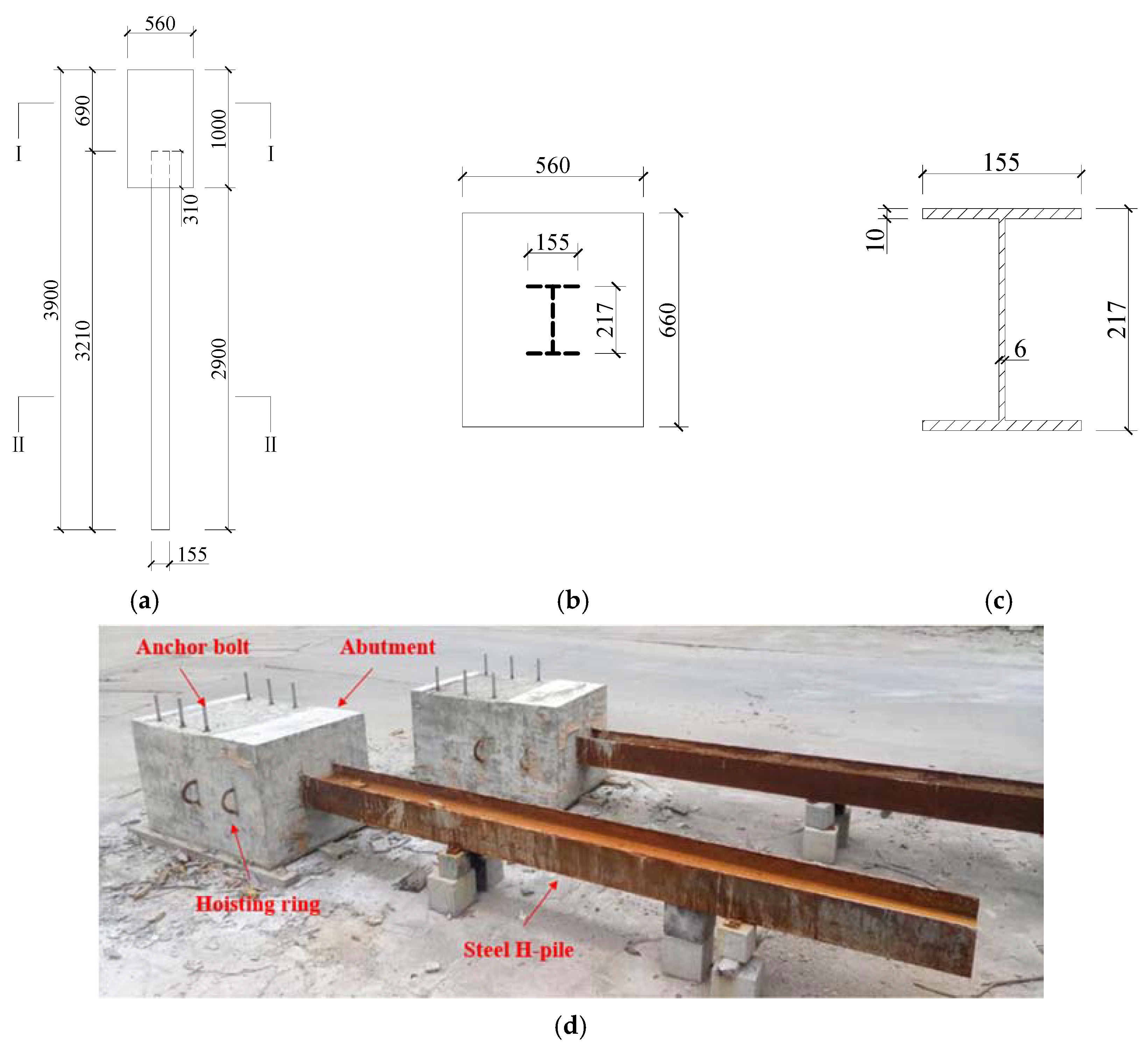
2.1. Specimen Design and Manufacturing
2.1.1. Specimen Design
2.1.2. Specimen Material and Soil Properties
Specimen Material Characteristics
Soil Properties
2.1.3. Specimen Manufacturing
2.2. Soil Box Design and Specimen Installation
2.2.1. Soil Box Design and Manufacturing
2.2.2. Specimen Orientation and Soil Filling
2.3. Layout of Measurement Points
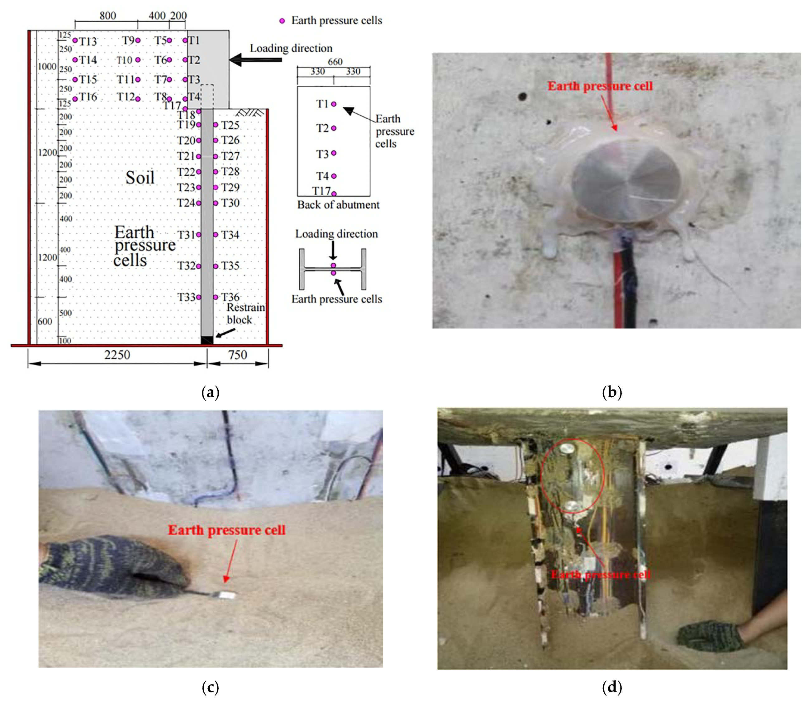
2.3.1. Layout of Earth Pressure Cells
2.3.2. Layout of Displacement Gages and Inclinometers
2.4. Loading Test
2.4.1. Loads
Horizontal Displacement loads
Vertical Weight
2.4.2. Loading Scheme
3. Experimental Results and Analyses
3.1. Earth Pressure behind Abutment
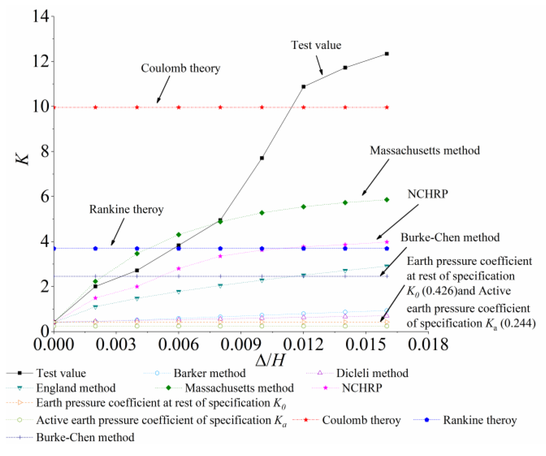
3.1.1. Relationship between Earth Pressure and Displacement Load
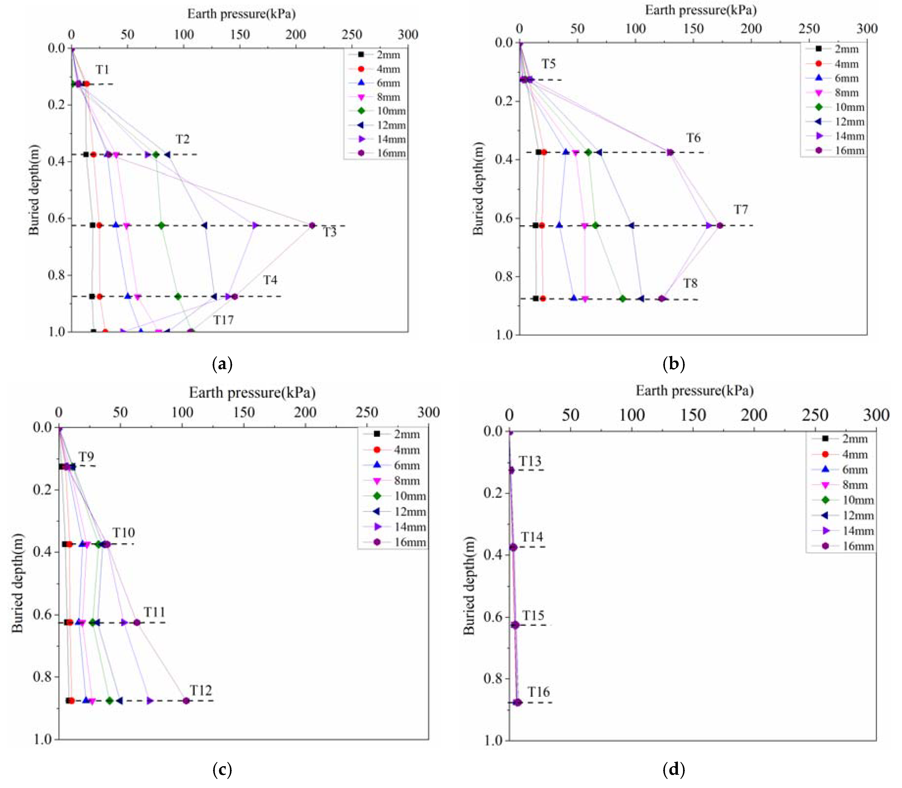
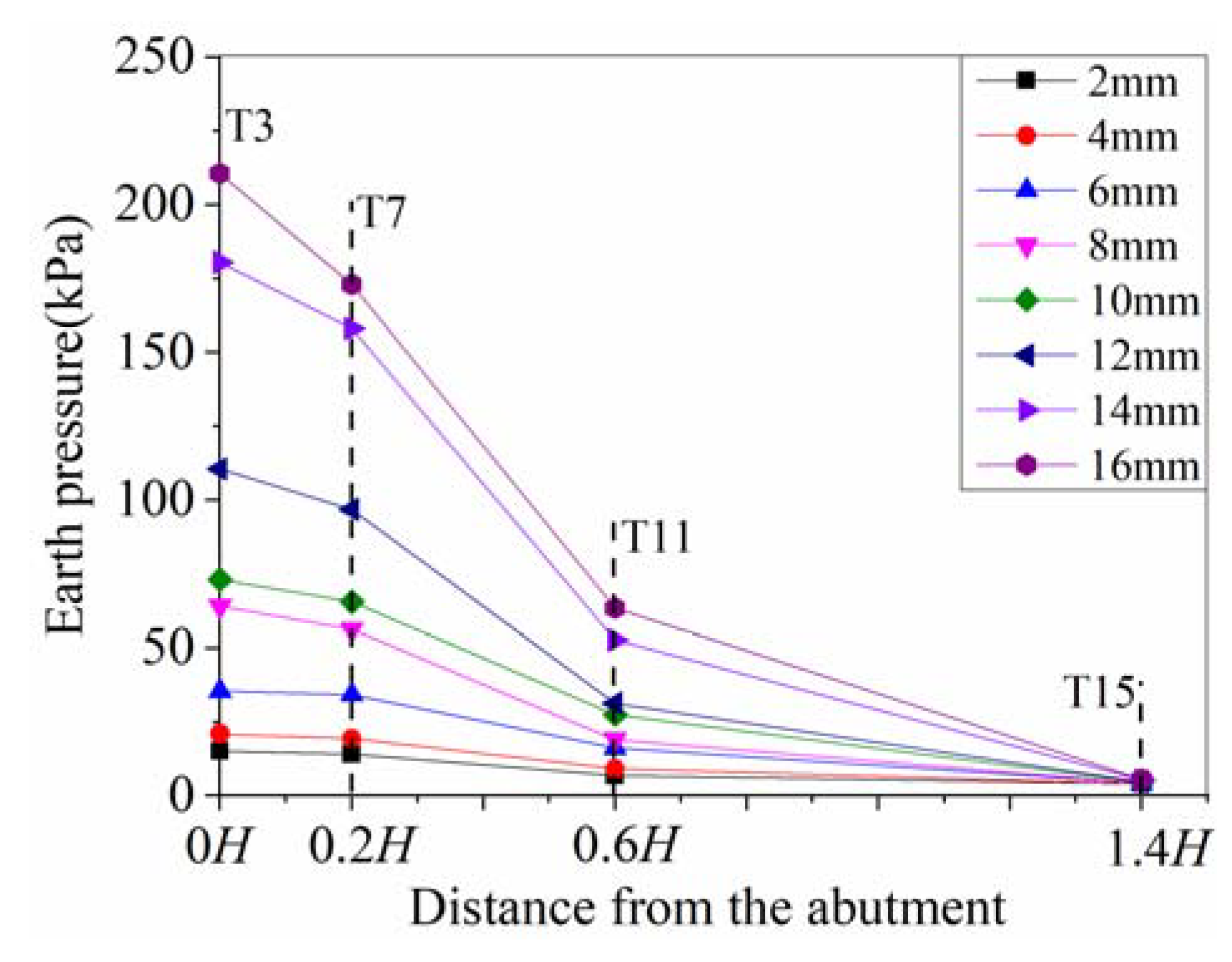
3.1.2. Distribution of Earth Pressure
Distribution along the Height of Abutment
Distribution along the Longitudinal Direction
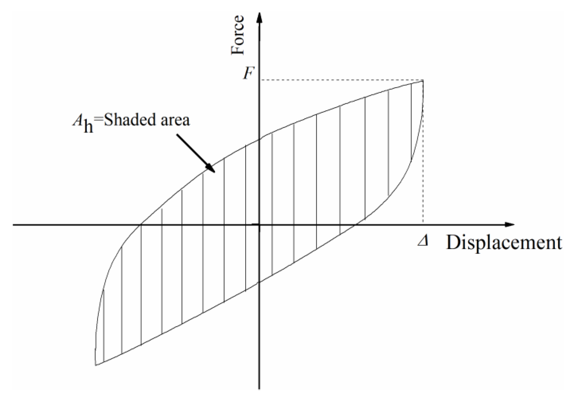
3.2. Hysteretic Curve and Skeleton Curve
3.2.1. Hysteretic Curve
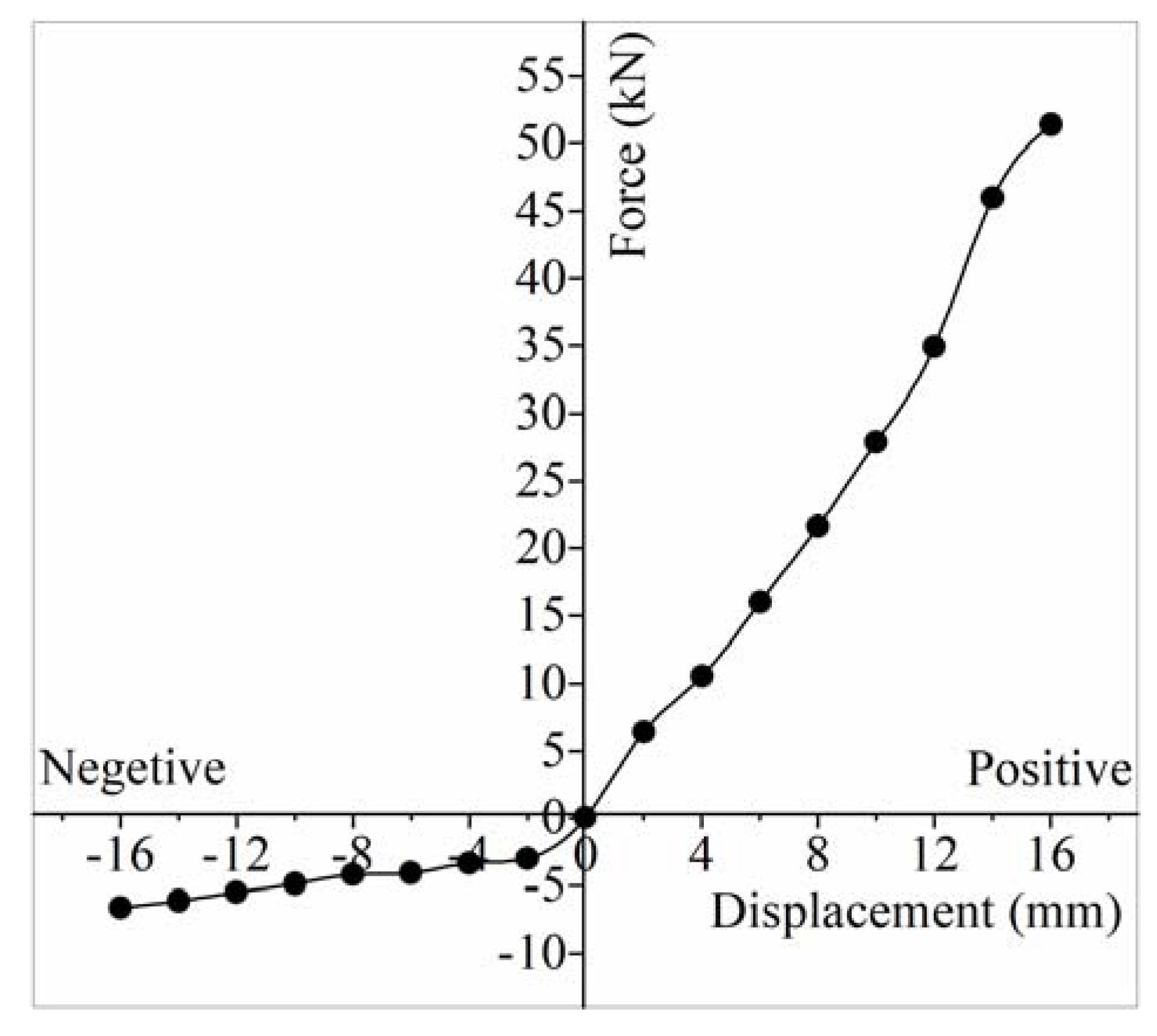
3.2.2. Skeleton Curve
3.3. Horizontal Deformation
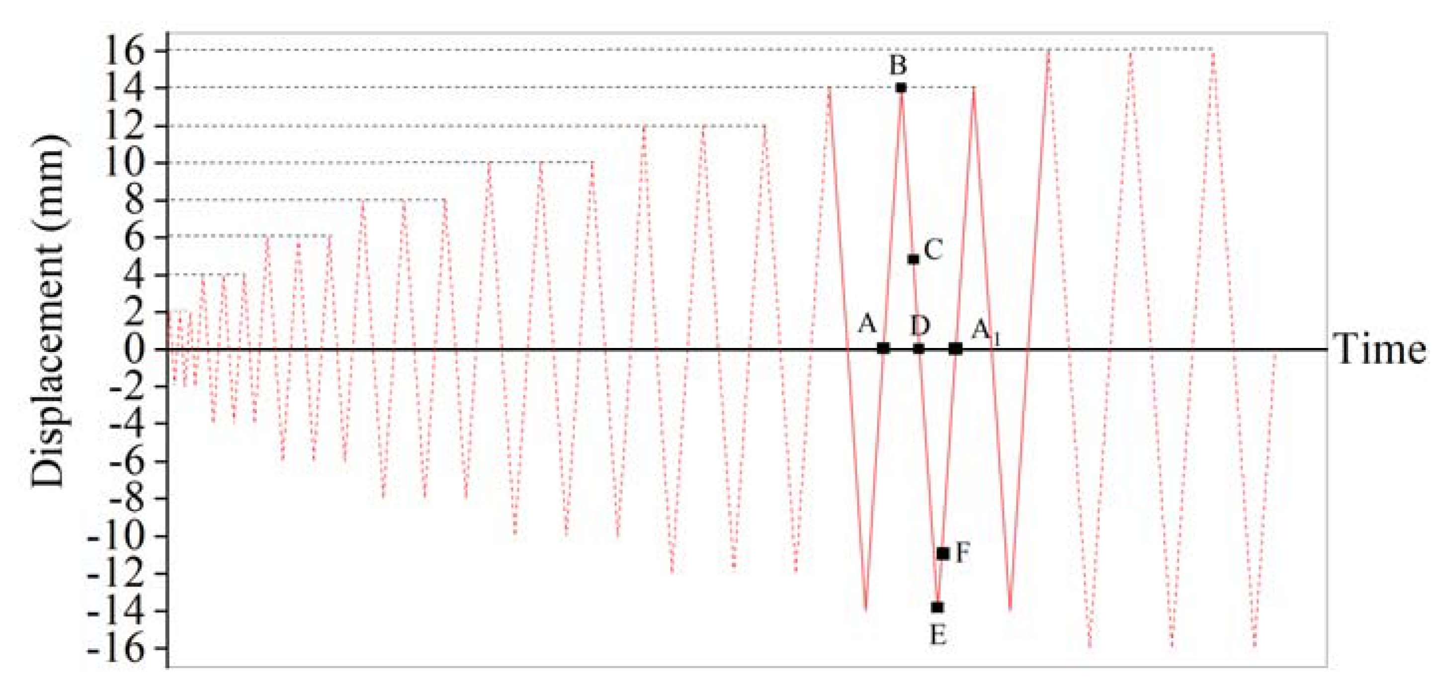
3.3.1. Time-History Curves of Horizontal Deformation
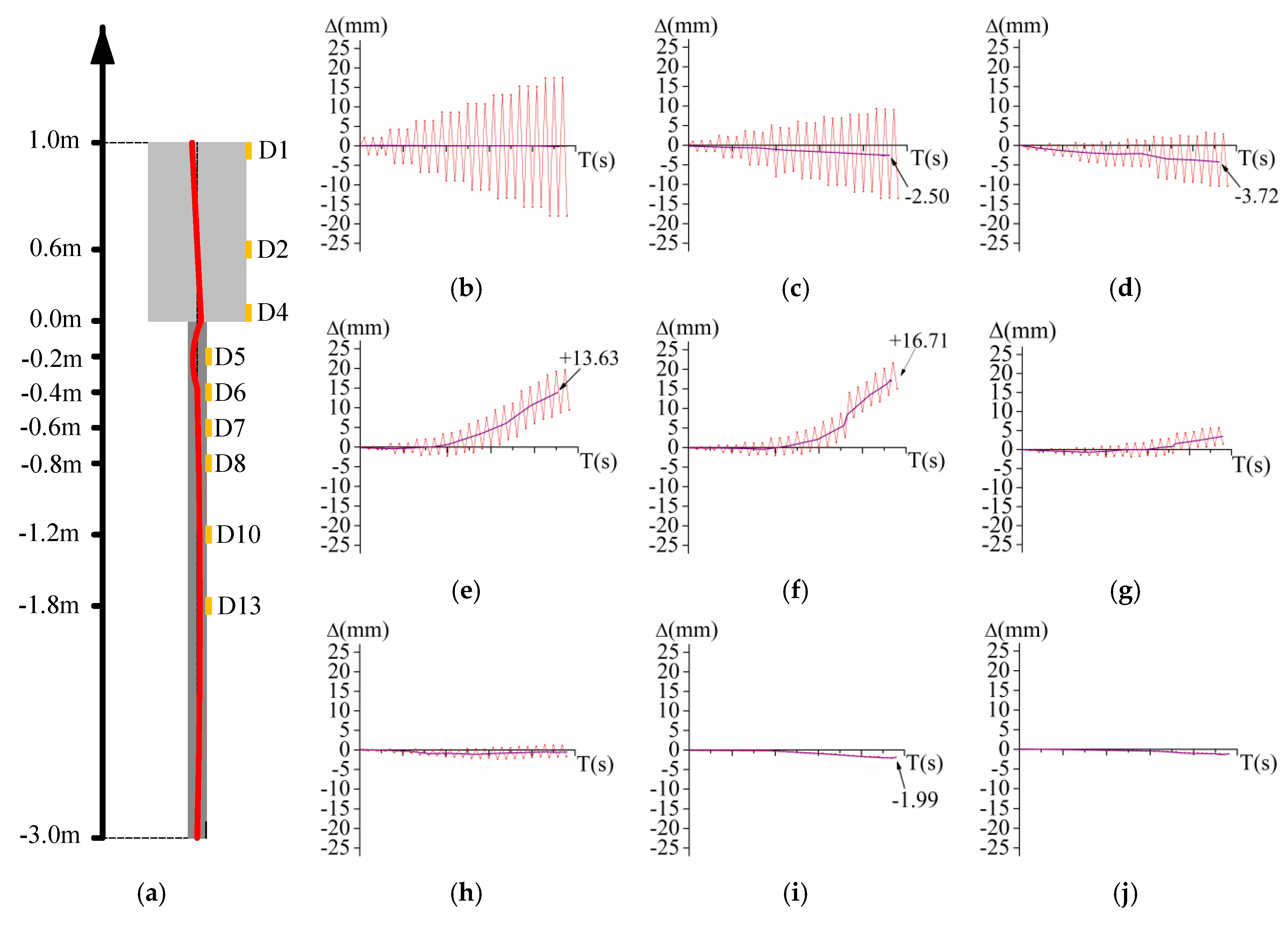
Time-History Curves Considering Accumulative Deformation
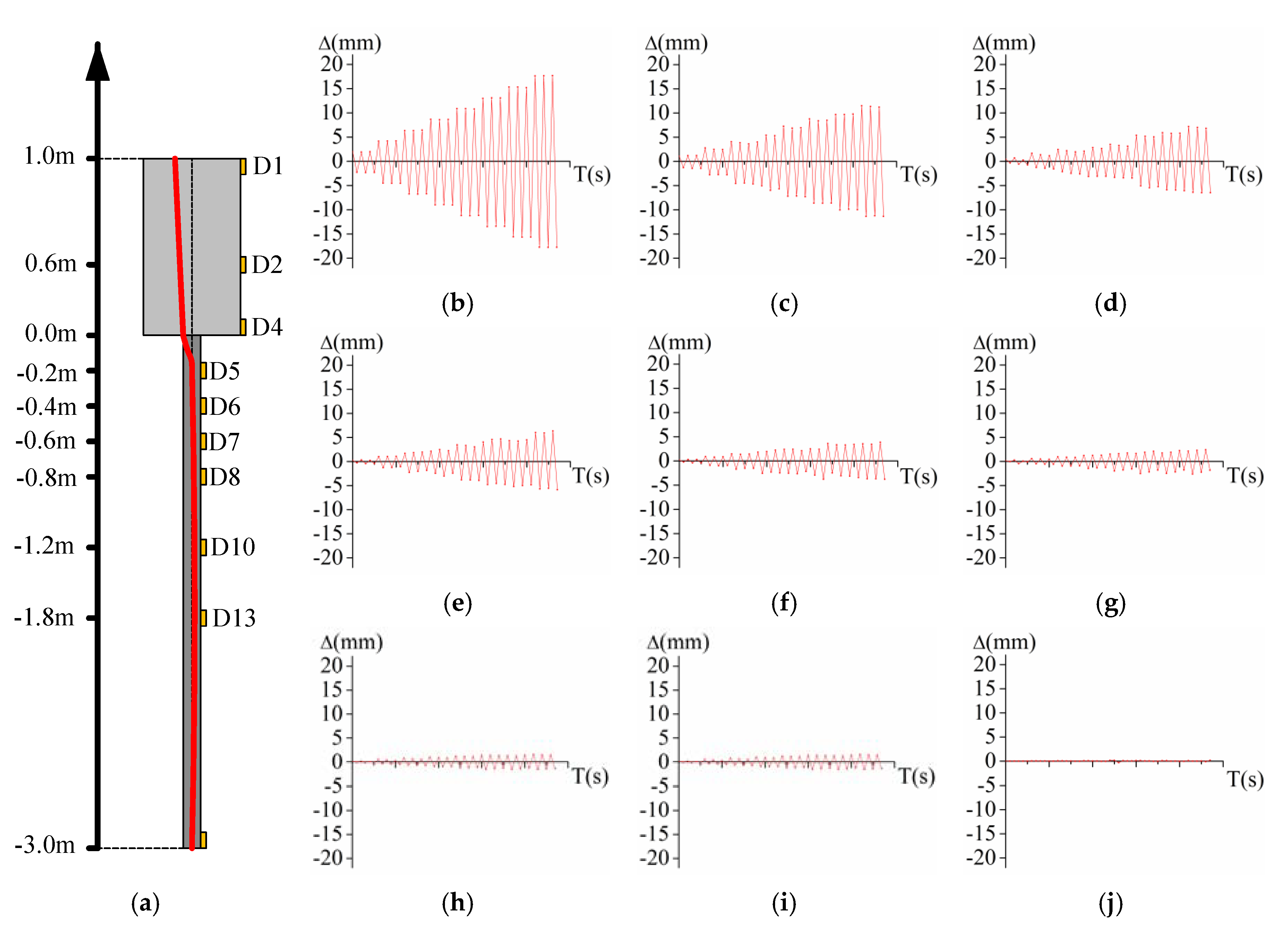
Time-History Curves Deducting Accumulative Deformation
3.3.2. Horizontal Deformation along the Depth
Horizontal Deformation under Positive Displacements
Horizontal Deformation under Negative Displacements
3.4. Rotation of Abutment
4. Conclusions
- (1)
- The passive earth pressure of backfill is over 30 times of active earth pressure, and the passive earth pressure coefficient is larger than those by others (Burke-Chen, Barker, NCHRP, Dicleli, England, Massachusetts, Rankine theory, Coulomb theory and JTG D60-2015) due to the ratcheting effect of soil. The existing calculation method earth pressure of backfill behind abutment is not accurate for that of IAJB.
- (2)
- The earth pressure behind abutment has a typical triangular distribution when the horizontal displacement is small (less than 8 mm), and it shows a trapezoid distribution when the soil is close to abutment under a large horizontal displacement (larger than 8 mm). The earth pressure at horizontal distances of 0.6H and 1.4H from the back of the abutment is triangular under different displacements. The pile has little influence on the distribution of earth pressure when distance exceeds 1.4H.
- (3)
- The accumulative deformation is observed and the hysteretic curves are dramatically asymmetrical, but the soil-abutment-pile system shows a linear behavior yet.
- (4)
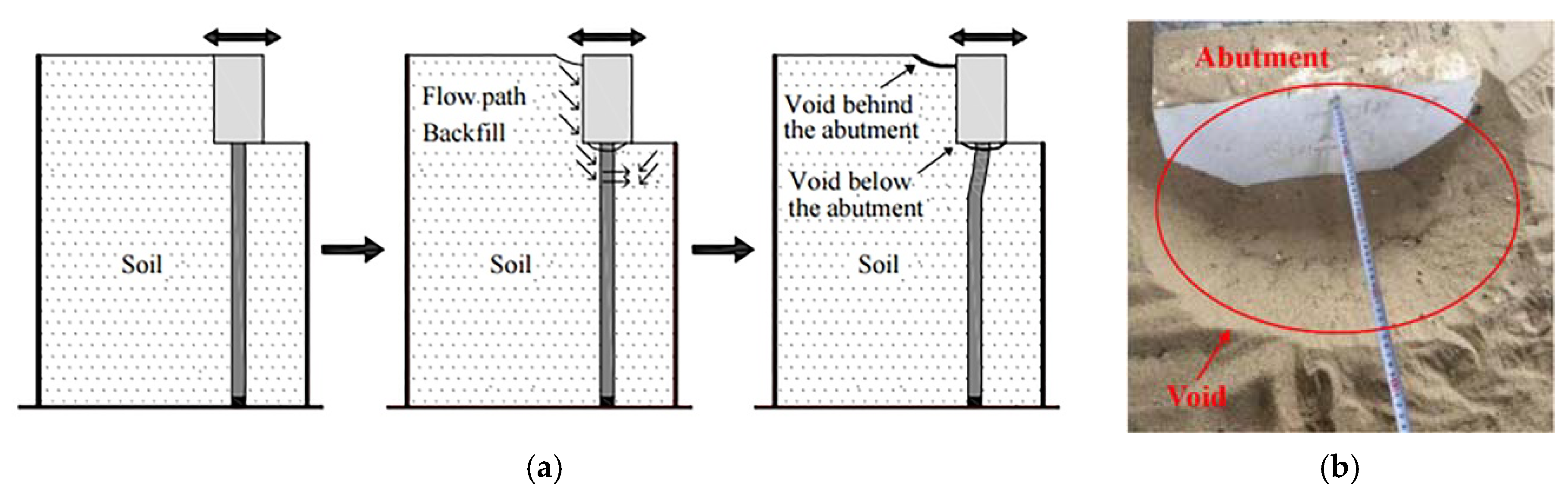
- The energy dissipation capacity when test specimen moves to the positive direction is much larger than that when specimen moves to the negative direction. The soil-abutment-pile system in IAJBs has favorable energy dissipation capacity and seismic behavior. The sum of horizontal deformation of abutment-pile-soil specimen are far larger than that of traditional pile-soil specimen due to the effect of accumulative deformation. Its maximum horizontal deformation occurs at the pile body rather than the pile head. The phenomenon of void is observed at the surface of the backfill and the interface between abutment and pile, which is also one of the reasons for bumping at bridge-end and settlement of soil.
- (5)
- The time-history horizontal accumulative deformation goes up with the increase of displacement load, and the growth rate becomes faster when the displacement load reaches 10 mm. The accumulative deformation is relatively small for the abutment, but it is large in the buried depth of 1.0b~3.0b for pile. The traditional calculated theory of deformation of pile is not appropriate to calculate the accumulative deformation. The noncumulative deformation is nearly the same as the deformation of traditional theory. The influence of accumulative deformation should be considered in practical engineering.
- (6)
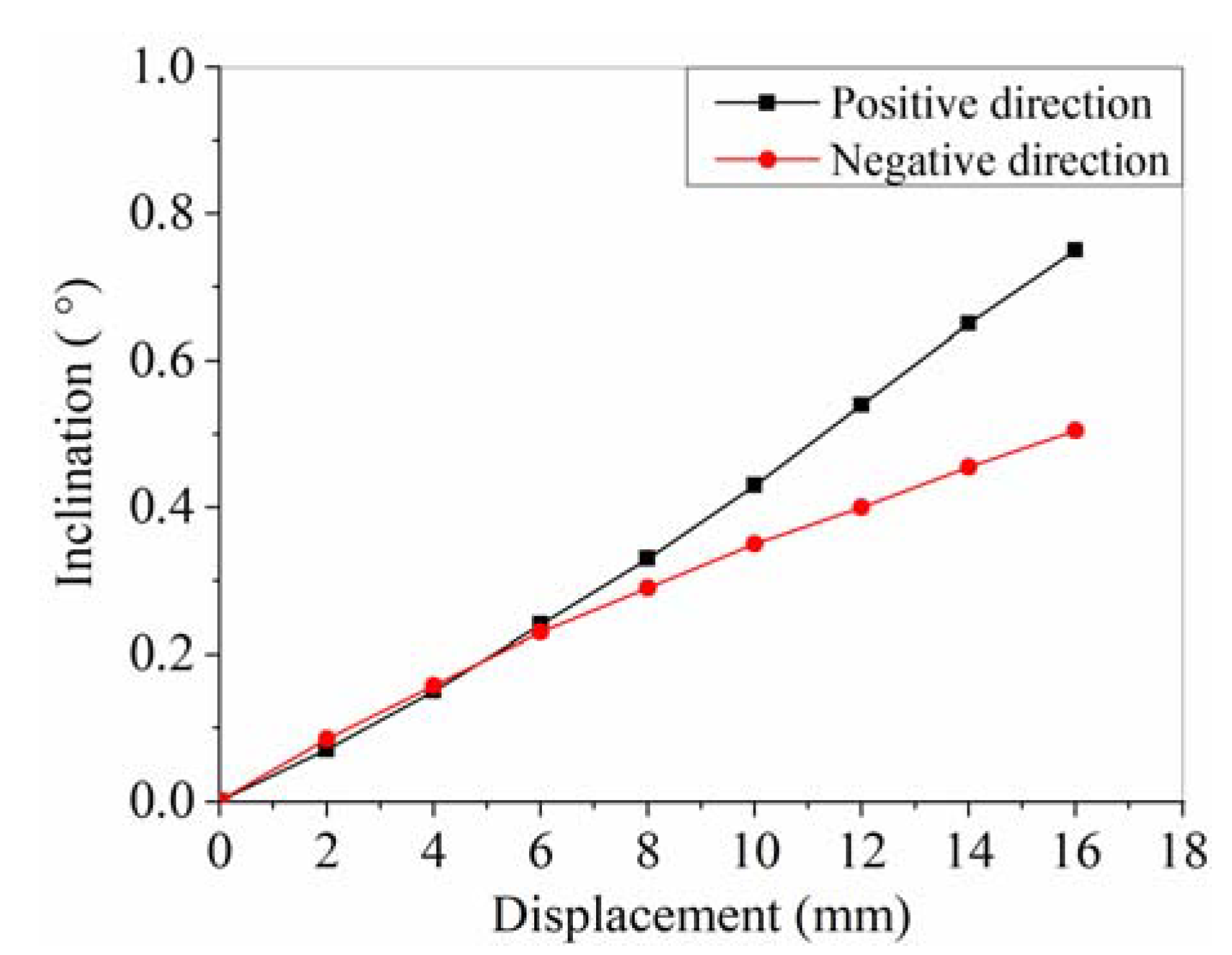
- A significant difference of inclinations in the positive and negative directions increases when the displacement load is relatively large. The rotation of abutment when bridge expands is larger than that when bridge contracts.
Author Contributions
Funding
Conflicts of Interest
References
- Kunin, J.; Alampalli, S. Integral Abutment Bridges: Current Practice in United States and Canada. J. Perform. Constr. Facil. 2000, 14, 104–111. [Google Scholar] [CrossRef]
- Frangi, A.; Collin, P.; Geier, R. Bridges with Integral Abutments: Introduction. Struct. Eng. Int. 2011, 21, 144. [Google Scholar] [CrossRef]
- White, H.; Pétursson, H.; Collin, P. Integral Abutment Bridges: The European Way. Pract. Period. Struct. Des. Constr. 2010, 15, 201–208. [Google Scholar] [CrossRef]
- Hassiotis, S.; Roman, E. A survey of current issues on the use of integral abutment bridges. Bridge Struct. 2005, 1, 81–101. [Google Scholar] [CrossRef]
- Jimin, H.; Carol, S.; Catherine, F. Behavior of an Integral Abutment Bridge in Minnesota, US. Struct. Eng. Int. 2011, 21, 320–331. [Google Scholar]
- Chen, B.C.; Zhuang, Y.Z.; Huang, F.Y.; Briseghella, B. Jointless Bridges, 2nd ed.; China Communication Press: Beijing, China, 2019. [Google Scholar]
- Guo, P.X.; Xiao, Y.; Kunnath, S.K. Performance of laterally loaded H-piles in sand. Soil Dyn. Earthq. Eng. 2014, 67, 316–325. [Google Scholar] [CrossRef]
- Huntley, S.A.; Valsangkar, A.J. Behaviour of H-piles supporting an integral abutment bridge. Can. Geotechnol. J. 2014, 51, 713–734. [Google Scholar] [CrossRef]
- Burdette, E.; Ingram, E.; Tidwell, J.; Goodpasture, D.; Deatherage, J.; Howard, S. Behavior of Integral Abutments Supported by Steel H-Piles. Transp. Res. Rec. J. Transp. Res. Board 2004, 1892, 24–28. [Google Scholar] [CrossRef]
- Luo, X.Y.; Huang, F.Y.; Zhuang, Y.Z.; Wu, S.W.; Qian, H.M. Modified Calculations of Lateral Displacement and Soil Pressure of Pile Considering Pile-Soil Interaction under Cyclic Loads. J. Test. Eval. 2019, 49. [Google Scholar] [CrossRef]
- Huang, J.; Shield, C.K.; French, C.E.W. Parametric Study of Concrete Integral Abutment Bridges. J. Bridge Eng. 2008, 13, 511–526. [Google Scholar] [CrossRef]
- Chen, Y.F. Important Considerations, Guidelines, and Practical Details of Integral Bridges. J. Eng. Technol. 1997, 14, 16–19. [Google Scholar]
- England, G.L.; Tsang, N.C.M.; Bush, D.I. Integral Bridges: A Fundamental Approach to the Time–Temperature Loading Problem; Thomas Telford: London, UK, 2000; pp. 151–152. [Google Scholar]
- Hong, J.X.; Peng, D.W.; Wang, X.H. Passive Earth Pressure Behind Abutment of Integral Abutment Bridges. J. Fuzhou Univ. (Nat. Sci.) 2003, 31, 721–725. (In Chinese) [Google Scholar]
- Peng, D.W.; Hong, J.X. Research on Simplified Calculating Model of Integral Abutment Bridges. Highway 2009, 54, 34–39. (In Chinese) [Google Scholar]
- Peng, D.W.; Chen, X.D.; Yuan, Y. Study on Seasonal Fluctuation of Earth Pressure Behind the Abutment. Chin. J. Geotechnol. Eng. 2003, 25, 135–139. (In Chinese) [Google Scholar]
- Yu, T.L.; Zhou, T.; Jiang, L.D.; Zhang, J.H. Study of Calculating Methods for Earth Pressure Behind Abutment of Integral Abutment Bridge Under Action of Rising Temperatures. Bridge Constr. 2010, 1, 29–35. (In Chinese) [Google Scholar]
- Janjic, D.; Bokan, H. Erection Control, TDV’s unique tool solution for bridge design and construction. IABSE Symp. Rep. 2006, 92, 97–104. [Google Scholar] [CrossRef]
- David, T.K.; Forth, J.P. Implementation of linear numerical analysis for integral abutment bridge-soil interaction. IEEE Colloq. Humanit. Sci. Eng. 2011, 82–87. [Google Scholar] [CrossRef]
- Take, W.A.; Bolton, M.D. Seasonal ratcheting and softening in clay slopes, leading to first-time failure. Géotechnique 2011, 61, 757–769. [Google Scholar] [CrossRef]
- Frosch, R.J.; Kreger, M.E.; Talbot, A.M. Earthquake Resistance of Integral Abutment Bridges. Ph.D. Thesis, Purdue University, Purdue, Germany, 2009. [Google Scholar]
- Guo, C.; Fu, B.Y.; Yuan, H.; Gong, W.M. Application and Field Tests of Cap-Pile Combined Foundation with Reversed Construction. Chin. J. Geotechnol. Eng. 2016, 38, 2085–2092. (In Chinese) [Google Scholar]
- Test Method of Soils for Highway Engineering; JTG E40-2007; China Communications Press: Beijing, China, 2007.
- Kulhawy, F.H.; Phoon, K.K. On the Evolution from Deterministic to Reliability-Based Foundation Design; Thomas Telford: London, UK, 2003; pp. 27–36. [Google Scholar]
- Zhao, M.H.; Xiao, Y.; Chen, C.F.; He, W. Analysis of Deformation on Soft Subsoil Around Bridge Abutment Considering Soil Creep Property. China J. Highw. Transp. 2006, 19, 56–61. (In Chinese) [Google Scholar]
- Huang, F.Y.; Wu, S.W.; Luo, X.Y.; Chen, B.C.; Lin, Y.W. Pseudo-static low cycle test on the mechanical behavior of PHC pipe piles with consideration of soil-pile interaction. Eng. Struct. 2018, 171, 992–1006. [Google Scholar] [CrossRef]
- Lou, M.L.; Wang, W.J.; Zhu, T.; Mang, H.C. Soil lateral boundary effect in shaking table model test of soil-structure system. Earthq. Eng. Eng. Dyn. 2000, 20, 30–36. [Google Scholar]
- Burke, J.R.; Martin, P. Design of integral concrete bridges. Concr. Int. 1993, 15, 37–42. [Google Scholar]
- Barker, R.M.; Duncan, J.M.; Rojiani, K.B.; Ooi PS, K.; Tan, C.K.; Kim, S.G. Manuals for the Design of Bridge Foundations: Shallow Foundations, Driven Piles, Retaining Walls and Abutment, Drilled Shafts, Estimating Tolerable Movements, and Load Factor Design Specifications and Commentary; Transportation Research Board: Washington, DC, USA, 1991. [Google Scholar]
- Dicleli, M. A rational design approach for prestressed-concrete-girder integral bridges. Eng. Struct. 2000, 22, 230–245. [Google Scholar] [CrossRef]
- Helmut, E. Geotechnical aspects of the mass-highway guidelines for integral abutment Bridges. In Design of Integral Abutment Bridges, BSCE/ASCE Geotechnical and Structural Groups Seminar; Bentley College: Waltham, MA, USA, 1999; pp. 207–224. [Google Scholar]
- General Specifications for Design of Highway Bridges and Culverts; JTG D60-201; China Communications Press: Beijing, China, 2015.
- Dicleli, M.; Albhaisi, S.M. Performance of Abutment–Backfill System Under Thermal Variations in Integral Bridges Built on Clay. Eng. Struct. 2004, 26, 949–962. [Google Scholar] [CrossRef]
- England, G.L.; Dunstan, T.; Tsang, C.M. Ratcheting flow of granular materials. In Static and Dynamic Properties of Gravelly Soils; ASCE: Reston, VA, USA, 2014. [Google Scholar]
- Anagnostopoulos, S.A. Equivalent Viscous Damping for Modeling Inelastic Impacts in Earthquake Pounding Problems. Earthq. Eng. Struct. Dyn. 2010, 33, 897–902. [Google Scholar] [CrossRef]
- Wijesundara, K.K.; Nascimbene, R.; Sullivan, T.J. Equivalent viscous damping for steel concentrically braced frame structures. Bull. Earthq. Eng. 2011, 9, 1535–1558. [Google Scholar] [CrossRef]
- Huang, F.Y.; Qian, H.M.; Zhuang, Y.Z. Experimental Study on the Dynamic Response of PHC Pipe-Piles in Liquefiable Soil. J. Test. Eval. 2017, 45, 230–241. [Google Scholar] [CrossRef]
- Novak, M.; Nogami, T. Soil-pile interaction in horizontal vibration. Earthq. Eng. Struct. Dyn. 1977, 5, 263–281. [Google Scholar] [CrossRef]
- Allani, M.; Holeyman, A. Flexural analysis in dynamic pinned head pile testing. Geotechnol. Geol. Eng. 2014, 32, 59–70. [Google Scholar] [CrossRef]
- Makris, N.; Gazetas, G. Dynamic pile-soil-pile interaction. Part II: Lateral and seismic response. Earthq. Eng. Struct. Dyn. 2010, 21, 145–162. [Google Scholar] [CrossRef]


| Water Content ω (%) | Density ρ (g/cm3) | Void Ratio e | Cohesive Ratio c (KPa) | Internal Friction angle φ (°) | Cu | Poisson Ratio v |
|---|---|---|---|---|---|---|
| 1.3 | 1.50 | 0.80 | 0 | 35 | 3.15 | 0.3 |
© 2020 by the authors. Licensee MDPI, Basel, Switzerland. This article is an open access article distributed under the terms and conditions of the Creative Commons Attribution (CC BY) license (http://creativecommons.org/licenses/by/4.0/).
Share and Cite
Huang, F.; Shan, Y.; Chen, G.; Lin, Y.; Tabatabai, H.; Briseghella, B. Experiment on Interaction of Abutment, Steel H-Pile and Soil in Integral Abutment Jointless Bridges (IAJBs) under Low-Cycle Pseudo-Static Displacement Loads. Appl. Sci. 2020, 10, 1358. https://doi.org/10.3390/app10041358
Huang F, Shan Y, Chen G, Lin Y, Tabatabai H, Briseghella B. Experiment on Interaction of Abutment, Steel H-Pile and Soil in Integral Abutment Jointless Bridges (IAJBs) under Low-Cycle Pseudo-Static Displacement Loads. Applied Sciences. 2020; 10(4):1358. https://doi.org/10.3390/app10041358
Chicago/Turabian StyleHuang, Fuyun, Yulin Shan, Guodong Chen, Youwei Lin, Habib Tabatabai, and Bruno Briseghella. 2020. "Experiment on Interaction of Abutment, Steel H-Pile and Soil in Integral Abutment Jointless Bridges (IAJBs) under Low-Cycle Pseudo-Static Displacement Loads" Applied Sciences 10, no. 4: 1358. https://doi.org/10.3390/app10041358
APA StyleHuang, F., Shan, Y., Chen, G., Lin, Y., Tabatabai, H., & Briseghella, B. (2020). Experiment on Interaction of Abutment, Steel H-Pile and Soil in Integral Abutment Jointless Bridges (IAJBs) under Low-Cycle Pseudo-Static Displacement Loads. Applied Sciences, 10(4), 1358. https://doi.org/10.3390/app10041358