A Review of Fault Diagnosing Methods in Power Transmission Systems


Abstract
1. Introduction
2. Disclose the Valuable Information
2.1. Transformations
2.1.1. Wavelet Transform (WT)
2.1.2. Fourier Transform (FT)
2.1.3. S-Transform (ST)
2.2. Dimensionality Reduction
2.3. Modal Transformation
3. Fault Detection (FD)
4. Fault-Types Classification (FC)
4.1. Artificial Neural Network (ANN) Based FC
4.1.1. Feedforward Neural Network (FNN)
4.1.2. Radial basis Function Network (RBFN)
4.1.3. Probabilistic Neural Network (PNN)
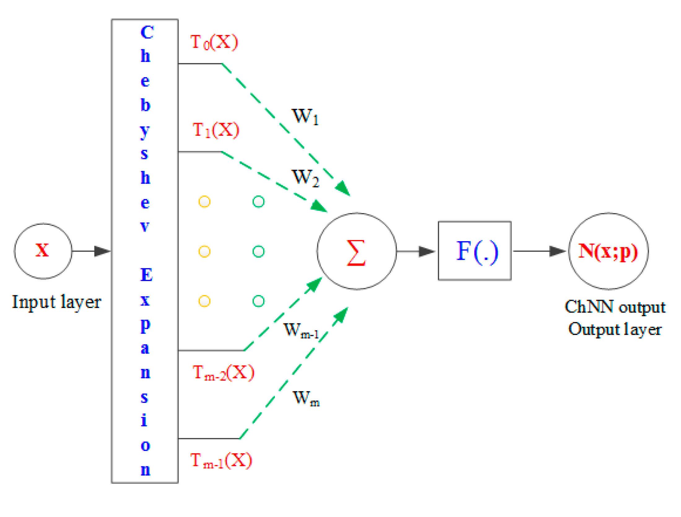
4.1.4. Chebyshev Neural Network (ChNN)
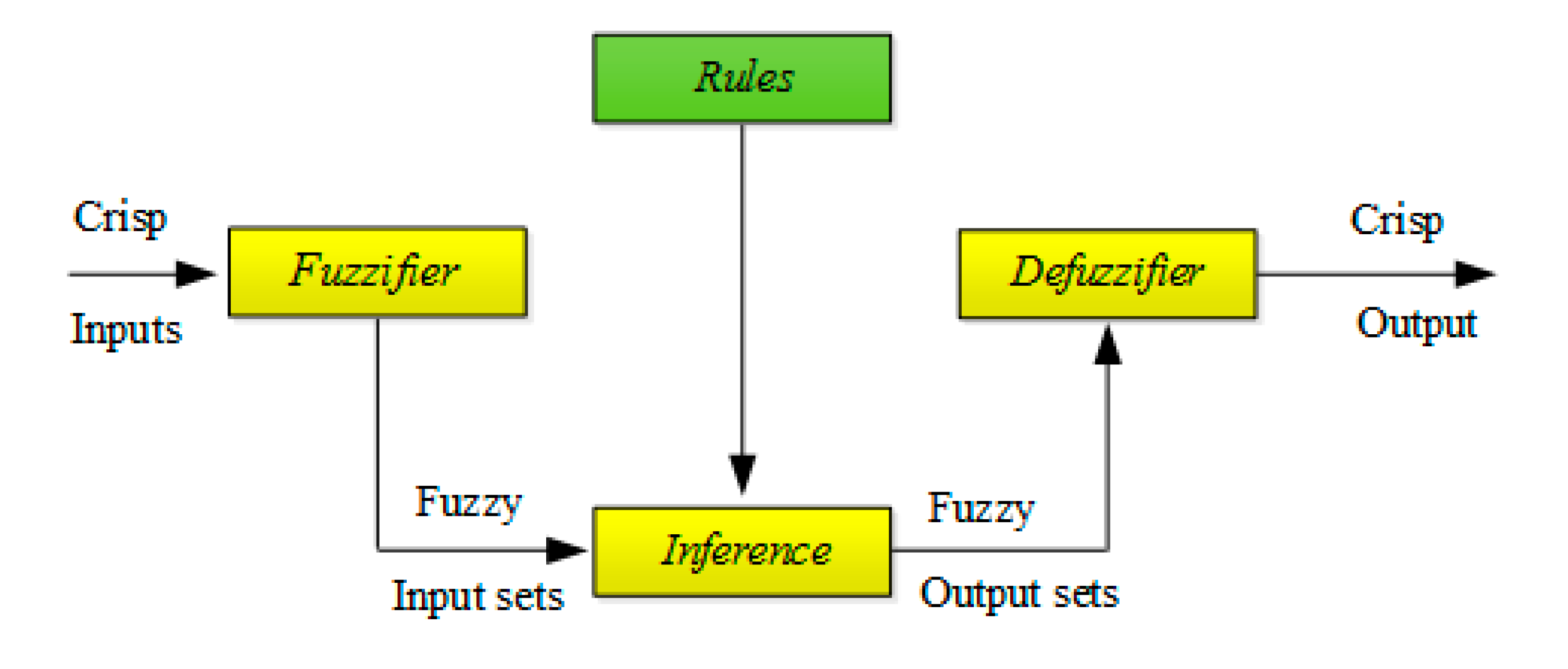
4.2. FC Based on Fuzzy Interface Systems (FIS)
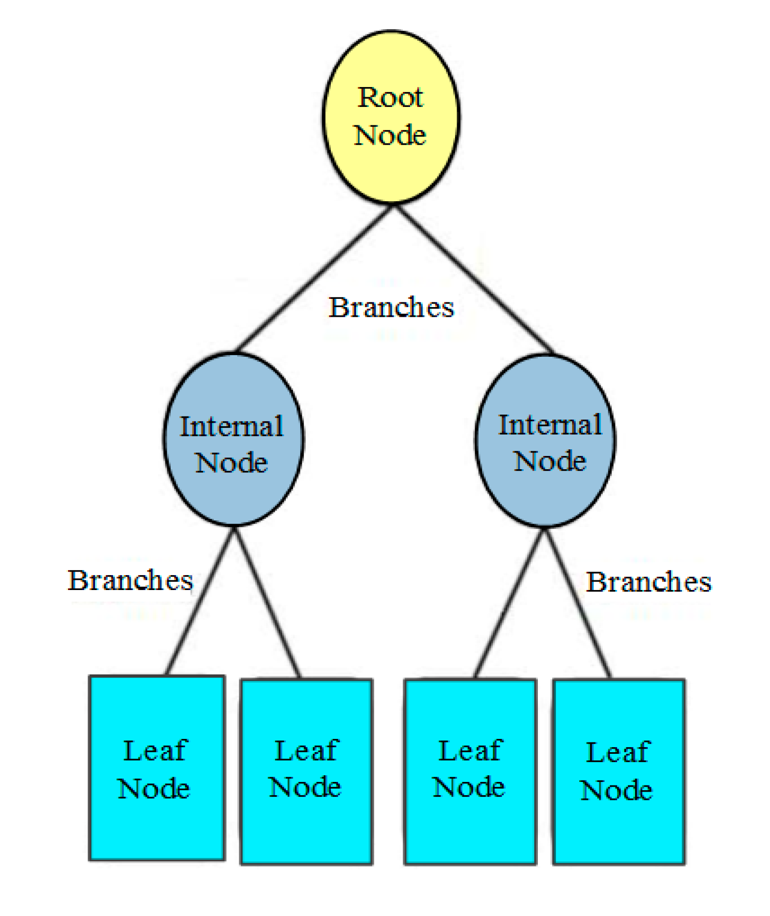
4.3. FC Based on Decision Tree (DT) Technique
4.4. FC Based on Support Vector Machine (SVM)
4.5. FC Based on Logic Flow (LF)
5. Comparison of Fault-Type Classification Methods
6. Future Trends in Fault-Type Classification
7. Fault Location Finding Methods
7.1. Wide-Area FL Approach
7.2. Fault Location Finding Algorithm for Series Compensated TLs
7.3. FL Methods for Hybrid TLs
7.4. ANN-based Algorithm for FL
7.5. FIS based Algorithm for FL
7.6. Support Vector Regression-Based Approach for FL
8. Comparison of Fault Location Methods
9. Future Trends in Fault Location Estimation
10. Weaknesses and Strengths of Different Emerging Computational Intelligence Methods
11. Conclusions
Author Contributions
Funding
Acknowledgments
Conflicts of Interest
References
- Shukla, S.K.; Koley, E.; Ghosh, S. DC offset estimation-based fault detection in transmission line during power swing using ensemble of decision tree. IET Sci. Meas. Technol. 2019, 13, 212–222. [Google Scholar] [CrossRef]
- Saber, A.; Emam, A.; Elghazaly, H. A Backup Protection Technique for Three-Terminal Multisection Compound Transmission Lines. IEEE Trans. Smart Grid 2018, 9, 5653–5663. [Google Scholar] [CrossRef]
- Swetapadma, A.; Yadav, A. A Novel Decision Tree Regression-Based Fault Distance Estimation Scheme for Transmission Lines. IEEE Trans. Power Deliv. 2017, 32, 234–245. [Google Scholar] [CrossRef]
- Almeidaa, A.R.; Almeidaa, O.M.; Juniora, B.; Barretob, L.; Barros, A.K. ICA feature extraction for the location and classification of faults in high-voltage transmission lines. Electron. Power Syst. Res. 2017, 148, 254–263. [Google Scholar] [CrossRef]
- Camarillo-Peñaranda, J.R.; Ramos, G. Fault Classification and Voltage Sag Parameter Computation Using Voltage Ellipses. IEEE Trans. Ind. Appl. 2019, 55, 92–97. [Google Scholar] [CrossRef]
- Pignati, M.; Zanni, L.; Romano, P.; Cherkaoui, R.; Paolone, M. Fault detection and faulted line identification in active distribution networks using synchrophasors-based real-time state estimation. IEEE Trans. Power Deliv. 2017, 32, 381–392. [Google Scholar] [CrossRef]
- Chen, K.; Huang, C.; He, J. Fault detection, classification and location for transmission lines and distribution systems: A review on the methods. IET High Volt. 2016, 1, 1–9. [Google Scholar] [CrossRef]
- Kezunovic, M. Smart fault location for smart grids. IEEE Trans. Smart Grid 2011, 2, 11–22. [Google Scholar] [CrossRef]
- Ouyang, Y.; He, J.; Hu, J.; Wang, S.X. A current sensor based on the giant magnetoresistance effect: Design and potential smart grid applications. Sensors 2012, 12, 15520–15541. [Google Scholar] [CrossRef]
- Han, J.; Hu, J.; Yang, Y.; Wang, Z.; Wang, S.X.; He, J. A nonintrusive power supply design for self-powered sensor networks in the smart grid by scavenging energy from AC power line. IEEE Trans. Ind. Electron. 2015, 62, 4398–4407. [Google Scholar] [CrossRef]
- Paithankar, Y.G.; Bhide, S.R. Fundamentals of Power System Protection; Prentice-Hall: Upper Saddle River, NJ, USA, 2003. [Google Scholar]
- Bo, Z.Q.; Jiang, F.; Chen, Z.; Dong, X.Z.; Weller, G.; Redfern, M.A. Transient based protection for power transmission systems. In Proceedings of the 2000 IEEE Power Engineering Society Winter Meeting, Singapore, 23–27 January 2000; pp. 1832–1837. [Google Scholar]
- Mallat, S. A Wavelet Tour of Signal Processing; Academic Press: Cambridge, MA, USA, 1999. [Google Scholar]
- Gawali, N.U.; Hasabe, R.; Vaidya, A. A comparison of different mother wavelet for fault detection & classification of series compensated transmission line. Int. J. Innov. Res. Sci. Technol. 2015, 1, 57–63. [Google Scholar]
- Kashyap, K.H.; Shenoy, U.J. Classification of power system faults using wavelet transforms and probabilistic neural networks. In Proceedings of the 2003 International Symposium on Circuits and Systems (ISCAS), Bangkok, Thailand, 25–28 May 2003; pp. 423–426. [Google Scholar]
- Parikh, U.B.; Das, B.; Maheshwari, R.P. Combined wavelet-SVM technique for fault zone detection in a series compensated transmission line. IEEE Trans. Power Deliv. 2008, 23, 1789–1794. [Google Scholar] [CrossRef]
- Malathi, V.; Marimuthu, N.S.; Baskar, S. Intelligent approaches using support vector machine and extreme learning machine for transmission line protection. Neurocomputing 2010, 73, 2160–2167. [Google Scholar] [CrossRef]
- Chanda, D.; Kishore, N.K.; Sinha, A.K. A wavelet multiresolution analysis for location of faults on transmission lines. Int. J. Electron. Power Energy Syst. 2003, 25, 59–69. [Google Scholar] [CrossRef]
- Jayabharata, R.; Mohanta, D.K. A wavelet-fuzzy combined approach for classification and location of transmission line faults. Int. J. Electron. Power Energy Syst. 2007, 29, 669–678. [Google Scholar] [CrossRef]
- Upendar, J.; Gupta, C.P. Statistical decision-tree based fault classification scheme for protection of power transmission lines. Int. J. Electron. Power Energy Syst. 2012, 36, 1–12. [Google Scholar] [CrossRef]
- Shaik, A.G.; Pulipaka, R.R.V. A new wavelet based fault detection, classification and location in transmission lines. Int. J. Electron. Power Energy Syst. 2015, 64, 35–40. [Google Scholar] [CrossRef]
- Abhjit, J.; Kawita, T. Fault detection and classification in transmission lines based on wavelet transform. Int. J. Sci. Eng. Res. 2014, 5, 2347–3878. [Google Scholar]
- Megahed, A.I.; Moussa, A.M.; Bayoumy, A.E. Usage of wavelet transform in the protection of series-compensated transmission lines. IEEE Trans. Power Deliv. 2006, 21, 1213–1221. [Google Scholar] [CrossRef]
- Zheng-you, H.; Xiaoqing, C.; Guoming, L. Wavelet entropy measure definition and its application for transmission line fault detection and identification: (part I: Definition and methodology). In Proceedings of the 2006 International Conference on Power System Technology, Chongqing, China, 22–26 October 2006; pp. 1–6. [Google Scholar]
- Bikash, P.; Parthasarathi, B.; Binoy, S. Wavelet Packet Entropy and RBFNN Based Fault Detection, Classification and Localization on HVAC Transmission Line. Electron. Power Components Syst. 2018, 1, 15–26. [Google Scholar]
- He, Z.; Fu, L.; Lin, S.; Bo, Z. Fault detection and classification in EHV transmission line based on wavelet singular entropy. IEEE Trans. Power Deliv. 2010, 25, 2156–2163. [Google Scholar] [CrossRef]
- Yu, S.; Gu, J.C. Removal of decaying DC in current and voltage signals using a modified Fourier filter algorithm. IEEE Trans. Power Deliv. 2001, 16, 372–379. [Google Scholar]
- Jamehbozorg, A.; Shahrtash, S.M. A decision-tree-based method for fault classification in single-circuit transmission lines. IEEE Trans. Power Deliv. 2010, 25, 2190–2196. [Google Scholar] [CrossRef]
- Jamehbozorg, A.; Shahrtash, S.M. A decision tree-based method for fault classification in double-circuit transmission lines. IEEE Trans. Power Deliv. 2010, 25, 2184–2189. [Google Scholar] [CrossRef]
- Hagh, M.T.; Razi, K.; Taghizadeh, H. Fault classification and location of power transmission lines using artificial neural network. In Proceedings of the 2007 International Power Engineering Conference (IPEC), Singapore, 3–6 December 2007; pp. 1109–1114. [Google Scholar]
- Stockwell, R.G.; Mansinha, L.; Lowe, R.P. Localization of the complex spectrum: The S transform. IEEE Trans. Signal Process. 1996, 44, 998–1001. [Google Scholar] [CrossRef]
- Dash, P.; Panigrahi, B.; Panda, G. Power quality analysis using S-transform. IEEE Trans. Power Deliv. 2003, 18, 406–411. [Google Scholar] [CrossRef]
- Dash, P.K.; Das, S.; Moirangthem, J. Distance protection of shunt compensated transmission line using a sparse S-transform. IET Gener. Transm. Distrib. 2015, 9, 1264–1274. [Google Scholar] [CrossRef]
- Moravej, Z.; Pazoki, M.; Khederzadeh, M. New pattern-recognition method for fault analysis in transmission line with UPFC. IEEE Trans. Power Deliv. 2015, 30, 1231–1242. [Google Scholar] [CrossRef]
- Nabamita, R.; Kesab, B. Detection, Classification, and Estimation of Fault Location on an Overhead Transmission Line Using S-transform and Neural Network. Electr. Power Components Syst. 2015, 4, 461–472. [Google Scholar]
- Samantaray, S.R.; Dash, P.K. Transmission line distance relaying using a variable window short-time Fourier transform. Electron. Power Syst. Res. 2008, 78, 595–604. [Google Scholar] [CrossRef]
- Martinez, A.M.; Kak, A.C. PCA versus LDA. IEEE Trans. Pattern Anal. Mach. Intell. 2001, 23, 228–233. [Google Scholar] [CrossRef]
- Thukaram, D.; Khincha, H.P.; Vijaynarasimha, H.P. Artificial neural network and support vector machine approach for locating faults in radial distribution systems. IEEE Trans. Power Deliv. 2005, 20, 710–721. [Google Scholar] [CrossRef]
- Cheng, L.; Wang, L.; Gao, F. Power system fault classification method based on sparse representation and random dimensionality reduction projection. In Proceedings of the 2015 IEEE Power & Energy Society General Meeting, Denver, CO, USA, 26–30 July 2015; pp. 1–5. [Google Scholar]
- Jiang, J.A.; Yang, J.Z.; Lin, Y.H.; Liu, C.W.; Ma, J.C. An adaptive PMU based fault detection/location technique for transmission lines part I: Theory and algorithms. IEEE Trans. Power Deliv. 2000, 15, 486–493. [Google Scholar] [CrossRef]
- Jiang, J.A.; Chen, C.S.; Liu, C.W. A new protection scheme for fault detection, direction discrimination, classification, and location in transmission lines. IEEE Trans. Power Deliv. 2003, 18, 34–42. [Google Scholar] [CrossRef]
- Zin, A.A.M.; Saini, M.; Mustafa, M.W.; Sultan, A.R. New algorithm for detection and fault classification on parallel transmission line using DWT and BPNN based on Clarke’s transformation. Neurocomputing 2015, 168, 983–993. [Google Scholar]
- Martins, L.S.; Martins, J.F.; Pires, V.F.; Alegria, C.M. The application of neural networks and Clarke-Concordia transformation in fault location on distribution power systems. In Proceedings of the IEEE/PES Transmission and Distribution Conference and Exhibition, Yokohama, Japan, 6–10 October 2005; pp. 2091–2095. [Google Scholar]
- Martins, L.S.; Martins, J.F.; Alegria, C.M.; Pires, V.F. A network distribution power system fault location based on neural eigenvalue algorithm. In Proceedings of the 2003 IEEE Bologna Power Tech Conference, Bologna, Italy, 23–26 June 2003; pp. 1–6. [Google Scholar]
- Dong, X.Z.; Kong, W.; Cui, T. Fault classification and faulted-phase selection based on the initial current traveling wave. IEEE Trans. Power Deliv. 2009, 24, 552–559. [Google Scholar] [CrossRef]
- Jiang, J.A.; Chuang, C.L.; Wang, Y.C.; Hung, C.H.; Wang, J.Y.; Lee, C.H.; Hsiao, Y.T. A hybrid framework for fault detection, classification, and location-part I: Concept, structure, and methodology. IEEE Trans. Power Deliv. 2011, 26, 1988–1998. [Google Scholar] [CrossRef]
- Costa, F.B. Fault-induced transient detection based on real-time analysis of the wavelet coefficient energy. IEEE Trans. Power Deliv. 2014, 29, 140–153. [Google Scholar] [CrossRef]
- Wai, D.C.; Yibin, X. A novel technique for high impedance fault identification. IEEE Trans. Power Deliv. 1998, 13, 738–744. [Google Scholar]
- Lai, T.M.; Snider, L.A.; Lo, E.; Sutanto, D. High-impedance fault detection using discrete wavelet transform and frequency range and RMS conversion. IEEE Trans. Power Deliv. 2005, 20, 397–407. [Google Scholar] [CrossRef]
- Sedighi, A.R.; Haghifam, M.R.; Malik, O.P.; Ghassemian, M.H. High impedance fault detection based on wavelet transform and statistical pattern recognition. IEEE Trans. Power Deliv. 2005, 20, 2414–2421. [Google Scholar] [CrossRef]
- Vapnik, V.N. An overview of statistical learning theory. IEEE Trans. Neural Netw. 1999, 10, 988–999. [Google Scholar] [CrossRef] [PubMed]
- Jarosław Napiorkowski, J.; Piotrowski, A. Artificial neural networks as an alternative to the Volterra series in rain fall runoff modeling. Acta Geophys. Pololica 2005, 53, 459–472. [Google Scholar]
- Wang, H.; Keerthipala, W. Fuzzy-neuro approach to fault classification for transmission line protection. IEEE Trans. Power Deliv. 1998, 13, 1093–1104. [Google Scholar] [CrossRef]
- Silva, K.M.; Souza, B.A.; Brito, N. Fault detection and classification in transmission lines based on wavelet transform and ANN. IEEE Trans. Power Deliv. 2006, 21, 2058–2063. [Google Scholar] [CrossRef]
- Hong, C.; Elangovan, S. A B-spline wavelet based fault classification scheme for high speed protection relaying. Electron. Mach. Power Syst. 2010, 28, 313–324. [Google Scholar]
- Yadav, A.; Swetapadma, A. A novel transmission line relaying scheme for fault detection and classification using wavelet transform and linear discriminant analysis. Ain Shams Eng. J. 2015, 6, 199–209. [Google Scholar] [CrossRef][Green Version]
- Gupta, O.H.; Tripathy, M. An innovative pilot relaying scheme for shunt-compensated line. IEEE Trans. Power Deliv. 2015, 30, 3. [Google Scholar] [CrossRef]
- Perez, F.E.; Orduna, E.; Guidi, G. Adaptive wavelets applied to fault classification on transmission lines. IET Gener. Transm. Distrib. 2011, 5, 694–702. [Google Scholar] [CrossRef]
- Hastie, T.; Tibshirani, R.; Friedman, J. The elements of statistical learning: Data mining, inference, and prediction. Math. Intell. 2005, 27, 83–85. [Google Scholar]
- Rumelhart, D.E.; Hinton, G.E.; Williams, R.J. Learning representations by back-propagating errors. Nature 1986, 323, 533–536. [Google Scholar] [CrossRef]
- Sobajic, D.J.; Pao, Y.H. Artificial neural-net based dynamic security assessment for electric-power systems. IEEE Trans. Power Syst. 1989, 4, 220–228. [Google Scholar] [CrossRef]
- Kezunovic, M. A survey of neural net applications to protective relaying and fault analysis. Eng. Intell. Syst. Electron. Eng. Commun. 1997, 5, 185–192. [Google Scholar]
- Bo, Z.Q.; Aggarwal, R.K.; Johns, A.T.; Li, H.Y.; Song, Y.H. A new approach to phase selection using fault generated high frequency noise and neural networks. IEEE Trans. Power Deliv. 1997, 12, 106–115. [Google Scholar] [CrossRef]
- Chaurasia, V.; Pal, S.; Tiwari, B.B. Prediction of Benign and Malignant Breast Cancer Using Data Mining Techniques. J. Algorithems Comput. Technol. 2018, 1, 1–8. [Google Scholar]
- Orr, M.J. Introduction to Radial Basis Function Networks; Technical Report, Center for Cognitive Science; University of Edinburgh: Edinburgh, UK, 1996. [Google Scholar]
- Park, J.; Sandberg, I.W. Universal approximation using radial-basis-function networks. Neural Comput. 1991, 3, 246–257. [Google Scholar] [CrossRef]
- Mahanty, R.N.; Gupta, P.B. Application of RBF neural network to fault classification and location in transmission lines. In IEE Proceedings-Generation, Transmission and Distribution; IET: London, UK, 2004; pp. 201–207. [Google Scholar]
- Specht, D.F. Probabilistic neural networks for classification, mapping, or associative memory. In Proceedings of the IEEE International Conference on Neural Networks, San Diego, CA, USA, 24–27 July 1988; pp. 525–532. [Google Scholar]
- Shorrock, S.; Yannopoulos, A.; Dlay, S.S.; Atkinson, D. Biometric verification of computer users with probabilistic and cascade forward neural networks. Adv. Phys. Electron. Signal Process. Appl. 2000, 267–272. [Google Scholar]
- Mo, F.; Kinsner, W. Probabilistic neural networks for power line fault classification. In Proceedings of the IEEE Canadian Conference on Electrical and Computer Engineering, Waterloo, ON, Canada, 25–28 May 1998; pp. 585–588. [Google Scholar]
- Upendar, J.; Gupta, C.P.; Singh, G.K. Discrete wavelet transform and probabilistic neural network based algorithm for classification of fault on transmission systems. In Proceedings of the 2008 Annual IEEE India Conference, Kanpur, India, 11–13 December 2008; pp. 206–211. [Google Scholar]
- Mirzaei, M.; Ab. Kadir, M.Z.A.; Hizam, H.; Moazami, E. Comparative analysis of probabilistic neural network, radial basis function, and feed-forward neural network for fault classification in power distribution systems. Electron. Power Compon. Syst. 2011, 39, 1858–1871. [Google Scholar] [CrossRef]
- Vyas, B.Y.; Das, B.; Maheshwari, R.P. Improved fault classification in series compensated transmission line: Comparative evaluation of Chebyshev neural network training algorithms. IEEE Trans. Neural Netw. Learn. Syst. 2014, 27, 1631–1642. [Google Scholar] [CrossRef]
- Mall, S.; Chakraverty, S. Single Layer Chebyshev Neural Network Model for Solving Elliptic Partial Differential Equations. Neural Process. Lett. 2017, 45, 825–840. [Google Scholar] [CrossRef]
- Zimmermann, H.J. Fuzzy Sets, Decision Making, and Expert Systems; Kulwer Academic Publisher: Boston, MA, USA, 1993. [Google Scholar]
- Mahanty, R.N.; Gupta, P. A fuzzy logic based fault classification approach using current samples only. Electron. Power Syst. Res. 2007, 77, 501–507. [Google Scholar] [CrossRef]
- Samantaray, S.R. A systematic fuzzy rule based approach for fault classification in transmission lines. Appl. Soft Comput. 2013, 13, 928–938. [Google Scholar] [CrossRef]
- Xu, L.; Chow, M.Y.; Taylor, L.S. Power distribution fault cause identification with imbalanced data using the data mining-based fuzzy classification E-algorithm. IEEE Trans. Power Syst. 2007, 22, 164–171. [Google Scholar] [CrossRef]
- Shuma, A.; Nidul, S.; Thingam, D. Fuzzy logic based on-line fault detection and classification in transmission line. SpringerPlus 2016, 5, 1–14. [Google Scholar]
- Jang, J. ANFIS-adaptive-network-based fuzzy inference system. IEEE Trans. Syst. Man Cybern. 1993, 23, 665–685. [Google Scholar] [CrossRef]
- Jang, J.S.; Sun, C.T. Neuro-fuzzy modeling and control. Proc. IEEE 1995, 83, 378–406. [Google Scholar] [CrossRef]
- Hassan, T.S. Adaptive neuro fuzzy inference system (ANFIS) for fault classification in the transmission lines. Online J. Electron. Elect. Eng. (OJEEE) 2010, 2, 2551–2555. [Google Scholar]
- Safavian, S.R.; Landgrebe, D. A survey of decision tree classifier methodology. IEEE Trans. Syst. Man Cybern. 1991, 21, 660–674. [Google Scholar] [CrossRef]
- Rokach, L.; Maimon, O. Top-down induction of decision trees classifiers-a survey. IEEE Trans. Syst. Man Cybern. Part C Appl. Rev. 2005, 35, 476–487. [Google Scholar] [CrossRef]
- Silva, J.A.; Almeida, A. Lightning Forecast Using Data Mining Techniques On Hourly Evolution Of The Convective Available Potential Energy. In Proceedings of the Brazilian Congress on Computational Intelligence, Fortaleza, Brazil, 8–11 November 2011; pp. 1–5. [Google Scholar]
- Ho, T.K. The random subspace method for constructing decision forests. IEEE Trans. Pattern Anal. Mach. Intell. 1998, 20, 832–844. [Google Scholar]
- Cortes, C.; Vapnik, V. Support-vector networks. Mach. Learn. 1998, 20, 273–297. [Google Scholar] [CrossRef]
- Boser, B.E.; Guyon, I.M.; Vapnik, V.N. A training algorithm for optimal margin classifiers. In Proceedings of the Fifth Annual Workshop on Computational Learning Theory, Pittsburgh, PA, USA, 27–29 July 1992; pp. 144–152. [Google Scholar]
- Ruiz-Gonzalez, R.; Gomez-Gil, J.; Gomez-Gil, F.J.; Martínez-Martínez, V. An SVM-Based Classifier for Estimating the State of Various Rotating Components in Agro-Industrial Machinery with a Vibration Signal Acquired from a Single Point on the Machine Chassis. Sensors 2014, 14, 20713–20735. [Google Scholar] [CrossRef] [PubMed]
- Sanaye-Pasand, M.; Khorashadi-Zadeh, H. Transmission line fault detection & phase selection using ANN. In Proceedings of the International Conference on Power Systems Transients, New Orleans, LA, USA, 28 September–3 October 2003; pp. 33–53. [Google Scholar]
- Parikh, U.B.; Das, B.; Maheshwari, R. Fault classification technique for series compensated transmission line using support vector machine. Int. J. Electron. Power Energy Syst. 2010, 32, 629–636. [Google Scholar] [CrossRef]
- Samantaray, S.R.; Dash, P.K.; Panda, G. Distance relaying for transmission line using support vector machine and radial basis function neural network. Int. J. Electron. Power Energy Syst. 2007, 29, 551–556. [Google Scholar] [CrossRef]
- Bhalja, B.; Maheshwari, R.P. Wavelet-based fault classification scheme for a transmission line using a support vector machine. Electron. Power Compon. Syst. 2008, 36, 1017–1030. [Google Scholar] [CrossRef]
- Livani, H.; Evrenosoglu, C.Y. A fault classification and localization method for three-terminal circuits using machine learning. IEEE Trans. Power Deliv. 2013, 28, 2282–2290. [Google Scholar] [CrossRef]
- Moravej, Z.; Khederzadeh, M.; Pazoki, M. New combined method for fault detection, classification, and location in series-compensated transmission line. Electron. Power Compon. Syst. 2012, 40, 1050–1071. [Google Scholar] [CrossRef]
- Coteli, R. A combined protective scheme for fault classification and identification of faulty section in series compensated transmission lines. Turk. J. Electron. Eng. Comput. Sci. 2013, 21, 1842–1856. [Google Scholar] [CrossRef]
- Shahid, N.; Aleem, S.A.; Naqvi, I.H.; Zaffar, N. Support vector machine based fault detection & classification in smart grids. In Proceedings of the 2012 IEEE Globecom Workshops, Anaheim, CA, USA, 3–7 December 2012; pp. 1526–1531. [Google Scholar]
- Kezunovic, M.; Perunicie, B. Automated transmission line fault analysis using synchronized sampling at two ends. IEEE Trans. Power Syst. 1996, 11, 441–447. [Google Scholar] [CrossRef]
- El Safty, S.; El-Zonkoly, A. Applying wavelet entropy principle in fault classification. Int. J. Electron. Power Energy Syst. 2009, 31, 604–607. [Google Scholar] [CrossRef]
- Dalstein, T.; Kulicke, B. Neural network approach to fault classification for high speed protective relaying. IEEE Trans. Power Deliv. 1995, 10, 1002–1011. [Google Scholar] [CrossRef]
- Aggarwal, R.K.; Xuan, Q.Y.; Dunn, R.W.; Johns, A.T.; Bennett, A. A novel fault classification technique for double-circuit lines based on a combined unsupervised/supervised neural network. IEEE Trans. Power Deliv. 1999, 14, 1250–1256. [Google Scholar] [CrossRef]
- Youssef, O. Combined fuzzy-logic wavelet-based fault classification technique for power system relaying. IEEE Trans. Power Deliv. 2004, 19, 582–589. [Google Scholar] [CrossRef]
- Das, B.; Reddy, J.V. Fuzzy-logic-based fault classification scheme for digital distance protection. IEEE Trans. Power Deliv. 2005, 20, 609–616. [Google Scholar] [CrossRef]
- Samantaray, S.R.; Dash, P.K. Transmission line distance relaying using machine intelligence technique. IET Gener. Transm. Distrib. 2008, 2, 53–61. [Google Scholar] [CrossRef]
- Samantaray, S.R.; Dash, P.K. Pattern recognition based digital relaying for advanced series compensated line. Electron. Power Energy Syst. 2008, 30, 102–112. [Google Scholar] [CrossRef]
- Valsan, S.P.; Swarup, K.S. High-speed fault classification in power lines: Theory and FPGA-based implementation. IEEE Trans. Ind. Electron. 2009, 56, 1793–1800. [Google Scholar] [CrossRef]
- Nguyen, T.; Liao, Y. Transmission line fault type classification based on novel features and neuro-fuzzy system. Electron. Power Compon. Syst. 2010, 38, 695–709. [Google Scholar] [CrossRef]
- Huibin, J. An Improved Traveling-Wave-Based Fault Location Method with Compensating the Dispersion Effect of Traveling Wave in Wavelet Domain. Math. Probl. Eng. 2017, 1–11. [Google Scholar] [CrossRef]
- Vyas, B.; Maheshwari, R.P.; Das, B. Investigation for improved artificial intelligence techniques for thyristor-controlled series compensated transmission line fault classification with discrete wavelet packet entropy measures. Electron. Power Compon. Syst. 2014, 42, 554–566. [Google Scholar] [CrossRef]
- Gao, F.; Thorp, J.S.; Gao, S.; Pal, A.; Vance, K.A. A voltage phasor based fault-classification method for phasor measurement unit only state estimator output. Electron. Power Compon. Syst. 2015, 43, 22–31. [Google Scholar] [CrossRef]
- Jafarian, P. Sanaye-Pasand, M. High-frequency transients based protection of multiterminal transmission lines using the SVM technique. IEEE Trans. Power Deliv. 2013, 28, 188–196. [Google Scholar] [CrossRef]
- Hinton, G.E.; Salakhutdinov, R. Reducing the dimensionality of data with neural networks. Science 2006, 313, 504–507. [Google Scholar] [CrossRef] [PubMed]
- LeCun, Y.; Bengio, Y.; Hinton, G. Deep learning. Nature 2015, 521, 436–444. [Google Scholar] [CrossRef] [PubMed]
- Zhang, R.; Li, C.; Jia, D. A new multi-channels sequence recognition framework using deep convolutional neural network. Procedia Comput. Sci. 2015, 53, 383–390. [Google Scholar] [CrossRef]
- Saha, M.M.; Izykowski, J.; Rosolowski, E. Fault Location on Power Networks; Springer Science & Business Media: New York, NY, USA, 2009. [Google Scholar]
- Mishra, D.P.; Ray, P. Fault detection, location and classification of a transmission line. Neural Comput. Appl. 2017, 30, 1377–1424. [Google Scholar] [CrossRef]
- Goh, H.H.; Sim, S.Y.; Mohamed, M.A.H.; Rahman, A.K.A.; Ling, C.W.; Chua, Q.S.; Goh, K.C. Fault Location Techniques in Electrical Power System: A Review. Indones. J. Electron. Eng. Comput. Sci. 2017, 8, 206–212. [Google Scholar] [CrossRef]
- Nazari-Heris, M. Mohammadi-Ivatloo, B. Application of heuristic algorithms to optimal PMU placement in electric power systems: An updated review. Renew. Sustain. Energy Rev. 2015, 50, 214–228. [Google Scholar]
- Weissman, J.B. Fault Tolerant Wide-Area Parallel Computing. In International Parallel and Distributed Processing Symposium; Springer: Berlin/Heidelberg, German, 2000; pp. 1–12. [Google Scholar]
- Korkali, M.; Lev-Ari, H.; Abur, A. Traveling-wave-based fault-location technique for transmission grids via wide-area synchronized voltage measurements. IEEE Trans. Power Syst. 2012, 27, 1003–1011. [Google Scholar] [CrossRef]
- Korkali, M.; Abur, A. Optimal deployment of wide-area synchronized measurements for fault-location observability. IEEE Trans. Power Syst. 2013, 28, 482–489. [Google Scholar] [CrossRef]
- Dobakhshari, A.S.; Ranjbar, A.M. A novel method for fault location of transmission lines by wide-area voltage measurements considering measurement errors. IEEE Trans. Smart Grid 2015, 6, 874–884. [Google Scholar] [CrossRef]
- Azizi, S.; Sanaye-Pasand, M. A straightforward method for wide-area fault location on transmission networks. IEEE Trans. Power Deliv. 2015, 30, 264–272. [Google Scholar] [CrossRef]
- Jiang, Q.; Li, X.; Wang, B.; Wang, H. PMU-based fault location using voltage measurements in large transmission networks. IEEE Trans. Power Deliv. 2012, 27, 1644–1652. [Google Scholar] [CrossRef]
- Salehi-Dobakhshari, A.; Ranjbar, A.M. Application of synchronised phasor measurements to wide-area fault diagnosis and location. IET Gener. Transm. Distrib. 2014, 8, 716–729. [Google Scholar] [CrossRef]
- Al-Mohammed, A.H.; Abido, M.A. Fault location based on synchronized measurements: A comprehensive survey. Sci. World, J. 2014, 2014, 1–10. [Google Scholar] [CrossRef] [PubMed]
- Vyas, B.; Maheshwari, R.P.; Das, B. Protection of series compensated transmission line: Issues and state of art. Electron. Power Syst. Res. 2014, 107, 93–108. [Google Scholar] [CrossRef]
- Capar, A.; Arsoy Basa, A. A performance oriented impedance based fault location algorithm for series compensated transmission lines. Int. J. Electron. Power Energy Syst. 2015, 71, 209–214. [Google Scholar] [CrossRef]
- Swetapadma, A.; Yadav, A. Improved fault location algorithm for multi-location faults, transforming faults and shunt faults in thyristor controlled series capacitor compensated transmission line. IET Gener. Transm. Distrib. 2015, 9, 1597–1607. [Google Scholar] [CrossRef]
- Nobakhti, S.M.; Akhbari, M. A new algorithm for fault location in series compensated transmission lines with TCSC. Int. J. Electron. Power Energy Syst. 2014, 57, 79–89. [Google Scholar] [CrossRef]
- Livani, H.; Evrenosoglu, C.Y. A machine learning and wavelet-based fault location method for hybrid transmission lines. IEEE Trans. Smart Grid 2014, 5, 51–59. [Google Scholar] [CrossRef]
- Niazy, I.; Sadeh, J. A new single ended fault location algorithm for combined transmission line considering fault clearing transients without using line parameters. Int. J. Electron. Power Energy Syst. 2013, 44, 816–823. [Google Scholar] [CrossRef]
- Jung, C.K.; Kim, K.H.; Lee, J.B.; Klöckl, B. Wavelet and neuro-fuzzy based fault location for combined transmission systems. Int. J. Electron. Power Energy Syst. 2007, 29, 445–454. [Google Scholar] [CrossRef]
- Razzaghi, R.; Lugrin, G.; Manesh, H.; Romero, C.; Paolone, M.; Rachidi, F. An efficient method based on the electromagnetic time reversal to locate faults in power networks. IEEE Trans. Power Deliv. 2013, 28, 1663–1673. [Google Scholar] [CrossRef]
- Yadav, A.; Swetapadma, A. A single ended directional fault section identifier and fault locator for double circuit transmission lines using combined wavelet and ANN approach. Int. J. Electron. Power Energy Syst. 2015, 69, 27–33. [Google Scholar] [CrossRef]
- Hessine, M.; Saber, S. Accurate fault classifier and locator for EHV transmission lines based on artificial neural networks. Math. Probl. Eng. 2014, 1, 1–19. [Google Scholar] [CrossRef]
- Silva, A.P.; Lima, A.C.; Souza, S.M. Fault location on transmission lines using complex-domain neural networks. Int. J. Electron. Power Energy Syst. 2012, 43, 720–727. [Google Scholar] [CrossRef]
- Ngaopitakkul, A.; Jettanasen, C. Combination of dicrete wavelet transform and probabilistic neural network algorithm for detecting fault location on transmission system. Int. J. Innov. Comput. Inform. Control 2011, 7, 1861–1873. [Google Scholar]
- Gayathri, K.; Kumarappan, N. Accurate fault location on EHV lines using both RBF based support vector machine and SCALCG based neural network. Expert Syst. Appl. 2010, 37, 8822–8830. [Google Scholar] [CrossRef]
- Kamel, T.S.; Hassan, M.; El-Morshedy, A. Advanced distance protection scheme for long transmission lines in electric power systems using multiple classified ANFIS networks. In Proceedings of the 2009 Fifth International Conference on Soft Computing, Computing with Words and Perceptions in System Analysis, Decision and Control, Famagusta, Cyprus, 2–4 September 2009; pp. 1–5. [Google Scholar]
- Eristi, H. Fault diagnosis system for series compensated transmission line based on wavelet transform and adaptive neuro-fuzzy inference system. Measurement 2013, 46, 393–401. [Google Scholar] [CrossRef]
- Vladimir, V.; Golowich, S.E.; Smola, A. Support vector method for function approximation, regression estimation, and signal processing. In Advances in Neural Information Processing Systems; The MIT Press: Cambridge, MA, USA, 1996; pp. 281–287. [Google Scholar]
- Alex, J.S.; Schölkopf, B. A tutorial on support vector regression. Statist. Comput. 2014, 14, 199–222. [Google Scholar]
- Yusuff, A.; Jimoh, A.; Munda, J.L. Fault location in transmission lines based on stationary wavelet transform, determinant function feature and support vector regression. Electron. Power Syst. Res. 2014, 110, 73–83. [Google Scholar] [CrossRef]
- Yusuff, A.A.; Fei, C.; Jimoh, A.A.; Munda, J.L. Fault location in a series compensated transmission line based on wavelet packet decomposition and support vector regression. Electron. Power Syst. Res. 2011, 81, 1258–1265. [Google Scholar] [CrossRef]
- Mazon, A.J.; Zamora, I.; Minambres, J.F.; Zorrozua, M.A.; Barandiaran, J.J.; Sagastabeitia, K. A new approach to fault location in two-terminal transmission lines using artificial neural networks. Electron. Power Syst. Res 2000, 56, 261–266. [Google Scholar] [CrossRef]
- Radojevic, Z.M.; Terzija, V.; Djuric, M.B. Numerical algorithm for overhead lines arcing faults detection and distance and directional protection. IEEE Trans. Power Deliv. 2000, 15, 31–37. [Google Scholar] [CrossRef]
- Liao, Y. Fault location utilizing unsynchronized voltage measurements during fault. Electron. Power Compon. Syst. 2006, 34, 1283–1293. [Google Scholar] [CrossRef]
- Jayabharata, M.; Dusmanta Kumar, M. A Wavelet-neuro-fuzzy Combined Approach for Digital Relaying of Transmission Line Faults. Electr. Power Components Syst. 2007, 12, 1385–1407. [Google Scholar]
- Jung, H.; Park, Y.; Han, M.; Lee, C.; Park, H.; Shin, M. Novel technique for fault location estimation on parallel transmission lines using wavelet. Electron. Power Energy Syst. 2007, 29, 76–82. [Google Scholar] [CrossRef]
- Reddy, M.J.; Mohanta, D.K. Adaptive-neuro-fuzzy inference system approach for transmission line fault classification and location incorporating effects of power swings. IET Gener. Transm. Distrib. 2008, 2, 235–244. [Google Scholar] [CrossRef]
- Gayathri, K.; Kumarappan, N. Double circuit EHV transmission lines fault location with RBF based support vector machine and reconstructed input scaled conjugate gradient based neural network. Int. J. Comput. Intell. Syst. 2015, 8, 95–105. [Google Scholar] [CrossRef]
- Morais, C.P.; Zanetta, L.C. Fault location in transmission lines using one-terminal post fault voltage data. IEEE Trans. Power Deliv. 2004, 19, 570–575. [Google Scholar]
- Ekici, S.; Yildirim, S.; Poyraz, M. Energy and entropy-based feature extraction for locating fault on transmission lines by using neural network and wavelet packet decomposition. Expert Syst. Appl. 2008, 34, 2937–2944. [Google Scholar] [CrossRef]
- Sadeh, J.; Afradi, H. A new and accurate fault location algorithm for combined transmission lines using adaptive network-based fuzzy inference system. Electron. Power Syst. Res. 2009, 79, 1538–1545. [Google Scholar] [CrossRef]
- Ezquerra, J.; Valverde, V.; Mazon, A.J.; Zamora, I.; Zamora, J.J. Field programmable gate array implementation of a faultlocation system in transmission lines based on artificial neural networks. IET Gener. Transm. Distrib. 2011, 5, 191–198. [Google Scholar] [CrossRef]
- Mamis, M.S.; Arkan, M.; Keles, C. Transmission lines fault location using transient signal spectrum. Electron. Power Energy Syst. 2013, 53, 714–718. [Google Scholar] [CrossRef]
- Saeed, R.; Mini, S.T.; Shabana, M. Experimental studies on impedance based fault location for long transmission lines. Protect. Control Mod. Power Syst. 2017, 16, 1–9. [Google Scholar]


| No. | Algorithm | Input | Test System | Feature | Complexity | Result | Ref. |
|---|---|---|---|---|---|---|---|
| 1 | Fuzzy-neuro method | Fault current and voltage samples | 220 kV, 177.4 km, 50 Hz | Back-propagation and fuzzy controllers are employed. | Medium | FD is realized in less than 10 ms | [53] |
| PSCAD/EMTDC used for simulations. | |||||||
| High harmonic components removed via FFT. | |||||||
| 2 | DWT and ANNs | Current and voltage signals | 60 Hz, 230 kV, 188 km | The sampling frequency is 1.2 kHz. | Complex | FD accuracy is 100% with 99.83% FC accuracy | [54] |
| Normalization voltage and current signals are from 1 to −1. | |||||||
| Db4 is mother wavelet. | |||||||
| 720 fault cases are considered. | |||||||
| 3 | WT and self-organized artificial neural network | current and voltage waveforms | 50 Hz, 500 kV, 200 miles | 200 kHz is the sampling rate. | Complex | FD accuracy is 99.7% for single line and 92% for parallel lines. FC accuracy is 99.65% | [55] |
| Db5 mother wavelet is used to decompose the signal up to 3 levels. | |||||||
| 3960 fault cases are considered. | |||||||
| An adaptive resonance theory-based neural network is used. | |||||||
| 4 | Linear discriminant analysis (LDA) and WT | Current signals | 100 km, 400 kV, 50 Hz single-circuitTL | WT is used to process the current samples up to 3 levels. | Medium | Both FD and FC is 100% | [56] |
| Reach of the relay set-up to 90% of the TL. | |||||||
| 5 | Superimposed sequence components based integrated impedance (SSCII) | Current and voltage profiles at both ends of TL | 300 km, 400 kV, 50 Hz with a static VAR compensator (SVC) | The sampling frequency is 1 kHz. | Complex | FD time is less than 20 ms | [57] |
| Reliable for low and high resistance faults. | |||||||
| The pilot relaying scheme is suitable for high-speed communication channels. | |||||||
| 6 | Bayesian classifier and adaptive wavelet | Current signals | 500 kV, 864 km, 50 Hz | 500 kHz is the sampling frequency. | Complex | Both FD and FC accuracies are 100%, | [58] |
| Db4 is selected as a mother wavelet, used to decompose current signals up to 3 stages. | |||||||
| Directional zone protection is obtained. | |||||||
| 5328 fault cases are analyzed. |
| No. | Algorithm | Input | Test System | Feature | Complexity | Result | Ref. |
|---|---|---|---|---|---|---|---|
| 1 | FNN | Voltage and current samples | Double circuit TL of 100 km length. Operated at 380 kV | The sampling frequency is 1.1 kHz. | Simple | 7 ms is the fault-type classification time | [100] |
| 30 input nodes, two hidden layers, and 11 output layer nodes. | |||||||
| Training patterns are 45000. | |||||||
| 2 | Back-propagation network classifier | Voltage and current samples | Double circuit 128 km long TL with 35 GVA and five GVA generations, respectively | 800 Hz is the sampling frequency and results obtained via three sample data windows. | Simple | Misclassification rate is less than 1% | [101] |
| The number of Kohonen neurons is greatly dependent on the number of training sets. BP network classifier is employed as a front end to the output layer with supervised learning. | |||||||
| 3 | Fuzzy logic and WT- based method | Current signals | 50 Hz, 300 km long TL. operate at 400 kV | 4.5 kHz is selected as sampling rate and Db8 mother wavelet is used. | Complex | FC time is less than 10 ms with 99% accuracy | [102] |
| Wavelet is dissolved into four levels. | |||||||
| Online FC is done. | |||||||
| Fast, robust and accurate FC is obtained. | |||||||
| 4 | Fuzzy logic | Current signals | 50 Hz, 300 km long TL and operate at 400kV | Digital distance protection is implemented. | Medium | FC accuracy is more than 97% | [103] |
| FC time is 10 ms and studied cases were 2400. | |||||||
| 5 | ST and PNN | Current signals | 50 Hz, 300 km long TL. Operate at 230 kV with Thyristor-controlled series capacitor (TCSC) | Scalable Gaussian window is used for ST with a sampling rate of 1 kHz. | Complex | FC accuracy is 98.62% and faulty section identification accuracy is 99.86% | [104] |
| Standard deviation and energy are the features. | |||||||
| 200 dataset used for testing, 300 for training out of 500 datasets. | |||||||
| 6 | SVM | Post-fault current and oltage signals | 50 Hz, 300 km long TL. operate at 400 kV | 1 kHz is the sampling frequency. | Simple | Classification of faulty phase and ground detection is done with an error of less than 2% | [105] |
| SVM-1 and SVM-2 are trained and tested with 300 datasets for ground detection and phase selection, respectively. | |||||||
| Gaussian and polynomial based SVMs are used. | |||||||
| 7 | Field-programmable gate array (FPGA) with WT. | Current signals | 50 Hz, 300 km long TL and operate at 400kV | 2 kHz is the sampling frequency. | Complex | FC time is 6 ms with 100% accuracy | [106] |
| Db6 mother wavelet is employed. | |||||||
| 3520 test cases created. | |||||||
| Karrenbauer’s transformation is used to avoid the need for multipliers. | |||||||
| 8 | ANFIS | 50 Hz, TL is 20 km and operate at 500 kV | 128 rule system with seven inputs and two membership functions. | Medium | FC accuracy is more than 99.92% | [107] | |
| The sampling frequency is 30.24 kHz. | |||||||
| 2660 fault cases considered for training. | |||||||
| 9 | Bayesian classifier with adaptive wavelet algorithm | Current signals | 50 Hz, 390 km long TL and operate at 500 kV | 500 kHz is the sampling rate. | Complex | Results with 100% accuracy | [108] |
| Db4 is the mother wavelet. | |||||||
| Fault cases considered for training: 546. | |||||||
| 10 | Polynomial-based ChNN and discrete wavelet packet transform (DWPT) | Current signals | 300 km long TL which operates at 400 kV. TCSC is installed at the midpoint | PSCAD/EMTDC is used to study fault patterns. | Medium | 99.93% accurate | [109] |
| 4 kHz is the sampling frequency. | |||||||
| 11 | CART algorithm | Positive sequence voltages | 345 kV, 300 km, 50 Hz | CART is a non-parametric DT learning technique that is in the form of if-else statements. | Medium | Results are 99.98% accurate | [110] |
| 2880 fault cases considered. | |||||||
| 12 | Dyadic WT and SVM | Current samples | 330 km, 230 kV, 50 Hz | 160 kHz is the sampling frequency and signals are decomposed into 5 levels. | Medium | FC is 100% accurate | [111] |
| Fault cases: 1500. | |||||||
| SVM trained via 800 faults and remaining 700 used for testing. | |||||||
| Random noise is removed via wavelet transform |
| No. | Algorithm | Input | Test System | Feature | Complexity | Result | Ref. |
|---|---|---|---|---|---|---|---|
| 1 | ANN | Pre-fault current and voltage samples | La Lomba–Herrera 380 kV, 189.3 km long TL, Spanish power system (50 Hz) | FALNEUR software is used to train network data. | Medium | The maximum error noted is 0.7% while 0.12% is the minimum error in locating fault distance. | [146] |
| Training time varies from 5 s to 2.5 min to accomplish the mentioned error level. | |||||||
| BP based on Levenberg–Marquardt optimization technique is selected. | |||||||
| The ‘ansig’ is selected as a transfer function for the hidden layer, and the linear function for the output layer. | |||||||
| 2 | Least error square | Current and voltage magnitudes | Length of TL is 100 km, 400 kV, 50 Hz | The sampling frequency is 6400 Hz. | Simple | 0.0099% is the relative error | [147] |
| 20 ms is the duration of the data window. | |||||||
| 3 | Impedance-based Algorithm (IBA) | Voltage profile | 500 kV, 200 miles TL, 50 Hz | Shunt capacitance is neglected of the TL which is desirable for online applications. | Simple | 1% error is recorded for IBA | [148] |
| Data synchronization is not required | |||||||
| 4 | Neuro-fuzzy systems and WT | Current and voltage profiles | Hybrid transmission system: 6.06 km cable and 14 km TL with 154 kV operating voltage | DC offset is removed via FIR. | Medium | -- | [149] |
| Db4 mother wavelet is used and decomposed into three levels. | |||||||
| Back-propagation is used for learning and 228 various faults created for analysis. | |||||||
| Post-fault time is a half-cycle. | |||||||
| 5 | WT | Current samples | 50 Hz, 60 km, 400 kV | Db5 mother wavelet is used and decomposed into three Levels. | Simple | -- | [150] |
| The sampling frequency is 3840 Hz with 64 samples/cycle. | |||||||
| The fault is located within 1 cycle via A3 components. | |||||||
| 6 | ANN and wavelet packet transform (WPT) | Current and voltage samples | 360 km, 380 kV and 50 Hz | Db4 mother wavelet is employed and dissolved up to three levels by WPT. | Complex | Minimum and maximum errors in finding fault location are 0.06% and 1.67%, respectively | [151] |
| The 10 kHz is the sampling frequency. | |||||||
| The computation burden is reduced as it is a reduction technique. | |||||||
| Pre and post-fault is a half-cycle. | |||||||
| 7 | RBF-based SVM and scaled conjugate gradient (SCALCG)-based NN approach | Positive sequence voltage and line currents | 150 km double circuit TL, 400 kV is operating voltage | The 5 kHz is selected as the sampling rate. | Complex | Maximum fault error observed is 1.852 km while 7.874e-003 km is minimum | [152] |
| The 2e-004s is time to locate the fault. | |||||||
| RBF kernel is used to extract principal eigenvectors of the feature space and to remove noise from the signal. | |||||||
| 8 | Nelder–Mead simplex | Post-fault Voltage phasors | 320 km, 500 kV, 50 Hz | 960 Hz is the sampling rate. | Complex | 2.7% error is expected with ±5% error in post-fault voltages | [153] |
| Current transformer (CT) errors are avoided by not using post-fault current. | |||||||
| 9 | ANN and WPT | Current samples | 360 km, 380 kV, 50 Hz | Wavelet entropy and energy features are extracted from the decomposed signal. | Complex | FL finding error is Less than 2.05 % | [154] |
| Db4 is the mother wavelet. | |||||||
| 10 kHz is the sampling rate. | |||||||
| 10 | ANFIS | Zero and fundamental components of three-phase currents | Hybrid transmission system: 10 km cable and 90 km TL. Operating voltage is 220 kV | ANFIS is trained for 2132 patterns. Where 1520 patterns are for TL and rest for cable. | Medium | The maximum error in finding FL is expected below than 0.07% | [155] |
| During training, the maximum percentage error of 0.031% and 0.0109% is observed for TL and cable, respectively. | |||||||
| During the testing process, the maximum % error of 0.0277% and 0.039% are observed for TL and cable, respectively. | |||||||
| 11 | ANNs with FPGA | Pre-fault current and voltage samples from one end | L 380 kV, 189.3 km long TL, Spanish power system (50 Hz) | SARENEUR tool is used to run ANN. | Complex | Error in finding fault location is 0.03% | [156] |
| Hardware is also implemented. | |||||||
| FPGA is designed for 60 MHz and consumes less power | |||||||
| 12 | FFT with traveling-wave theory | Current samples measured from one end | 50 Hz, 240 km and 400 kV | The selected sampling frequency is 25.6 kHz and 512 samples are collected. | Simple | Fault location error is 0.12% | [157] |
| To reduce FFT leakage Hanning window is employed | |||||||
| 13 | Impedance based method | Current and voltage samples | 300 km, 380 kV, TL with series capacitor | DIgSILENT is used to simulate the test system. | Simple | Achieved FL error is less than 1% | [158] |
| 10 kHz is the sampling frequency with simulation time 0.2 s. |
| Technique | Strength | Weakness |
|---|---|---|
| ANN Technique | ANN is pretty good in determining the exact fault-type and its implementation is easy. | The training process is quite complex for high-dimension problems. |
| Its use is easy, with the adjustment of only a few parameters. | A local optimum solution is provided by the gradient-based back-propagation technique for non-linear separable pattern classification problem. | |
| It has a lot of applications in real-life problems. | ANN offers slow convergence in the BP algorithm. | |
| ANN learns and no need for reprogramming. | Convergence is dependent on the selection of the initial value of weight constraints connected to the network. | |
| PNN Technique | The learning process is not required. | It requires high processing time for large networks. |
| Determination of initial weights of the network is not needed. | ||
| No correlation of the recalling process and learning process. | ||
| Convergence in Bayesian classifier is certain. | Not easy to determine how many layers and neurons are required. | |
| PNN show fast learning time. | Large memory space is required to save the model | |
| Fuzzy Methods | Simple ‘if-then’ relation is used to solve uncertainty problems. | No robustness is observed. |
| Experts are mandatory in order to determine membership function and fuzzy rules, for large training data. | ||
| ANFIS Technique | Parameters are tuned properly by the hybrid learning rule. | ANFIS is highly complex in computation. |
| It offers a faster convergence. | ||
| The search space dimension is reduced. | ||
| ANFIS is smooth and adaptable | ||
| SVM Technique | SVM is a highly accurate approach. | Demands for more size and speed for the testing and training |
| SVM works quite well even for non-linearly separable data in base feature space. | ||
| The probability of misclassification is very low. | ||
| To reduce error bound, it maximizes the margin. | ||
| Upper bound error does not affect the space dimension | Complexity is high in classification and thus large memory is required | |
| Decision Tree | Easy interpretation and understanding | When high uncertainty or a number of outcomes are involved, calculations become very complex. |
| Compatible with other available decision methods. | DT may suffer from over-fitting | |
| Rules can be set easily | Information gain in DTs is biased in favor of those features which have more levels. | |
| Wide-area Fault Location | It performs both control and monitoring operations. | PMU placement is a tough task in power systems |
| Modal Transform | It is not dependent on electrical values and frequency | Modal parameters are required |
| The single transformation matrix is for the three-phase system (identical for current and voltages) | ||
| Transposition and non-transposition of electrical values are done by simple multiplication of matrices. No convolution methods are required. | Not reliable for complex structures | |
| Deep Learning | Best-in-class performance on problems that significantly outperforms other solutions in multiple domains. This is not by a little bit, but by a significant amount. | A large amount of data is required |
| DL reduces the need for feature engineering, one of the most time-consuming parts of machine learning practice. | DL is computationally expensive to train and takes weeks to train via hundreds of machines equipped with expensive graphical processing units (GPUs) | |
| It is an architecture that can be adapted to new problems relatively with ease e.g., time series, languages, etc., are using techniques like convolutional neural networks, recurrent neural networks, long short-term memory, etc | Determining the topology/training method for DL is a black art with no theory |
© 2020 by the authors. Licensee MDPI, Basel, Switzerland. This article is an open access article distributed under the terms and conditions of the Creative Commons Attribution (CC BY) license (http://creativecommons.org/licenses/by/4.0/).
Share and Cite
Raza, A.; Benrabah, A.; Alquthami, T.; Akmal, M. A Review of Fault Diagnosing Methods in Power Transmission Systems. Appl. Sci. 2020, 10, 1312. https://doi.org/10.3390/app10041312
Raza A, Benrabah A, Alquthami T, Akmal M. A Review of Fault Diagnosing Methods in Power Transmission Systems. Applied Sciences. 2020; 10(4):1312. https://doi.org/10.3390/app10041312
Chicago/Turabian StyleRaza, Ali, Abdeldjabar Benrabah, Thamer Alquthami, and Muhammad Akmal. 2020. "A Review of Fault Diagnosing Methods in Power Transmission Systems" Applied Sciences 10, no. 4: 1312. https://doi.org/10.3390/app10041312
APA StyleRaza, A., Benrabah, A., Alquthami, T., & Akmal, M. (2020). A Review of Fault Diagnosing Methods in Power Transmission Systems. Applied Sciences, 10(4), 1312. https://doi.org/10.3390/app10041312