Modified Dual-Site Langmuir Adsorption Equilibrium Models from A GCMC Molecular Simulation

Abstract

In the modern industrial separation process, the pressure swing adsorption technology is widely used to separate and purify gases due to its low energy consumption, low cost, convenience, reliability, and environmental benignity. The basic elements of the design and application of the pressure swing adsorption process are adsorption isotherms at different temperatures for adsorbents. The dual-site Langmuir (DSL) adsorption equilibrium model is the mostly used model; however, this model is based on the assumption that the adsorption energy on the surface of an adsorbent is uniform and remains unchanged. Here, a grand canonical Monte Carlo (GCMC) molecular simulation was used to calculate the CO₂ adsorption equilibrium on MIL-101 (Cr) at 298 K. MIL-101 (Cr) was chosen, as it has more a general pore structure with three different pores. The calculation results showed that the adsorption energies with different adsorption pressures fitted a normal distribution and the relationship of the average adsorption energies, E with pressures had a linear form described as: E = aP + c. With this relationship, the parameter b = k·exp^(E/RT) in the DSL model was modified to b = k·exp^{((aP + c)/RT)}, and the modified DSL model (M-DSL) was used to correlate the adsorption equilibrium data on CO₂-MIL-101 (Cr), C₂H₄-HHPAC, CH₄-BPL, and CO₂-H-Mordenite, showing better correlations than those of the DSL model. We also extended the parameter q_m in the M-DSL model with the equation q_m = k₁ + k₂T to adsorption equilibrium data for different temperatures. The obtained model (M-TDSL) was checked with the abovementioned adsorption equilibrium systems. The fitting results also indicated that the M-TDSL model could be used to improve the correlation of adsorption equilibrium data for different temperatures. The linear relationship between the average adsorption energy and adsorption pressure could be further tested in other adsorption equilibrium models to determine its universality.

1. Introduction

To date, with the development of adsorption theory and the improvement of adsorption separation technology, the pressure swing adsorption (PSA) technology has been widely used in petrochemical industry, biomedicine, energy, and environmental protection. In the modern industrial separation process, the PSA technology is used to separate and purify gases due to its low energy consumption, low cost, convenience, reliability, and environmental benignity [1,2,3,4]. For example, the PSA process improved by Augelletti et al. was a feasible process to obtain an almost complete separation of biogas components, and a recovery of more than 99% of methane was achieved [5]. The PSA technology also plays an important role in the field of liquid separation. The PSA process could be used to isolate individual bioactive compounds from complex plant extracts and recover solvents, which open new ways for the fractionation of various valuable natural compounds [6,7]. In addition, PSA mathematical models were developed to assist with the process optimization, reducing the need for excessive experimentation [8]. The basic elements of design and application of the PSA process are adsorption isotherms at different temperatures for adsorbents. To date, adsorption equilibrium models that have been used to describe adsorption isotherms have mainly been empirical or semiempirical formulas, which have some disadvantages. Among these models, the dual-site Langmuir (DSL) adsorption equilibrium model is the mostly used [9,10,11,12].

The DSL model is based on the Langmuir model, which assumes that there are two kinds of adsorption sites with different adsorption energies, and the adsorption behavior at each site is consistent with three assumptions of the Langmuir model: (1) the adsorption of gas molecules on a solid surface forms a monolayer; (2) the adsorption energy on the surface of an adsorbent is uniform and remains unchanged; and (3) there is no interaction between adsorbate molecules [13,14,15]. These assumptions make the DSL model suitable for most systems and applicable under different temperatures and pressures. For example, the adsorption module in Aspenplus, the chemical engineering simulation software, uses the DSL model to reflect temperature changes to correlate various adsorption isotherms [16,17,18]. However, the applicability of the DSL model remains limited. The results it provides on the regression correlation effect of the adsorption equilibrium data on materials with a complex pore structure are insufficiently accurate, and it cannot well describe the adsorption equilibrium characteristics of low-temperature and high-temperature ranges and the high-pressure ranges of each temperature range. The main reason for this is the underlying assumption that the adsorption energy on the surface of an adsorbent is uniform and constant [19,20]. In fact, in the actual adsorption process, the characteristic change in adsorption energy occurs via a complex process that is related to the adsorption pressure. Under most conditions, it cannot be simply assumed that it is constant. To date, few studies have focused on the characteristics of adsorption energy with changes in pressure, and, at present, the research on the characteristics of adsorption energy at the micro level is insufficiently deep.

Adsorption energy is a microscopic physical quantity, which needs to be obtained by molecular simulation. Molecular simulation is widely used to calculate the adsorption properties of various new materials, such as metal–organic frameworks (MOFs). MOFs with extremely large pore volumes and high surface areas are highly potential candidates as adsorbents on gas adsorption. For example, Park et al. examined upper bounds on CO₂ swing capacity existing via molecular simulation of a large collection of MOFs, which enabled the formulation of material selection criteria that allow for the efficient identification of materials with high CO₂ swing capacity [21]. In this study, a grand canonical Monte Carlo (GCMC) molecular simulation was used to calculate the CO₂ adsorption equilibrium on a MOF material MIL-101 (Cr) [22,23,24] to explore characteristics of changes in adsorption energy. There are two reasons for the selection of MIL-101 (Cr) as an adsorbent in this study: (1) MIL-101 (Cr) has three different types of pores, which has microporous and mesoporous characteristics, and the structure is relatively complex, so it is more meaningful to calculate its adsorption energy changes, and the results have universal applicability for the adsorption energy changes of other simple systems such as activated carbon and molecular sieves; (2) MIL-101 (Cr) has a high adsorption capacity for CO₂, and the adsorption capacity varies greatly under different pressures, so it is helpful to research the characteristic changes of adsorption energy with pressure during the adsorption process. The results that were obtained at the molecular simulation level were used to modify the DSL model and the TDSL model. The modified models were used to correlate the adsorption equilibrium data on CO₂-MIL-101 (Cr), C₂H₄-HHPAC, CH₄-BPL, and CO₂-H-Mordenite to investigate their accuracy and generality and provide a basis for improving other adsorption equilibrium models.

2. Experimental

In the past, the studies of adsorption equilibrium models were often limited by data on the adsorption equilibrium in different temperature and pressure ranges. Therefore, the experimental data on ethylene’s adsorption equilibrium in powder-activated carbon (HHPAC) were obtained in a temperature range from 223.15 to 313.15 K and a pressure range from 0 to 1.5 MPa.

2.1. Experimental Materials and Devices

We used powder-activated carbon (HHPAC) from Nanjing Huahua Chemical Co., Ltd., C₂H₄ (99.99%), N₂ (99.99%), and He (99.99%) from Nanjing Rier Special Gas Co., Ltd., a BSA224S electronic analytical balance (Germany Satorius Co., Ltd., Gottingen, Germany), a BELSOP-MAX specific surface and aperture analyzer (Japan BEL Co., Ltd., Tokyo, Janpan), a BELSOP-HP full-automatic-capacity high-pressure adsorption instrument (Japan BEL Co., Ltd., Tokyo, Japan), and an FP89 super-low-temperature constant-temperature circulating tank (Germany Julabo Co., Ltd., Seelbach, Germany).

2.2. Determination of Adsorption Isotherms

HHPAC was pretreated in a vacuum at 250 °C for 6 h. The N₂ adsorption desorption isotherm was measured at 77 K. As shown in

Table 1. The specific surface area and pore volume of HHPAC.

Sample	Specific Surface Area SBET (cm2·g−1)	Pore Volume (cm3·g−1)
HHPAC	750	0.55

, the specific surface area and pore size were calculated by the Brunauer–Emmett–Teller (BET) equation. HHPAC was loaded into the sample cell of the full-automatic volumetric high-pressure adsorption instrument. Then, the sample cell was put into the low-temperature constant-temperature tank. The target temperature of the low-temperature constant-temperature tank and the corresponding parameters of adsorbates were set. The adsorption balance of C₂H₄ of HHPAC was measured. The adsorption equilibriums at 223.15, 233.15, 253.15, 273.15, 293.15, and 313.15 K were measured.

3. GCMC Molecular Simulation

3.1. Model of MIL-101 (Cr)

The unit cell framework of MIL-101 (Cr) (as shown in Figure 1) was obtained from the Cambridge Crystallographic Data Centre (CCDC). Material Studio was used to optimize the structure of a crystal cell and convert the original crystal cell to a rhombohedral crystal cell. The volume of the transformed cell was only one-sixth of that of the original cell, but it was still able to accurately express the structural information on MIL-101 (Cr) and reduce the number of required calculations in the molecular simulation. The specific surface area, pore volume, and porosity of MIL-101 (Cr) were calculated by the simulation program RASPA. The structural properties of MIL-101 (Cr) are summarized in

Table 2. The unit cell characteristic parameters of MIL-101 (Cr).

Adsorbent	Atomic Number	Porosity	Pore Volume (cm3·g−1)	Specific Surface Area (m2·g−1)
MIL-101 (Cr)	3672	0.81	1.848	3363.5

.

3.2. Force Field

Since the main purpose of this study is to determine the characteristics of changes in the adsorption energy in the adsorption process, the interactions and energy distributions between adsorbates and adsorbents were explored. When selecting a force field, interactions between adsorbates can be ignored to simplify calculations. On this basis, the Lennard-Jones (LJ) potential energy model was selected to describe the van der Waals force in the adsorption process, and the Ewald summation method was used to describe the electrostatic force. The parameters of cross-interactions between different atoms were calculated using the Lorentz−Berthelot mixing rules. The potential parameter values for CO₂ molecules were taken from TraPPE, and the potential parameter values for the MIL-101 (Cr) framework were taken from the universal force field (UFF). According to the literature [25,26], the values were adjusted in order to accurately describe the CO₂ adsorption process on MIL-101 (Cr). The force field parameters are shown in

Table 3. Force field parameters.

	Atom	σ (nm)	ε/kB (K)
Adsorbate	C(CO2)	0.265	35.0
	O(CO2)	0.302	93.0
Adsorbent	C	0.243	50.8
	O	0.302	30.2
	H	0.247	21.1
	Cr	0.259	7.50

3.3. Electric Charge

When calculating the CO₂ adsorption, the charge of MIL-101 (Cr) cannot be ignored because of its strong quadrupole moment. The DMol3 module in Materials Studio was used to calculate the atomic charge. Because MIL-101 (Cr) has an ordered symmetry structure, the intercepted cluster was used as a model for calculating the charge (as shown in Figure 2), and the truncated part was calculated by the methyl saturation method [27,28,29]. The charges of the adsorbents and the adsorbates are shown in

Table 4. The charges of adsorbents and adsorbates.

	Atom	Charge (eV)
Adsorbent	Cr1	1.28
	Cr2	1.44
	O1	−0.76
	O2	−0.58
	O3	−0.65
	O4	−0.67
	C1	0.74
	C2	−0.12
	C3	−0.10
	H1	0.35
	H2	0.16
Adsorbate	C(CO2)	0.70
	O(CO2)	−0.35

.

3.4. Simulation Methods

The adsorption characteristics of CO₂ were determined using Monte Carlo (MC) simulations in a grand canonical ensemble (μVT) with the RASPA simulation program for adsorption properties of porous materials [30,31,32]. MC is a method, which combines the probability distribution principle of statistical mechanics and constructs different molecular configurations through the random movement of particles in a system to obtain the statistical thermodynamic information of the system, and it can be applied to a variety of systems. In the grand canonical ensemble, the chemical potential, temperature, and volume were kept constant, while the numbers of particles in the system were changed. The ensemble consisted of a large number of open systems, each of which was in an internal equilibrium state and could exchange matter (particles) and energy with other boxes. Therefore, the characteristics of the grand canonical ensemble are especially suitable for gas adsorption simulation. Chemical potentials were converted to pressures with the Peng−Robinson equation of state (PR-EOS). The form of the PR-EOS was shown as follows:

$$P=\frac{RT}{V-b}-\frac{a}{V^2-2Vb-b^2},$$

(1)

where P is the adsorption pressure, R is the gas constant, T is adsorption temperature, V is the volume of the gas, a is a parameter related to the temperature obtained by RASPA, and b is a parameter related to the chemical potential obtained by RASPA.

The adsorption isotherms that are made by different adsorption capacities can be obtained at different pressures. In general, the experimental measurement represents the excess adsorbed amount, and the GCMC simulation result represents the absolute adsorbed amount. In this paper, the absolute adsorbed amounts that were obtained by GCMC simulations were converted to excess adsorbed amounts in order to perform a comparison with the experimental data, and the amount of excess adsorbed molecules N_ex was calculated using Equation (2):

$$N_{\mathrm{ex}}=N_{ab}-V_P\mathsf{\rho },$$

(2)

where N_ab is the amount of absolute adsorbed molecules, V_p is the pore volume of the adsorbent, and ρ is the density of the adsorbate calculated using the PR-EOS at a given temperature and pressure.

In the simulation, a rigid structure model was adopted for the adsorbate molecules and the MIL-101 (Cr) framework. That is to say, the bond length, bond angle, and atomic model of the adsorbate molecules did not change during the adsorption process, and the atom framework of the adsorbent MIL-101 (Cr) did not shift during the adsorption process. The numbers of unit cells of the frameworks that were adopted in the simulation were 1 × 1 × 1, and periodic boundary conditions were applied in all three dimensions. In this work, a total of 2 × 10⁶ steps were used. Half of these steps were used for equilibration, and the remaining steps were used for subsequent calculations and result statistics. For the CO₂ molecules, four types of moves (random insertion, deletion, translation, and rotation) were used, and every possible move was given equal probability. In this work, the selected adsorption pressure ranged from 1 to 300 kPa. The adsorption capacities at 298 K under different pressures were calculated and compared with the experimental data to verify the reliability of the simulation results. Then, the pressures of 10, 20, 50, 100, 200, and 300 kPa were used to calculate the characteristics and distributions of adsorption energy. In addition, Since the MC method is a random sampling method to obtain statistical averages, there may be calculation errors, so the calculation of adsorption balance data of each pressure point was repeated for three times, and the standard deviations of adsorption capacity were calculated to judge the accuracy of the method and data.

4. Results and Discussion

4.1. Adsorption Capacity and Adsorption Energy

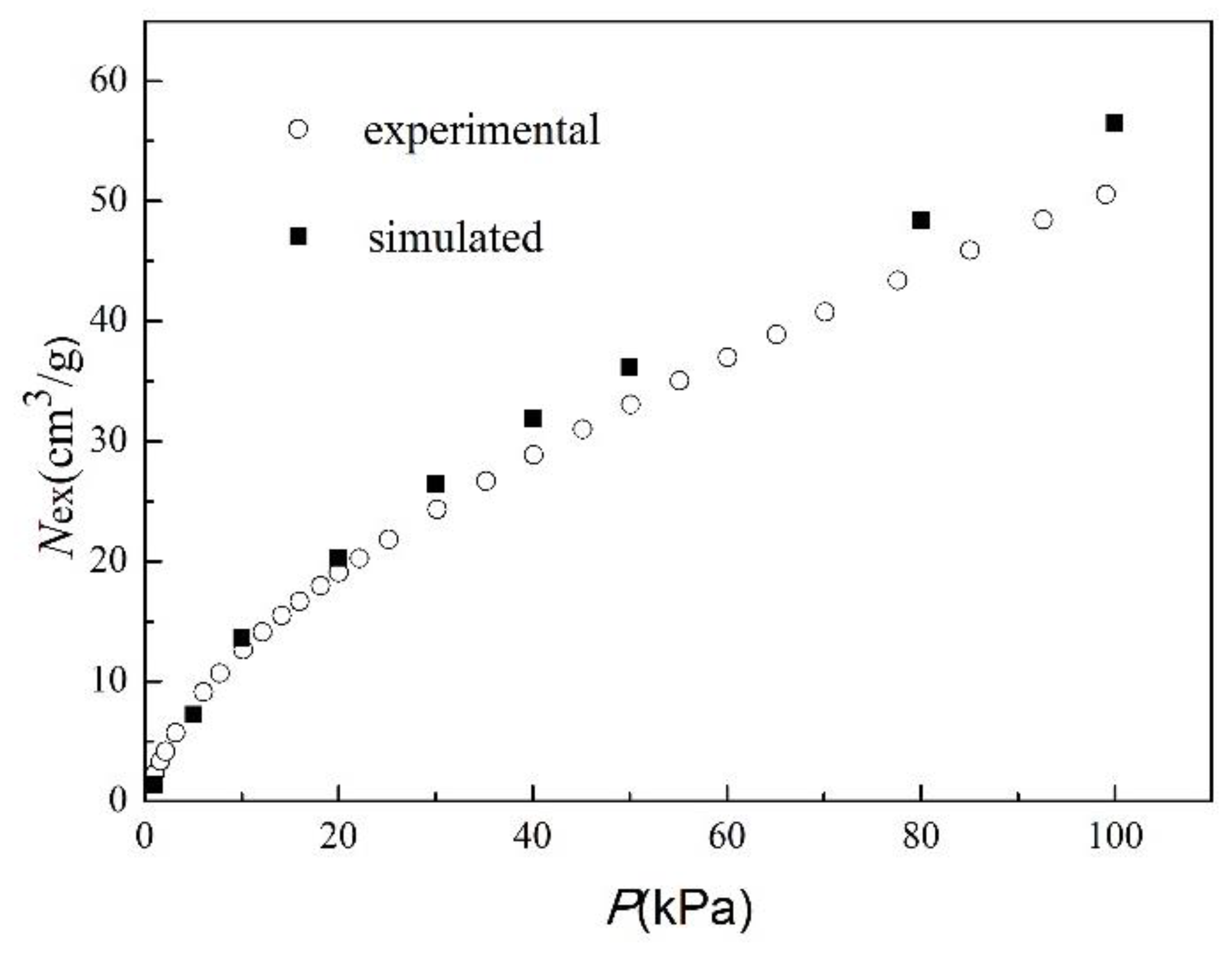
To verify the reliability of simulation results, the simulated adsorption isotherms of CO₂ on MIL-101 (Cr) at 298 K were compared to experimental data [33,34]. As shown in Figure 3, the simulated adsorption isotherms were slightly higher than the experimental values, and the deviation from the experimental value increased with the increase of pressure. These phenomena provide reasonable explanations: (1) the model of MIL-101 (Cr) that was used in the calculations contained no crystal defects and no impurities. However, actual MIL-101 (Cr) may have defects, and its pores may contain residual terephthalic acid, which can result in a relatively low CO₂ adsorption capacity; (2) when the pressure was low, the CO₂ adsorption capacity on MIL-101 (Cr) was also low, CO₂ molecules only occupied a small amount of space, and the residual impurities in the pores had little effect on the adsorption capacity. With the increase of pressure, the adsorption capacity also increased, and CO₂ molecules occupied more and more space in the pores. The existence of impurities hindered the adsorption of CO₂, resulting in the increase of deviation between the experimental and simulated values. In addition,

Table 5. The adsorption capacities and adsorption energies of CO₂ on MIL-101 (Cr) under different pressures at 298 K.

Pressure (kPa)	Average Adsorption Capacity (cm3·g−1 STP)	Standard Deviations (cm3·g−1 STP)	Coulomb Energy (kJ·moL−1)	Van Der Waals Energy (kJ·moL−1)	Total Energy (kJ·moL−1)
10	14.22	0.1594	−2.59	−21.03	−23.62
20	21.46	0.1476	−2.65	−20.53	−23.17
50	36.71	0.1538	−2.79	−19.42	−22.21
100	57.38	0.1627	−3.02	−18.73	−21.76
200	88.67	0.1653	−3.13	−16.97	−20.11
300	119.64	0.1748	−3.11	−15.55	−18.66

shows the standard deviations of adsorption capacity. The value of the standard deviations of adsorption capacity are all less than 0.2, which indicated that the results could be repeated and the MC method could be applied to this system. Therefore, this simulation method, which is based on an MC simulation in a grand canonical ensemble, was utilized for further study, and the simulation results were considered to be accurate and reliable.

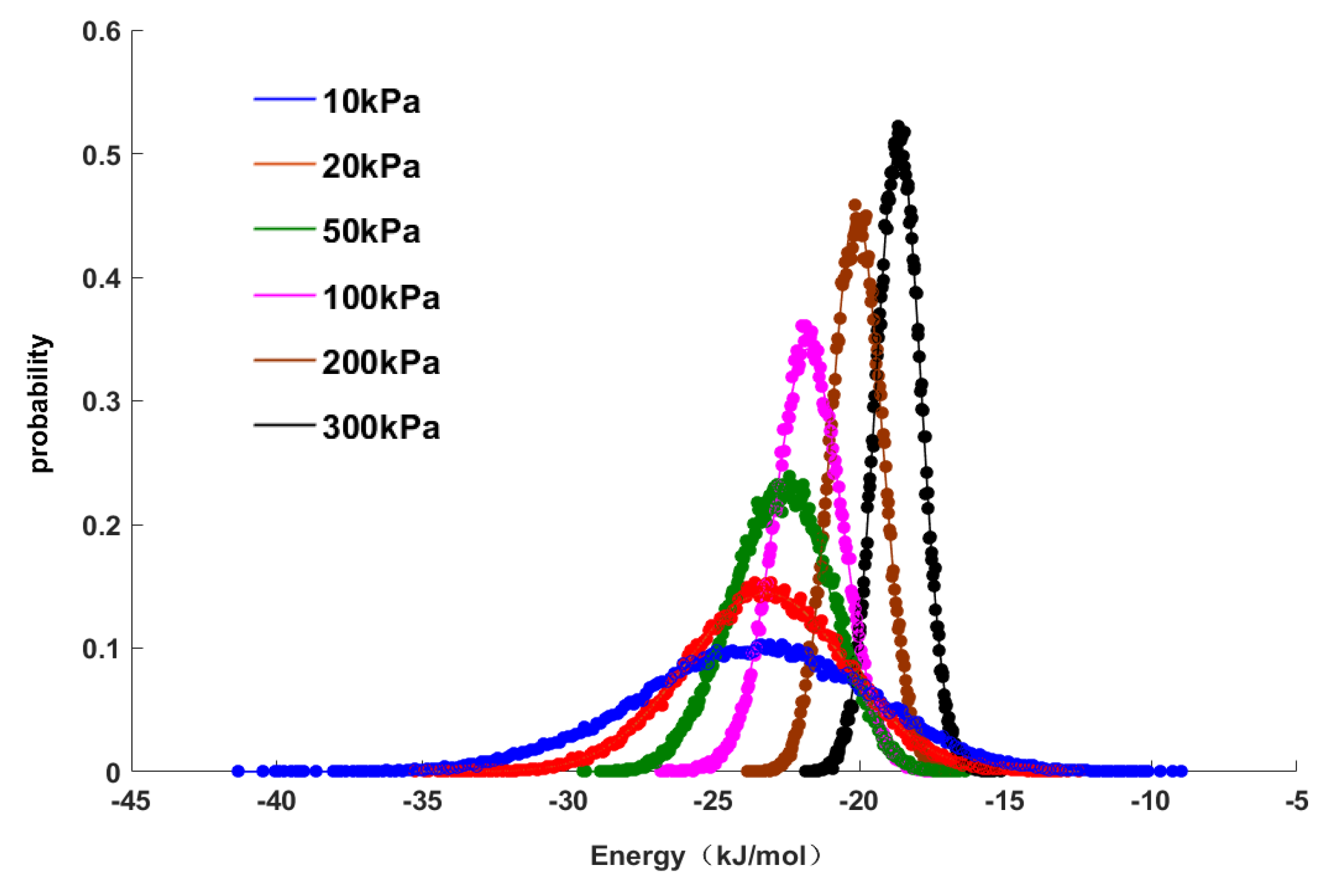
When calculating the adsorption isotherm, the adsorption energy reflecting the strength of the interaction between an adsorbent and an adsorbate can also be obtained. In this process, the adsorption energy was not constant. As summarized in Table 5, the absolute value of the adsorption energy decreased, as the pressure increased, indicating that the interaction between the adsorbent and the adsorbate decreased as the pressure and adsorption capacity increased. Figure 4 shows the characteristics and distributions of the adsorption energy. The data points in Figure 4 represent the distribution points of the adsorption energy characteristics determined by GCMC molecular simulations, and the curve represents the curve fitted by a normal distribution model in the mathematical software MATLAB to correlate all data points. It can be seen in Figure 4 that the normal distribution model had a good regression effect for the data points. Under different pressures, the values of the distributions of adsorption energy were different, but they all obeyed a normal distribution. The purpose of this study is to explore the relationship between adsorption energy and pressure, so the average value of the adsorption energy was used in subsequent work and is shown as the peak value of the normal distribution (Figure 4). As the pressure increased, the peak value of the normal distribution shifted to the right, and the distribution area of adsorption energy narrowed, that is, the absolute average value of adsorption energy decreased. 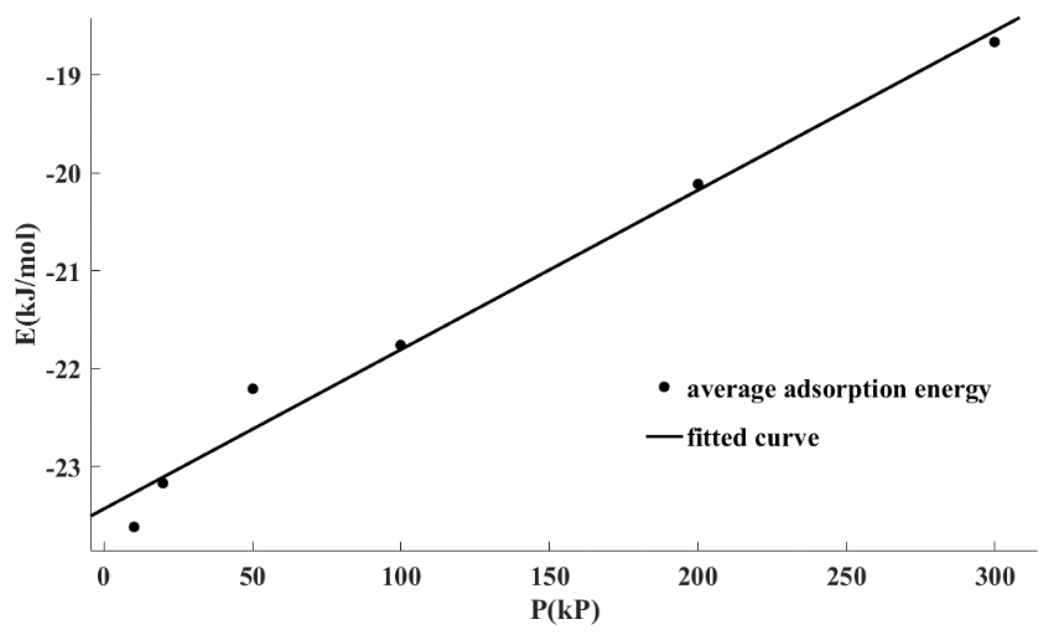This result indicated that the adsorption was gradually weakened, which was also consistent with the change in adsorption energy shown in Table 5. From the above results, it can be seen that the average adsorption energy was correlated with the adsorption pressure, that is, there was a linear relationship between them that can be expressed as follows:

$$E=aP+c,$$

(3)

where E is the average adsorption energy, P is the adsorption pressure, and a and c are the coefficients of the linear relationship between the adsorption energy and the adsorption pressure.

Figure 5 shows the fitting correlation curve of the average adsorption energy data points under different pressures using Equation (3). It can be seen that Equation (3) can well describe the relationship between the adsorption energy and pressure. It also can be seen from

Table 6. Parameters of and errors in the linear regression for average adsorption energy.

a (J·moL−1·Pa−1)	C (kJ·moL−1)	R	R2	SSE
0.01687	−23.61	0.9936	0.9873	0.1217

that the determination coefficient (R²) for linear regression was greater than 0.98 and the residual sum of squared estimate of errors (SSE) was only 0.12. In conclusion, there was a linear relationship between the adsorption energy and the adsorption pressure, which can be written as Equation (3).

4.2. Modification of the DSL Model

The form of the DSL adsorption equilibrium model [3,35,36,37] was shown as follows:

$$q=\frac{q_{m1}{b}_{1}P}{1+b_{1}P}+\frac{q_{m2}{b}_{2}P}{1+b_{2}P},$$

(4)

where P is the adsorption equilibrium pressure, q is the adsorption capacity at an equilibrium pressure, q_m1 and q_m2 represent the saturated adsorption capacities at adsorption sites 1 and 2, respectively, and b₁ and b₂ represent the Langmuir adsorption equilibrium constants of adsorption site 1 and 2, respectively, which can be written as follows:

$$b_i=k_i\exp \left(\frac{E_i}{RT}\right)(i=1,2),$$

(5)

where k_i is a pre-exponential factor, R is the gas constant, and T is the adsorption temperature.

Equation (6) can be obtained by combining Equations (3) and (5):

$$b_i=k_i\exp \left(\frac{a_{i}P+c_i}{RT}\right)(i=1,2).$$

(6)

By substituting Equation (6) into Equation (4), a new modified DSL model (M-DSL) without the adsorption energy E as a parameter can be obtained. The form of the M-DSL model was described as follows:

$$q=\frac{q_{m1}{k}_1\exp (\frac{a_{1}P+c_1}{RT})P}{1+k_1\exp (\frac{a_{1}P+c_1}{RT})P}+\frac{q_{m2}{k}_2\exp (\frac{a_{2}P+c_2}{RT})P}{1+k_2\exp (\frac{a_{2}P+c_2}{RT})P}.$$

(7)

Because there are many parameters in Equation (7), it can be simplified by combining relevant parameters. The simplification was expressed in Equation (8), which was the simplified form of the M-DSL model:

$$q=\frac{q_{m1}{k}_{m1}\exp (a_{m1}P)P}{1+k_{m1}\exp (a_{m1}P)P}+\frac{q_{m2}{k}_{m2}\exp (a_{m2}P)P}{1+k_{m2}\exp (a_{m2}P)P},$$

(8)

where k_m1 and k_m2 are two new parameters that are obtained by multiplying k_i by e^ci/RT, and a_m1 and a_m2 are two new coefficients of the linear relationship between the adsorption energy and pressure.

4.3. Regression of Adsorption Equilibrium Data with the DSL Model and the M-DSL Model

The DSL model and the M-DSL model were used to regress the adsorption equilibrium data by the nonlinear regression method, and the corresponding model parameters were obtained. The nonlinear regression was realized by the lsqnonlin function in MATLAB, and we used the Levenberg–Marquardt algorithm. The results were calculated with Equation (9), which was written as:

$$\min {{\displaystyle \sum _{i=1}^N\left(q_{i,exp}-q_{i,pre}\right)}}^2,$$

(9)

where i is the number of experimental data points, N is the total number of experimental data points, q_i,exp is the experimental value, and q_i,pre is the regression value. The lsqnonlin function in MATLAB is based on the nonlinear least squares method. In the process of regression using this method, the selection of an initial value is very important, different initial values may obtain different results. The specific operation process is as follows: (1) an appropriate initial value is selected according to experience of regression calculation; (2) the results of the first regression are taken as the initial values of regression; and (3) regression is carried out, until the obtained model parameter value no longer changes. After the operation process is completed, the R² of the model reaches the maximum, and the SSE has the minimum value, and the results are the final model parameter values. Therefore, using this method to regress the same system could get the same results, which showed that the results had good repeatability, and the model parameters obtained by this method were considered to be accurate and reasonable.

The accuracy of the regression was evaluated by the square sum of the error between the original experimental data and the fitting data, that is, the SSE, which was shown in Equation (10):

$$SSE={{\displaystyle \sum _{i=1}^N\left(y_{i,exp}-y_{i,pre}\right)}}^2,$$

(10)

where i is the number of experimental data points, N is the total number of experimental data points, y_i,exp is the experimental value, and y_{i, pre} is the regression value. The closer the SSE is to 0, the closer the predicted values of the model are to the experimental values, and the better the model describes the experimental data.

The square of the correlation coefficient (R²) can also be used as an evaluation index of data fitting. It is defined as the ratio of the sum of squares of the fitting deviation to the sum of squares of the actual deviation and can be calculated with Equation (11):

$$R^2=\frac{{\displaystyle \sum _{i=1}^N{\left(y_{i,pre}-\overline{y}\right)}^2}}{{\displaystyle \sum _{i=1}^N{\left(y_{i,exp}-\overline{y}\right)}^2}},$$

(11)

where i is the number of experimental data points, N is the total number of experimental data points, y_i,exp is the experimental value, y_i,pre is the regression value, and ȳ is the average number of experimental values used to determine the adsorption capacity. R² ranges from 0 to 1. The smaller the value is, the worse the fit between the model and the data is; the closer the value is to 1, the better the fit of the model is. In this study, SSE and R² were combined in order to analyze the regression results.

We used the adsorption equilibrium data on C₂H₄-HHPAC, CO₂-MIL-101 (Cr), CH₄-BPL active carbon, and a CO₂-H-Mordenite molecular sieve [31,32], as determined by experiments, in the DSL model and the M-DSL model for the nonlinear regression. The reason why we selected these data is that they have a wide range of adsorption temperatures and pressures and are commonly used to test adsorption equilibrium models. In addition, the adsorbents used in these systems are commonly used in industry, among which BPL is cylindrical, H-Mordenite is spherical and HHPAC is powder. Therefore, the shapes of adsorbents selected in this study almost contained the shapes of adsorbents commonly used in industry. Similarly, the adsorbates in these systems contained common organic gases such as CH₄ and C₂H₄ and common inorganic gas CO₂. Therefore, it could be said that the adsorption systems studied in this paper were sufficiently comprehensive, and the conclusions could be applied to most systems in industry.

Supplementary Figure S1 compares the correlation curves of the DSL model and the M-DSL model for different systems.

Table 7. The dual-site Langmuir (DSL) model parameters and errors for different systems at different temperatures.

Adsorbent	Adsorbate	T (K)	qm1 (mmoL·g−1)	qm2 (mmoL·g−1)	b1 (kPa−1)	b2 (kPa−1)	R2	SSE
HHPAC	C2H4	223.15	3.227	3.594	$4.827\times {10}^{-3}$	0.5834	0.9838	0.8008
		233.15	3.296	3.192	$3.243\times {10}^{-3}$	0.3121	0.9839	0.8031
		253.15	2.835	2.712	$3.057\times {10}^{-3}$	0.1623	0.9969	0.2260
		273.15	2.862	1.975	$3.904\times {10}^{-3}$	0.1292	0.9984	0.1029
		293.15	1.483	2.785	$9.336\times {10}^{-2}$	0.1366	0.9989	$3.262\times {10}^{-2}$
		313.15	0.9042	3.284	0.1411	0.1921	0.9848	0.6034
MIL-101	CO2	298.15	3.897	1.616	$1.012\times {10}^{-2}$	0.2223	0.9817	0.3605
		212.15	3.394	4.571	$3.426\times {10}^{-2}$	$1.906\times {10}^{-3}$	0.9994	$4.943\times {10}^{-2}$
BPL	CH4	260.15	2.011	4.693	$9.204\times {10}^{-3}$	$9.796\times {10}^{-4}$	0.9998	$1.294\times {10}^{-2}$
		303.15	4.871	0.6452	$7.897\times {10}^{-3}$	$6.927\times {10}^{-4}$	0.9998	$5.823\times {10}^{-3}$
		283.15	2.226	0.7744	$3.896\times {10}^{-3}$	0.2279	0.9995	$3.815\times {10}^{-3}$
H-Mordenite	CO2	303.15	0.7093	2.275	$9.077\times {10}^{-2}$	0.1922	0.9991	$1.772\times {10}^{-3}$
		323.15	2.554	0.6086	$8.113\times {10}^{-2}$	0.4426	0.9991	$1.534\times {10}^{-2}$

and

Table 8. The modified DSL (M-DSL) model parameters and errors for different systems at different temperatures.

Adsorbent	Adsorbate	T (K)	qm1 (mmoL·g−1)	qm2 (mmoL·g−1)	km1 (kPa−1)	km2 (kPa−1)	am1 (kPa−1)	am2 (kPa−1)	R2	SSE
HHPAC	C2H4	223.15	3.487	3.553	$3.441\times {10}^{-3}$	0.3387	$1.131\times {10}^{-2}$	$1.006\times {10}^{-3}$	0.9958	0.3265
		233.15	3.084	3.555	$2.312\times {10}^{-3}$	0.1709	$3.202\times {10}^{-3}$	$1.293\times {10}^{-2}$	0.9965	0.2752
		253.15	3.002	2.674	$2.249\times {10}^{-3}$	0.1092	$1.413\times {10}^{-3}$	$1.907\times {10}^{-4}$	0.9981	0.1362
		273.15	2.639	2.188	$3.516\times {10}^{-3}$	$8.951\times {10}^{-2}$	$6.299\times {10}^{-4}$	$3.912\times {10}^{-4}$	0.9989	$6.423\times {10}^{-2}$
		293.15	2.686	1.542	$3.706\times {10}^{-3}$	$7.905\times {10}^{-2}$	$1.046\times {10}^{-4}$	$3.232\times {10}^{-5}$	0.9994	$2.931\times {10}^{-2}$
		313.15	2.462	1.276	$2.972\times {10}^{-3}$	$5.514\times {10}^{-2}$	$1.996\times {10}^{-5}$	$6.359\times {10}^{-5}$	0.9992	$3.271\times {10}^{-2}$
MIL-101 (Cr)	CO2	298.15	4.431	1.863	$8.564\times {10}^{-3}$	0.3527	$1.859\times {10}^{-2}$	$1.768\times {10}^{-2}$	0.9999	$9.938\times {10}^{-4}$
		212.15	4.587	3.539	$1.765\times {10}^{-3}$	$3.254\times {10}^{-2}$	$1.499\times {10}^{-6}$	$4.802\times {10}^{-4}$	0.9994	$4.923\times {10}^{-2}$
BPL	CH4	260.15	4.694	2.528	$7.703\times {10}^{-4}$	$7.342\times {10}^{-3}$	$3.104\times {10}^{-6}$	$4.228\times {10}^{-4}$	0.9998	$9.712\times {10}^{-3}$
		303.15	6.721	2.434	$2.554\times {10}^{-4}$	$2.377\times {10}^{-3}$	$2.764\times {10}^{-5}$	$6.213\times {10}^{-4}$	0.9999	$3.534\times {10}^{-3}$
		283.15	2.168	0.7476	$4.312\times {10}^{-4}$	0.2434	$5.731\times {10}^{-3}$	$7.365\times {10}^{-2}$	0.9995	$3.724\times {10}^{-3}$
H-Mordenite	CO2	303.15	2.275	0.7091	$1.921\times {10}^{-2}$	0.9082	$1.285\times {10}^{-3}$	$3.498\times {10}^{-3}$	0.9991	$1.572\times {10}^{-2}$
		323.15	2.515	0.6459	$7.876\times {10}^{-3}$	0.3649	$2.544\times {10}^{-3}$	$5.753\times {10}^{-3}$	0.9992	$1.385\times {10}^{-2}$

show the corresponding parameter values that were obtained by the regression of the adsorption equilibrium data on each system by using the DSL and M-DSL models, respectively. As shown in Figure S1, for the C₂H₄-HHPAC system, the DSL model was able to relate the entire adsorption isotherm, and the regression effects were quite different under different temperatures and pressures. From Table 7 and Table 8, when the temperature was 253.15, 273.15, and 293.15 K, the DSL model was able to correlate the adsorption equilibrium data, which verified the applicability of the DSL model in the normal temperature range. However, the M-DSL model can better describe the adsorption isotherms of the system at these temperatures. The value of R² was greater than 0.998, and the SSE value was less than 0.1. By calculating the change in the SSE, we can see that the regression accuracy of the data with the M-DSL model was approximately 30% higher than that with the DSL model. These results indicated that the M-DSL model inherited the advantages of the DSL model in the normal temperature range and had better applicability.

When the temperatures were 223.15 and 233.15 K, the adsorption pressure gradually increased close to the saturated vapor pressure of C₂H₄, and, during this time, the adsorption capacity increased rapidly. At the temperature of 313.15 K, the adsorption capacity decreased significantly. These results showed that the DSL model was unable to well correlate the adsorption equilibrium data on C₂H₄-HHPAC in the low-temperature range and the high-temperature range. Under these conditions, the R² of the DSL model was only 0.98, and the SSE was greater than 0.8. However, the M-DSL model can accurately describe adsorption isotherms in the low-temperature range. The regression accuracy of the M-DSL model to the adsorption equilibrium data was improved by more than 50%, the R² was greater than 0.995, and the SSE was less than 0.3. In addition, the M-DSL model had obvious advantages in the high-temperature range. When the temperature was 313.15 K, the correlation curve of the M-DSL model was smoother than that of the DSL model. The R² of the M-DSL model increased to 0.999, the SSE decreased to 0.03, and the regression accuracy increased by 94%. We drew similar conclusions for the CH₄-BPL activated carbon and CO₂-H-Mordenite systems. The regression accuracies of the M-DSL model and the DSL model were 22% and 8%, respectively. In conclusion, in ranges, in which large changes in adsorption capacity occur, such as high-temperature or low-temperature ranges, the adsorption energy cannot be simply assumed to be constant. The M-DSL model, which takes into account the linear relationship between adsorption energy and adsorption pressure, has a wider application range than the DSL model. It is also able to correlate adsorption equilibrium data well in the low-temperature range, the high-temperature range, and a relatively high-pressure range, where the DSL model is inapplicable.

Regarding the MIL-101 (Cr)-CO₂ system, because the pore structure of the adsorbent was more complex than that of carbon materials and molecular sieves, the regression effect of the DSL model was poor. The value of R² was only 0.98, which cannot produce the expected effect. The regression effect of CO2-MIL-101 (Cr) was greatly improved when using the M-DSL model. The R² value was 0.9999, which is close to its upper limit (1), and the SSE was also very small (almost 0). The accuracy of the regression was 98% higher than that of the original DSL model. This result showed that the M-DSL model better correlated the adsorption equilibrium data on systems with a complex structure. Considering the linear relationship between the adsorption energy and pressure in an adsorption system with a complex pore structure can greatly improve the accuracy of the DSL model and improve the universality of the DSL model.

4.4. Modification of the TDSL Model That Reflects Temperature Changes

In the model parameter regression, we found that the parameters that were obtained by the DSL model and the M-DSL model were quite different at different temperatures and that the adsorption energy, which was found to have a linear relationship with the pressure obtained by a GCMC simulation, can modify the DSL model at different temperatures and had a good effect. In order to further verify this conclusion, we chose the DSL model that reflects temperature changes (TDSL), which is used in the adsorption module of Aspenplus and has been used in previous research [16,17,18], and attempted to improve its accuracy and universality. The TDSL model is a two-parameter adsorption equilibrium model that is based on the DSL model and takes temperature and pressure as variables together. It is also based on the three assumptions of the Langmuir model. With this model, the adsorption equilibrium data obtained at different temperatures in the same system can be correlated at the same time. The form of the TDSL model is shown in Equation (12):

$$q=\frac{\left(k_1+k_{2}T\right)\exp \left(\frac{k_3}{RT}\right)P}{1+k_4\exp \left(\frac{k_3}{RT}\right)P}+\frac{\left(k_5+k_{6}T\right)\exp \left(\frac{k_7}{RT}\right)P}{1+k_8\exp \left(\frac{k_7}{RT}\right)P},$$

(12)

where P is the adsorption equilibrium pressure, q is the adsorption capacity at the equilibrium pressure, R is the gas constant, T is the adsorption temperature, k₁, k₂, k₅, and k₆ are the coefficients of the linear relationship between the saturated adsorption capacity and temperature in the original DSL model, k ₃ and k₇ are the adsorption energies corresponding to different adsorption sites, and k₄ and k₈ are pre-exponential factors.

Based on the conclusion that adsorption energy has a linear relationship with pressure, the TDSL model can be modified to obtain the M-TDSL model by substituting Equation (5) into Equation (12). The form of the modified TDSL (M-TDSL) model is shown in Equation (13):

$$q=\frac{\left(k_1+k_{2}T\right)\exp \left(\frac{c_1+a_{1}P}{RT}\right)P}{1+k_4\exp \left(\frac{c_1+a_{1}P}{RT}\right)P}+\frac{\left(k_5+k_{6}T\right)\exp \left(\frac{c_2+a_{2}P}{RT}\right)P}{1+k_8\exp \left(\frac{c_2+a_{2}P}{RT}\right)P},$$

(13)

where a₁, c₁, a₂, and c₂ are coefficients of the linear relationship between the adsorption energy and the adsorption pressure. The TDSL model and the obtained M-TDSL model were used to correlate the adsorption equilibrium data of the above systems at different temperatures at the same time. The results are shown in

Table 9. The TDSL model parameters and errors for different systems.

	C2H4-HHPAC	CH4-BPL	CO2-H-Mordenite
k1 (mmoL·g−1)	8.159	2.105	1.549
k2 (mmoL·g−1·T−1)	$-2.516\times {10}^{-2}$	$-2.452\times {10}^{-3}$	$-3.351\times {10}^{-3}$
k3 (kJ·moL−1)	−19.98	−18.56	−15.84
k4 (kPa−1)	0.8338	$1.909\times {10}^{-2}$	0.2044
k5 (mmoL·g−1)	2.406	1.876	2.392
k6 (mmoL·g−1·T−1)	$-1.609\times {10}^{-4}$	$-4.402\times {10}^{-4}$	$-1.923\times {10}^{-4}$
k7 (kJ·moL−1)	−28.99	−23.85	−12.21
k8 (kPa−1)	$6.134\times {10}^{-3}$	$1.292\times {10}^{-3}$	0.1431
R2	0.9907	0.9754	0.9858
SSE	5.544	4.765	0.6422

and

Table 10. The modified TDSL (M-TDSL) model parameters and errors for different systems.

	C2H4-HHPAC	CH4-BPL	CO2-H-Mordenite
k1 (mmoL·g−1)	3.876	2.754	4.103
k2 (mmoL·g−1·T−1)	$-1.188\times {10}^{-2}$	$-9.388\times {10}^{-3}$	$-1.262\times {10}^{-2}$
k4 (kPa−1)	0.3981	0.2425	0.6967
c1 (kJ·moL−1)	−19.16	−13.35	−31.77
a1 (J·moL−1·Pa−1)	$3.497\times {10}^{-3}$	$1.892\times {10}^{-3}$	$1.086\times {10}^{-3}$
k5 (mmoL·g−1)	2.418	3.178	4.908
k6 (mmoL·g−1·T−1)	$-1.791\times {10}^{-3}$	$-6.047\times {10}^{-3}$	$-1.036\times {10}^{-3}$
k8 (kPa−1)	$6.142\times {10}^{-3}$	$1.366\times {10}^{-2}$	$6.574\times {10}^{-2}$
c2 (kJ·moL−1)	−21.39	−32.95	−25.85
a2 (J·moL−1·Pa−1)	$2.678\times {10}^{-3}$	$6.162\times {10}^{-3}$	$3.586\times {10}^{-3}$
R2	0.9912	0.9902	0.9936
SSE	4.736	3.652	0.3284

.

Supplementary Figure S2 shows the correlation curves of the TDSL model and the M-TDSL model for different systems. Table 9 and Table 10 show the corresponding parameter values that were obtained by the regression of the adsorption equilibrium data on each system by using the TDSL and M-TDSL models, respectively. Overall, the TDSL model was able to correlate the adsorption equilibrium data on CO₂-HHPAC well. Its R² was greater than 0.99, and its SSE was in a reasonable range. From the physical meaning of the parameters, it can be seen that the values of k₃ and k₇ were the adsorption energies at the two adsorption sites, respectively, and the results also showed that the adsorption energies were −19.98 and −28.99 kJ·mol⁻¹, respectively, which are in the general range of physical adsorption energies. This indicated that the regression results were reliable and accurate and that the physical meanings of the corresponding parameters were clear and definite. The regression effect of the M-TDSL model on the adsorption equilibrium data was slightly improved as compared to that of the original model, and the accuracy of the regression was increased by 14%. For the CH₄-BPL and CO₂-H-Mordenite systems, the TDSL model had a poor correlation, which cannot produce the expected effect. In fact, the M-TDSL model was better than the TDSL model with respect to the fitting correlation effects of these systems. Its R² was greater than 0.99, its SSE was significantly smaller than that of the TDSL model, and the regression accuracies of the M-TDSL and TDSL were also improved by 23% and 31%, respectively, compared with that of the original TDSL model. In the M-TDSL model, the two adsorption energies were numerically equal to the values of (c₁ + a₁P) and (c₂ + a₂P), both of which were in the general range of physical adsorption energies. In conclusion, the average regression accuracy when using the M-TDSL model was 23% higher than that when using the original TDSL model. Therefore, the obtained M-TDSL model had higher precision and a wider application range than the TDSL model, and the model parameters also had clear physical significance.

In addition, the results also showed that our conclusion—adsorption energy has a linear relationship with pressure—has certain universality across different adsorption equilibrium models. This relationship provides a basis for modifying other forms of adsorption equilibrium models and can be further tested when modifying other adsorption equilibrium models.

5. Conclusions

In this study, a GCMC molecular simulation was used to calculate the CO₂ adsorption equilibrium on MIL-101 (Cr) at 298 K, and the characteristics and distribution of adsorption energy with pressure were obtained. The calculated results showed that the adsorption energies with different adsorption pressures fitted a normal distribution and the relationship of average adsorption energies with pressures had a linear form. The linear relationship between the adsorption energies and pressure was used to modify the parameters of the DSL model, and the M-DSL model was used to correlate the adsorption equilibrium data on CO₂-MIL-101 (Cr), C₂H₄-HHPAC, CH₄-BPL, and CO₂-H-Mordenite. The results showed that the accuracy and generality of the M-DSL model were significantly improved after the modification and the average regression accuracy of the correlation of adsorption equilibrium data on each system was increased by 38%. The M-DSL model can better correlate the adsorption equilibrium data in high- or low-temperature ranges, and its correlation effect in the normal temperature range was also better than that of the DSL model. In addition, the M-DSL model showed a better correlation for systems with a more complex pore structure, such as CO₂-MIL-101 (Cr). Similar to the DSL model, the linear relationship between the adsorption energy and pressure was also used to modify the TDSL model. The obtained M-TDSL model was checked with the abovementioned adsorption equilibrium systems. The results also indicated that the M-TDSL model could be used to improve the correlation of adsorption equilibrium data obtained at different temperatures. The average accuracy of the correlation for each system was increased by 23%, and the physical meanings of the parameters in the M-DSL model were clear and definite. In the process of practical applications, the modified models would increase the number of required calculations due to their more complex form, which will become a limitation. However, their good accuracy and versatility can make up for this disadvantage. Finally, our conclusion that adsorption energy has a linear relationship with pressure provides a basis for modifying other types of adsorption equilibrium models. The linear relationship between the adsorption energy and pressure could be further tested in other adsorption equilibrium models to determine its universality.

References

1. Seidel-Morgenstern, A. Experimental determination of single solute and competitive adsorption isotherms. J. Chromatogr. A 2004, 1037, 255–272. [Google Scholar] [CrossRef] [PubMed]
2. Wong, Y.C.; Szeto, Y.S.; Cheung, W.H.; Mckay, G. Adsorption of acid dyes on chitosan—Equilibrium isotherm analyses. Process Biochem. 2004, 39, 695–704. [Google Scholar] [CrossRef]
3. Technology, NATO Advanced Study Institute. Adsorption: Science and Technology; Kluwer Academic Publishers: Amsterdam, The Netherlands, 1989; pp. 38–39. [Google Scholar]
4. Feilong, S.; Fanchao, M.; Jie, G.; Zhengfei, M. Measurement of Adsorption Equilibrium Data of Ethylene on Activated Carbon and Temperature Dependence on Parameters for Langmuir Model. J. Nanjing Technol. Univ. 2017, 39, 121–126. [Google Scholar]
5. Augelletti, R.; Conti, M.; Annesini, M.C. Pressure swing adsorption for biogas upgrading. A new process configuration for the separation of biomethane and carbon dioxide. J. Clean. Prod. 2017, 140, 1390–1398. [Google Scholar] [CrossRef]
6. Voros, V.; Drioli, E.; Fonte, C.; Szekely, G. Process Intensification via Continuous and Simultaneous Isolation of Antioxidants: An Upcycling Approach for Olive Leaf Waste. ACS Sustain. Chem. Eng. 2019, 7, 18444–18452. [Google Scholar] [CrossRef]
7. Didaskalou, C.; Buyuktiryaki, S.; Kecili, R.; Fonte, C.P.; Szekely, G. Valorisation of agricultural waste with an adsorption/nanofiltration hybrid process: From materials to sustainable process design. Green Chem. 2017, 19, 3116–3125. [Google Scholar] [CrossRef] [Green Version]
8. Tsay, C.; Pattison, R.C.; Beldea, M. A Pseudo-Transient Optimization Framework for Periodic Processes: Pressure Swing Adsorption and Simulated Moving Bed Chromatography. AIChE J. 2017, 64. [Google Scholar] [CrossRef]
9. Chunxia, L.; Qin, D.; Jianyu, G. Analysis of parameter estimation method of adsorption isotherm equation. Ion Exch. Adsorpt. 2012, 28, 211–220. [Google Scholar]
10. Lu, K. Porous and high surface area silicon oxycarbide-based materials—A review. Mater. Sci. Eng. R Rep. 2015, 97, 23–49. [Google Scholar] [CrossRef]
11. Foo, K.Y.; Hameed, B.H. Insights into the modeling of adsorption isotherm systems. Chem. Eng. J. 2010, 156, 2–10. [Google Scholar] [CrossRef]
12. Collins, K.E.; Collins, C.H.; Maroneze, C.M.; Cappovila, V.; Custodio, R. Evaluations of the BET, I-Point, and alpha-Plot Procedures for the Routine Determination of External Specific Surface Areas of Highly Dispersed and Porous Silicas. Langmuir 2011, 27, 187–195. [Google Scholar] [CrossRef] [PubMed]
13. Builes, S.; Sandler, S.I.; Xiong, R. Isosteric Heats of Gas and Liquid Adsorption. Langmuir 2013, 29, 10416–10422. [Google Scholar] [CrossRef] [PubMed]
14. Sipponen, M.H.; Pihlajaniemi, V.; Littunen, K.; Pastinen, O.; Laakso, S. Determination of surface-accessible acidic hydroxyls and surface area of lignin by cationic dye adsorption. Bioresour. Technol. 2014, 169, 80–87. [Google Scholar] [CrossRef] [PubMed] [Green Version]
15. Arvaniti, E.C.; Juenger, M.C.G.; Bernal, S.A.; Duchesne, J.; Courard, L.; Leroy, S.; Provis, J.L.; Klemm, A.; De Belie, N. Determination of particle size, surface area, and shape of supplementary cementitious materials by different techniques. Mater. Struct. 2015, 48, 3687–3701. [Google Scholar] [CrossRef] [Green Version]
16. Ntiamoah, A.; Ling, J.; Xiao, P.; Webley, P.A.; Zhai, Y. CO2 Capture by Temperature Swing Adsorption: Use of Hot CO2-Rich Gas for Regeneration. Ind. Eng. Chem. Res. 2016, 55, 703–713. [Google Scholar] [CrossRef]
17. Anisuzzaman, S.M.; Bono, A.; Krishnaiah, D.; Tan, Y.Z. A study on dynamic simulation of phenol adsorption in activated carbon packed bed column. J. King Saud Univ. Eng. Sci. 2016, 28, 47–55. [Google Scholar] [CrossRef] [Green Version]
18. Li, D.; Zhou, Y.; Shen, Y.; Sun, W.; Fu, Q.; Yan, H.; Zhang, D. Experiment and simulation for separating CO2/N2 by dual-reflux pressure swing adsorption process. Chem. Eng. J. 2016, 297, 315–324. [Google Scholar] [CrossRef]
19. Himeno, S.; Komatsu, T.; Fujita, S. High-pressure adsorption equilibria of methane and carbon dioxide on several activated carbons. J. Chem. Eng. Data 2005, 50, 369–376. [Google Scholar] [CrossRef]
20. Agostini, G.; Piovano, A.; Bertinetti, L.; Pellegrini, R.; Leofanti, G.; Groppo, E.; Lamberti, C. Effect of Different Face Centered Cubic Nanoparticle Distributions on Particle Size and Surface Area Determination: A Theoretical Study. J. Phys. Chem. C 2014, 118, 4085–4094. [Google Scholar] [CrossRef]
21. Park, J.; Lively, R.P.; Sholl, D.S. Establishing upper bounds on CO2 swing capacity in sub-ambient pressure swing adsorption via molecular simulation of metal–organic frameworks. J. Mater. Chem. A 2017, 5, 12258–12265. [Google Scholar] [CrossRef]
22. Ma, S.; Zhou, H. Gas storage in porous metal-organic frameworks for clean energy applications. Chem. Commun. 2010, 46, 44–53. [Google Scholar] [CrossRef] [PubMed]
23. Zhijing, W.; Junchao, W.; Xingle, Z.; Zhengfei, M. Molecular simulation of CO2 adsorption in amino modified MIL-101 (Cr). Chin. J. Inorg. Chem. 2018, 34, 1966–1974. [Google Scholar]
24. Wilmer, C.E.; Leaf, M.; Lee, C.Y.; Farha, O.K.; Hauser, B.G.; Hupp, J.T.; Snurr, R.Q. Large-scale screening of hypothetical metal–organic frameworks. Nat. Chem. 2012, 4, 83–89. [Google Scholar] [CrossRef] [PubMed]
25. Babarao, R.; Jiang, J. Molecular screening of metal-organic frameworks for CO2 storage. Langmuir 2008, 24, 6270–6278. [Google Scholar] [CrossRef]
26. Talu, O.; Myers, A.L. Molecular simulation of adsorption: Gibbs dividing surface and comparison with experiment. AIChE J. 2001, 47, 1160–1168. [Google Scholar] [CrossRef] [Green Version]
27. Karra, J.R.; Walton, K.S. Effect of open metal sites on adsorption of polar and nonpolar molecules in metal-organic framework Cu-BTC. Langmuir 2008, 24, 8620–8626. [Google Scholar] [CrossRef]
28. Kawakami, T.; Takamizawa, S.; Kitagawa, Y.; Maruta, T.; Mori, W.; Yamaguchi, K. Theoretical studies of spin arrangement of adsorbed organic radicals in metal-organic nanoporous cavity. Polyhedron 2001, 20, 1197–1206. [Google Scholar] [CrossRef]
29. Pianwanit, A.; Kritayakornupong, C.; Vongachariya, A.; Selphusit, N.; Ploymeerusmee, T.; Remsungnen, T.; Nuntasri, D.; Fritzsche, S.; Hannongbua, S. The optimal binding sites of CH4 and CO2 molecules on the metal-organic framework MOF-5: ONIOM calculations. Chem. Phys. 2008, 349, 77–82. [Google Scholar] [CrossRef]
30. Dubbeldam, D.; Calero, S.; Ellis, D.E.; Snurr, R.Q. RASPA: Molecular simulation software for adsorption and diffusion in flexible nanoporous materials. Mol. Simul. 2016, 42, 81–101. [Google Scholar] [CrossRef] [Green Version]
31. Dueren, T.; Bae, Y.; Snurr, R.Q. Using molecular simulation to characterise metal-organic frameworks for adsorption applications. Chem. Soc. Rev. 2009, 38, 1237–1247. [Google Scholar] [CrossRef]
32. Chowdhury, P.; Mekala, S.; Dreisbach, F.; Gumma, S. Adsorption of CO, CO2 and CH4 on Cu-BTC and MIL-101 metal organic frameworks: Effect of open metal sites and adsorbate polarity. Microporous Mesoporous Mater. 2012, 152, 246–252. [Google Scholar] [CrossRef]
33. Munusamy, K.; Sethia, G.; Patil, D.V.; Rallapalli, P.B.S.; Somani, R.S.; Bajaj, H.C. Sorption of carbon dioxide, methane, nitrogen and carbon monoxide on MIL-101(Cr): Volumetric measurements and dynamic adsorption studies. Chem. Eng. J. 2012, 195, 359–368. [Google Scholar] [CrossRef]
34. Jaroniec, M. Physical Adsorption on Heterogeneous Solids; Elsevier: Amsterdam, The Netherlands, 1988; pp. 11–15. [Google Scholar]
35. Villieras, F.; Cases, J.M.; Francois, M.; Michot, L.J.; Thomas, F. Texture and surface energetic heterogeneity of solids from modeling of low-pressure gas-adsorption isotherms. Langmuir 1992, 8, 1789–1795. [Google Scholar] [CrossRef]
36. Yaping, Z.; Li, Z. High pressure adsorption isotherm model of hydrogen in large temperature range. J. Chem. Eng. Chin. Univ. 1998, 3, 2–5. [Google Scholar]
37. Valenzuela, D.P. Adsorption Equilibrium Data Handbook; Prentice Hall: Guildford, UK, 1989; pp. 35–48. [Google Scholar]
Figure 1. Structures of the MIL-101 (Cr) crystal and cluster.
Applsci 10 01311 g001
Figure 2. The structure of the MIL-101 (Cr) cluster used for calculating charges.
Applsci 10 01311 g002
Figure 3. A comparison of the simulated and experimental adsorption isotherms of CO2 on MIL-101 (Cr) at 298 K.
Applsci 10 01311 g003
Figure 4. The adsorption energy distribution curves of CO2 on MIL-101 (Cr) under different pressures.
Applsci 10 01311 g004
Figure 5. Linear regression curve for the average adsorption energies of CO2 on MIL-101 (Cr) under different pressures.
Applsci 10 01311 g005