Application of Artificial Neural Networks in Assessing Mining Subsidence Risk

Abstract

Subsidence at abandoned mines sometimes causes destruction of local areas and casualties. This paper proposes a mine subsidence risk index and establishes a subsidence risk grade based on two separate analyses of A and B to predict the occurrence of subsidence at an abandoned mine. For the analyses, 227 locations were ultimately selected at 15 abandoned coal mines and 22 abandoned mines of other types (i.e., gold, silver, and metal mines). Analysis A predicts whether subsidence is likely using an artificial neural network. Analysis B assesses a mine subsidence risk index that indicates the extent of risk of subsidence. Results of both analyses are utilized to assign a subsidence risk grade to each ground location investigated. To check the model’s reliability, a new dataset of 22 locations was selected from five other abandoned mines; the subsidence risk grade results were compared with those of the actual ground conditions. The resulting correct prediction percentage for 13 subsidence locations of the abandoned mines was 83–86%. To improve reliability of the subsidence risk, much more subsidence data with greater variations in ground conditions is required, and various types of analyses by numerical and empirical approaches, etc. need to be combined.

1. Introduction

Various types of subsidence can occur at abandoned mines, especially when proper post-mining measures, such as filling the mine cavern with infilling material, are not implemented to prevent future collapse. Subsidence sometimes leads to significant consequences, including devastating ground settlement resulting in damage to the local area and also human casualties. A significant obstacle in handling subsidence at abandoned mines is predicting when and where the ground movement will occur, which significantly hinders development in the area. Accurate predictions of dynamic surface movement and deformation are exceptionally difficult because mining activity is a space–time process and dynamic surface movement is related to a wide range of factors [1].

Accordingly, many attempts have been made to more precisely predict subsidence and validate the stability of mining and land areas by numerical analyses [1,2,3,4,5], theoretical and experimental solutions [6,7,8,9,10], and/or statistical approaches [11,12], but the results have been limited because abandoned mines are generally too large and the goafs are too complex for effective analysis using the aforementioned approaches.

Against this background, the use of neural networks in fields of engineering has become prevalent in the last few years [13,14,15,16]. An artificial neural network (ANN) is a computational mechanism capable of acquiring, representing, and computing a mapping from one multivariate space of information to another, given a set of data representing that mapping [17].

ANN provides tools for optimising operations, equipment selection, and problems involving large amounts of information that humans cannot easily assimilate in the process of decision-making. Hence, the neural network can serve as a tool for determining the relative importance of the factors influencing the stability of underground objects [18].

Since the 1990s, when a number of ANN-based systems were introduced in the mining industry [19], ANN has significantly improved the current approach towards predicting abandoned mine subsidence risk [20,21,22,23]. In particular, Oh et al. [24] evaluated the performance of predictive Bayesian, functional, and meta-ensemble machine learning models in generating land subsidence susceptibility maps. Kim et al. [25] also constructed a hazard map for possible ground subsidence around abandoned underground coal mines in Korea using an ANN together with a geographic information system (GIS). Zhao and Chen [26] used an ANN to predict ground subsidence at a metal mine because ground subsidence is influenced by many factors which are fuzzy and nonlinear, and the ANN has a great function to be able to handle such nonlinear problems, without knowing specific mine conditions.

Meanwhile, Mine Reclamation Corporation (MIRECO) who is responsible for the safety and management of abandoned mines and implements mine reclamation projects in Korea has made several attempts to reliably predict subsidence by numerical, statistical, probabilistic, and/or model approaches [27,28,29,30,31] prior to this study. However, the prediction results were not up to par with MIRECO’s standards because they were not appropriate for the assessment of many as well as extensive abandoned mines.

Finally, MIRECO decided to adopt ANN as well to predict subsidence considering the merits of ANN mentioned above. Hence, the main objective of this study is to predict the possibility of subsidence on any ground under which a goaf exists by subsidence risk grade that represents the likelihood of subsidence using ANN. This study can be used as an initial method screening the specific locations that are at highest risk of subsidence and thus require immediate detailed investigation, from an extensive mine area for subsequent detailed analyses by the other approaches.

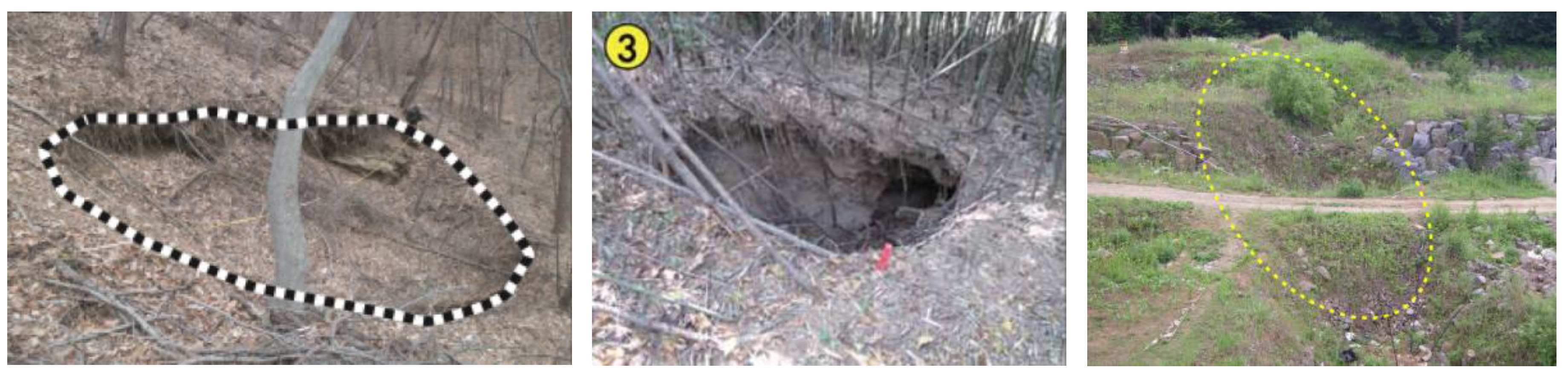
Meanwhile, from a civil engineering point of view, mining induced ground subsidence is described by parameters measuring ground deformation i.e., radius of curvature, tilt, and vertical as well as horizontal ground deformation [32,33]. The subsidence in this study signifies the big downward movement of ground’s surface enough for one to be able to easily recognize, and Figure 1 shows several examples of the subsidence.

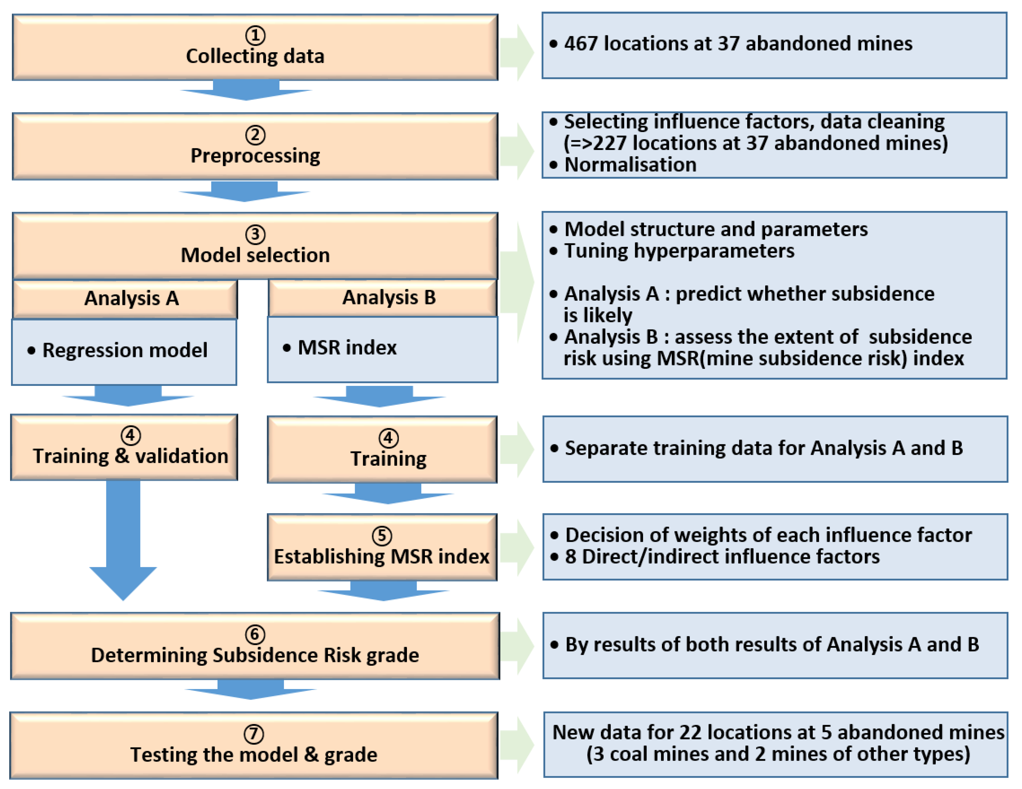
2. Methodology

The overall study process is summarized in Figure 2 and is classified into four categories; collection and preprocessing of subsidence data, construction of ANN model and training, establishment of subsidence risk grade, and test of the model with new data.

2.1. Basic Principle of ANN

The capability of an ANN model to optimize, determine, and predict a given situation depends heavily on the reliability of the database it draws from as well as the amount of data it has processed. This is because an ANN system derives its output from patterns recognized during the pre-learning stage so that a more reliable outcome can be acquired from a model that has learned from a more extensive variety of situations.

Figure 3 shows a model of the artificial neuron or processing element (PE) forming the basis of the ANN structure. This layered structure is the most common structure in ANNs and is usually called the fully connected feedforward or acyclic network. The starting point of the ANN structure is a layer of input units that allows entrance of information into the network. Normalization is the process of equalizing the signal range of different inputs. Normalization ensures that changes in the signals of different inputs have the same effect on the network’s behavior regardless of their magnitude [19].

Learning from examples is the main operation of any ANN. In this case, ‘learning’ means the ability of an ANN to improve its performance through an interactive process of adjusting its free parameters. The adjustment of an ANN’s free parameters is stimulated by a set of examples presented to the network during the application of a set of well-defined rules, called a learning algorithm, for improving its performance. There are many different learning algorithms for ANNs, each with different ways of adjusting the synaptic weights of PEs and different ways of formalizing the measurement of the ANN’s performance [19].

In general, there are three major learning algorithms: supervised learning, unsupervised learning, and reinforcement learning [34]. In supervised learning, the network is trained by providing it with input and matching output patterns. These input output pairs can be provided by an external teacher or by the system that contains the neural network (self-supervised). This study adopted supervised learning. Furthermore, there are two different approaches: error back-propagation algorithms, a gradient method, and a genetic algorithm, which is a stochastic search method [35]. The back-propagation training algorithm is the most frequently used neural network method [36,37,38]. It is trained using a set of examples of associated input and output values.

After the ANN reaches the required performance by learning examples, it can be used to predict the outcome of situations given specific input parameters. It merely behaves as a series of functions that produce an output for a particular input.

2.2. ANN Software for this Study

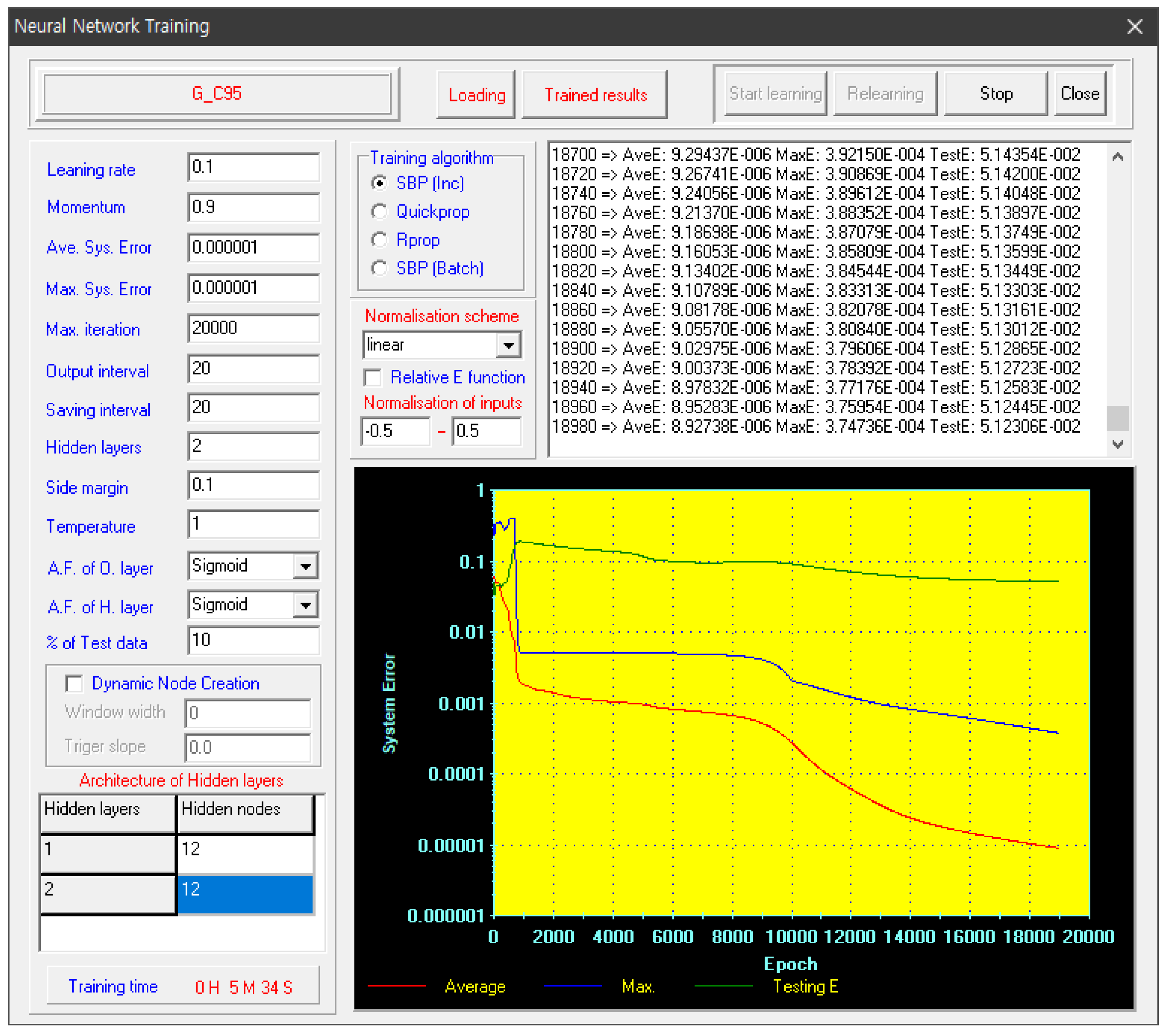
The software used for this study was the Generalized Data Analyzer and Predictor (GDAP, Ver. 2.0, 2005) developed by the University of Wales Swansea in Wales, which has been used for prediction, supervised learning, and design of structure [39]. Figure 4 shows a typical example of GDAP training, which consists of the learning rate, architecture of the hidden layer, training algorithm, normalization scheme, etc.

3. Information on/about Abandoned Mines and Datasets

The subsidence data for this study were collected from 467 locations (one location means one subsidence point), among which subsidence had occurred at 388 locations, and there were 79 locations where subsidence had not occurred (

Table 1. Number of data investigated.

		Total (37)			At Coal Mines (15)			At Other Mines (22)
		Sum	Subsidence		Sum	Subsidence		Sum	Subsidence
			Yes	No		Yes	No		Yes	No
Total collected data		467	388	79	300	257	43	167	131	36
Selected data	Sum	227	166	61	118	92	26	109	74	35
	Training	207	149	58	106	82	24	101	67	34
	Validation	20	17	3	12	10	2	8	7	1

). However, more than a few data points did not have any information on the goafs—e.g., the depth from ground to goaf, goaf height/width, and rock mass quality (RMR)—which has an essential impact on subsidence, or the information was very unclear. Such data were excluded from the analyses.

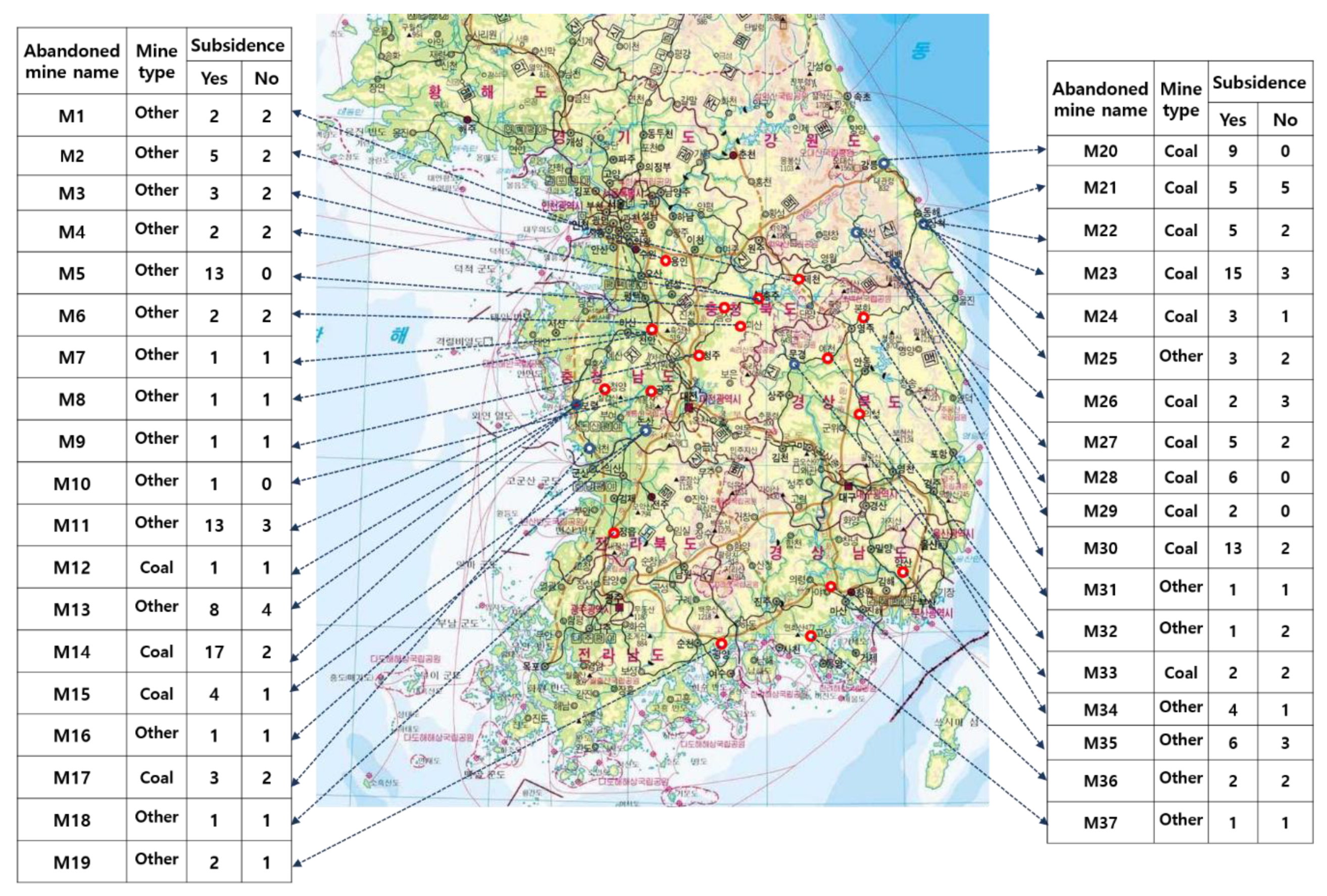
Eventually, 227 locations from 37 abandoned mines were selected for the study. Among these, 118 locations were from 15 abandoned coal mines and 109 locations were from other types of mines (i.e., gold, silver, metal). The numbers of locations that did and did not display subsidence were 166 and 61, respectively.

The locations of the selected abandoned mines are shown in Figure 5.

Furthermore, 207 of the total 227 locations were used for machine learning, and the other 20 were used for validation of the prediction model during the machine learning process. The information on the mines and subsidence locations was collected from various mine reports published by the Mine Reclamation Corporation in Korea. The reports present the results of extensive investigations on subsidence conducted at various abandoned mines across the country.

Meanwhile, many previous studies have identified important factors that contribute to ground subsidence around mines, including the depth and height of the mined cavities, excavation method, degree of inclination of the excavation, scope of mining, structural geology, and flow of groundwater [40,41]. Salmi et al. [3] found that gradual deterioration due to weathering plays a significant role in the propagation of the cavity and the formation of sinkholes above abandoned mine workings. Tzampoglou and Loupasakis [4] have analyzed the causes of 4 km long land subsidence around the mine causing damage to villages of Greece using the PLAXIS three-dimensional finite element code, and concluded that the factors which affect land subsidence (from the most dangerous to the least dangerous) are the groundwater drawdown, the geotechnical behavior of the formation, the tectonic structure, and the offset of the faults. Manekar and Chaudhari [2] mentioned that subsidence is a time-dependent process and controlled by various factors including methods of mining, depth of extraction, thickness of deposit, and topography, as well as the in-situ properties of the rock mass. Yu et al. [9] concluded that factors of the relationship between surface dynamic subsidence and overburden separated strata include the requirement of abscission layer development (stress, stiffness, mining condition, and deflection) and surface subsidence conditions (mining thickness, mining depth, mining overburden rock properties, speed). Wang et al. [10] developed a new time function model to predict the dynamic subsidence that occurs in the grout-injected overburden of a coal mine during overburden grout injection mining. This function includes the mining parameters (the width of the working face and the advancement length of the filled area), a geological parameter (the angle of full subsidence), grout injection parameters, and other relevant coefficients. Li et al. [1] mentioned that factors related to subsidence are mining and geological conditions, mining methods, working face advance speeds, and mining period, amongst others.

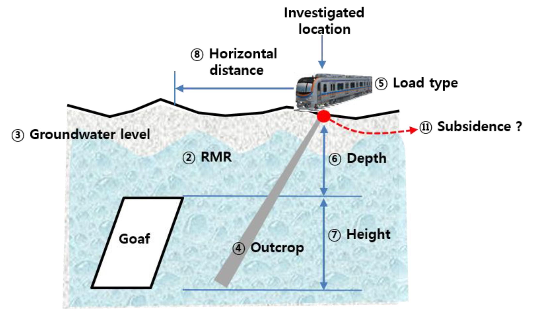
Based on the literature study regarding the factors affecting subsidence, the following 11 potential influence factors for subsidence were identified: ① elapsed time in years from the closing of the mine until an investigation was performed; ② RMR; ③ groundwater level; ④ existence of an outcrop at the investigated location; ⑤ types of loads near the investigated location (bridge, railway, house, etc.); ⑥ depth from ground to the nearest goaf; ⑦ goaf height; ⑧ horizontal distance from the investigated location to the nearest goaf; ⑨ uniaxial compressive strength (UCS) of the rock mass; ⑩ rainfall of the local area; and ⑪ occurrence or lack of occurrence of subsidence.

As the second step of data pre-processing, correlation analyses between subsidence occurrence and the potential influential factors were conducted and the multicollinearity among the factors was assessed. Multicollinearity is when two or more of the independent variables being fed into the model are highly correlated. In regression models, this may cause regression coefficients to change erratically in response to small changes in the model or the data because of confounding between the influences of highly correlated factors. Thus, if the highly correlated input variables are identified and eliminated in advance, then the network can determine the most appropriate weights more efficiently [42].

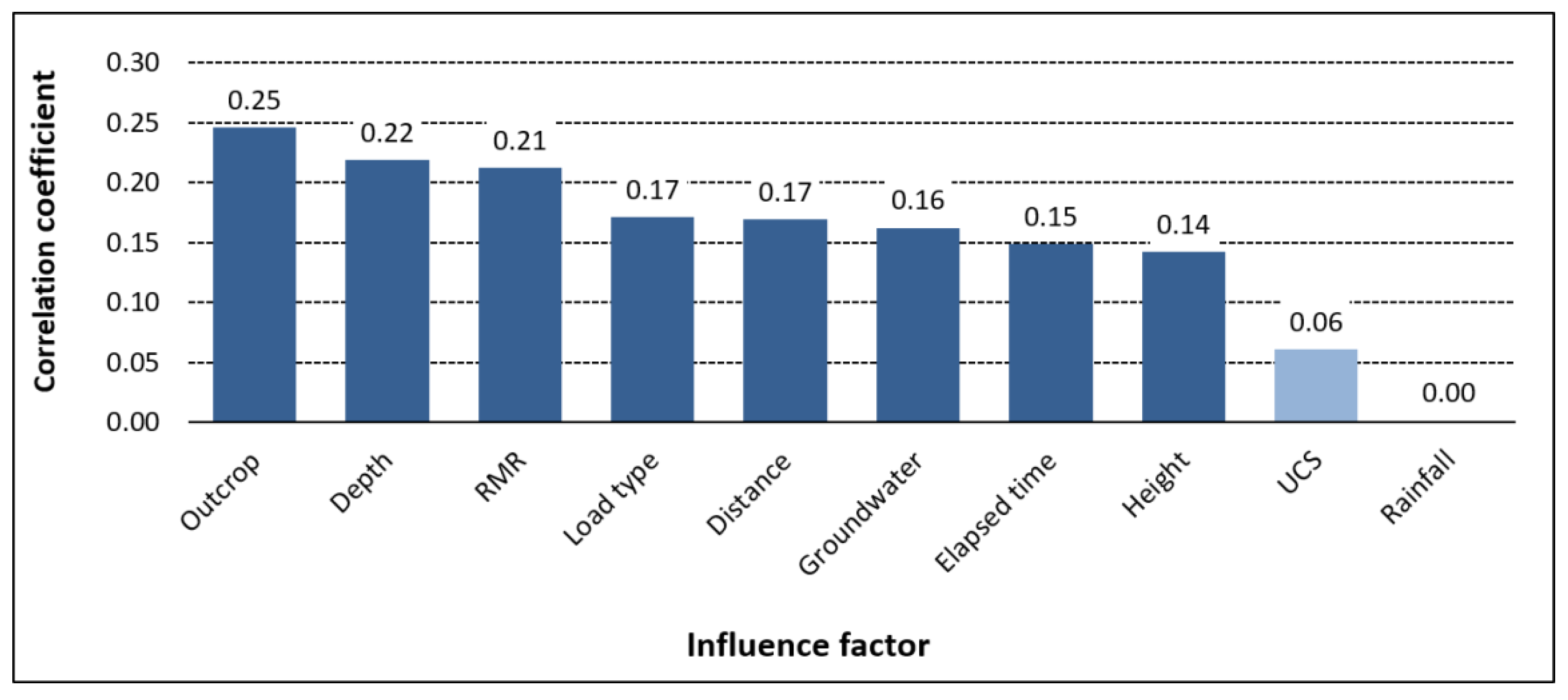
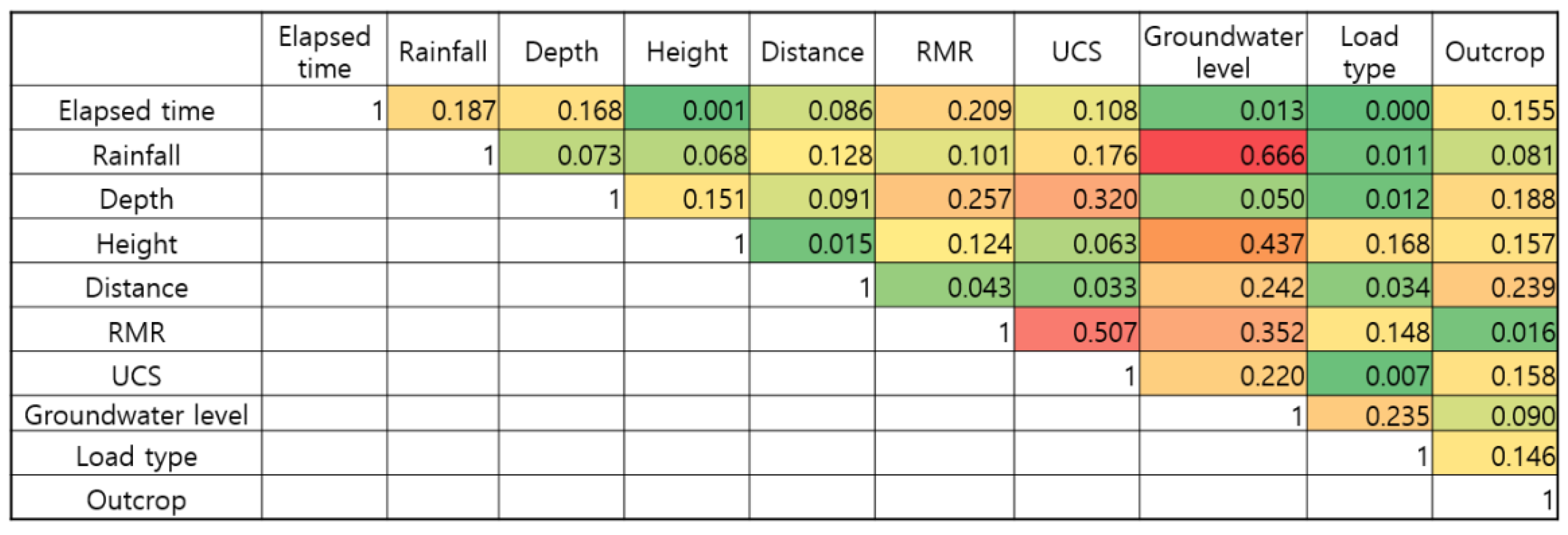
The results showed that the correlation between subsidence occurrence and UCS, or rainfall was very low and that the multicollinearity between RMR and UCS, as well as between groundwater level and rainfall, was high (Figure 6 and Figure 7). These mean that the effects of UCS and rainfall on subsidence are comparatively low, and RMR and groundwater level are closely related to UCS and rainfall respectively. Finally, UCS and rainfall were excluded from the factors for the analyses, and the other nine influence factors were selected, as depicted in Figure 8.

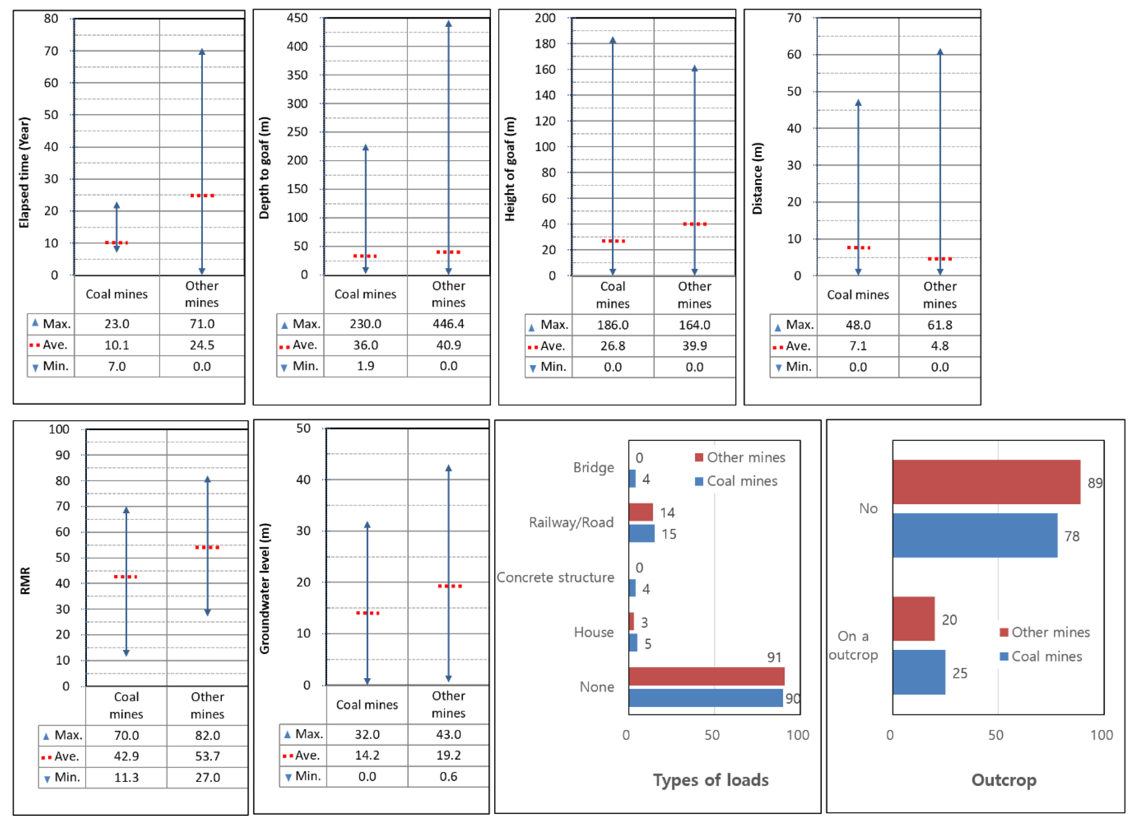
Figure 9 presents the value ranges of the selected data for each factor. The time elapsed from the closing of the mine until an investigation was performed ranged between 7 and 23 years, with an average of 10 years, whereas the time elapsed for the other types of mines ranged between 0 and 71 years, with an average of 25 years. The average depth from ground level to the nearest goaf at a subsidence location was 36 m for coal mines and 41 m for other types of mines. Furthermore, the average horizontal distance was approximately 7 m and 5 m, respectively. The number of investigated locations near a railway or road was 15 and 14, corresponding to about 12% and 13% of the total investigated locations (118 and 108 locations), respectively. The number of locations located on an outcrop was 20 and 25, which corresponds to about 24% and 18% of the total investigated locations, respectively.

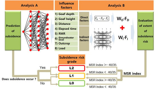
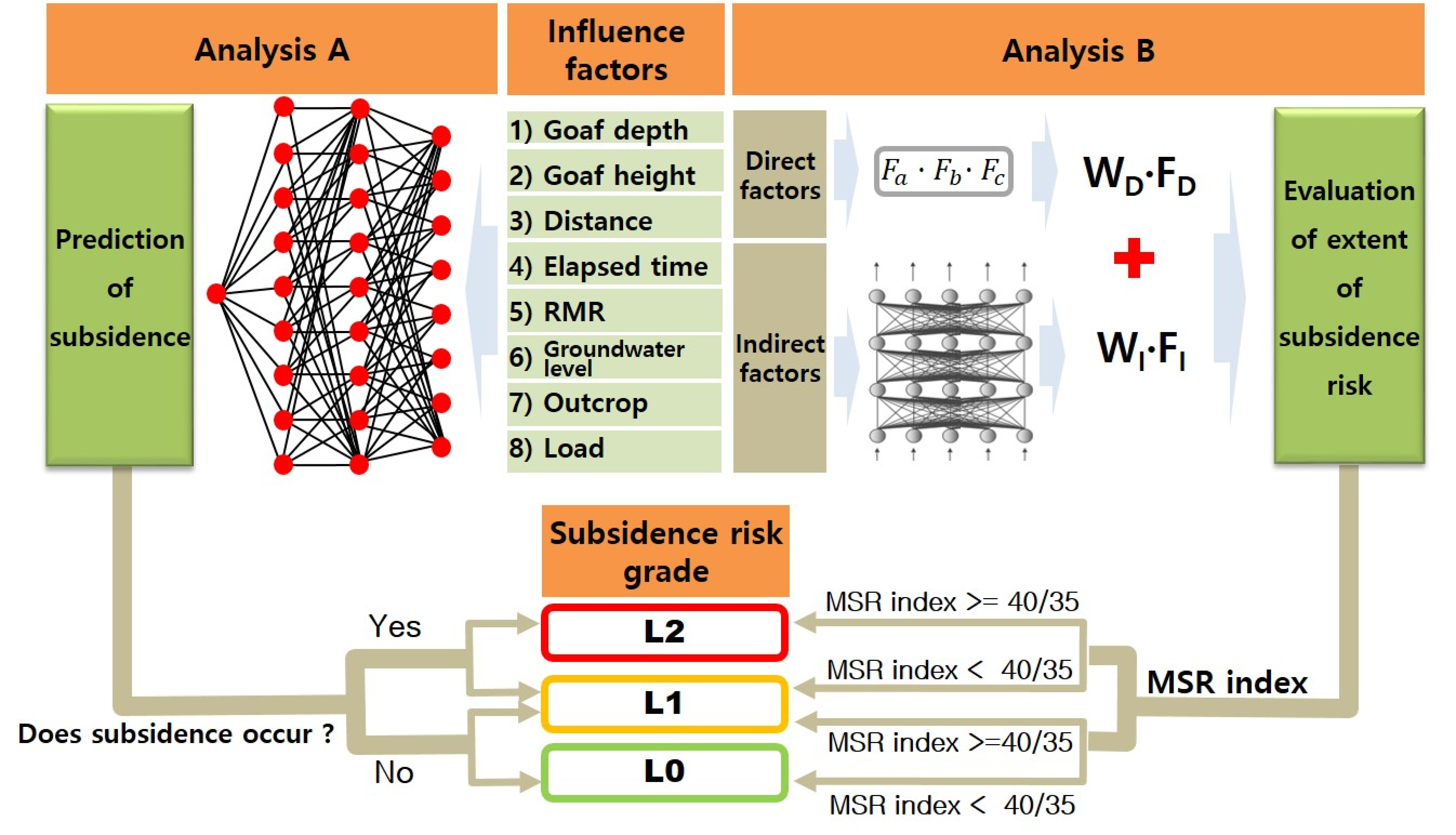
4. Analysis and Discussion

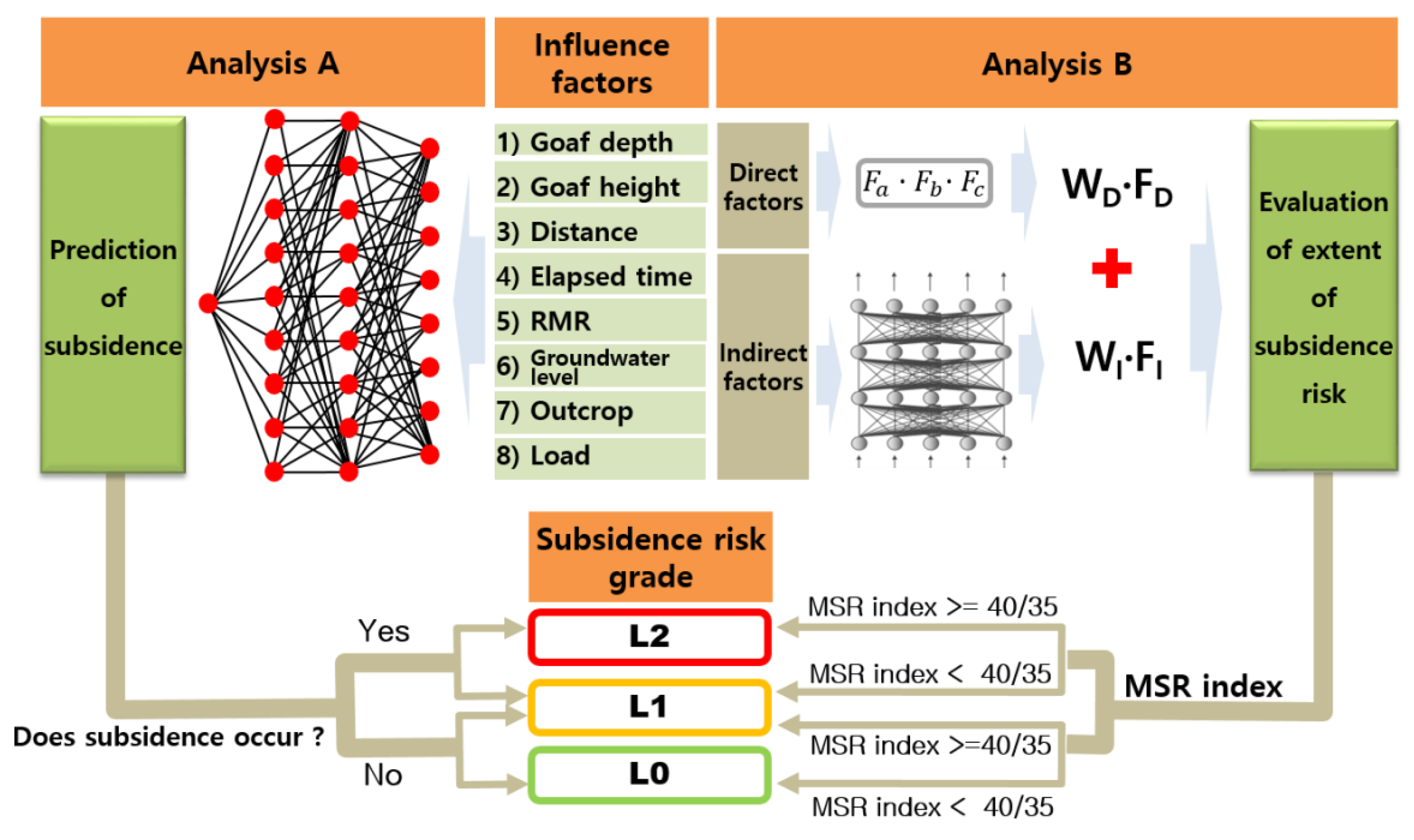
The analysis of this study consisted of two stages: analysis A and analysis B. Analysis A sought to predict whether or not subsidence would occur using an ANN. Analysis B established a mine subsidence risk (MSR) index using an interaction matrix to indicate the extent of risk for subsidence at any given location. The results of both analyses were integrated into a single classification system referred to as the subsidence risk grade, which categorizes the location based on risk level.

4.1. Analysis A

4.1.1. Normalization of the Data

Normalization is a technique often applied as a part of data preparation for machine learning. The goal of normalization is to ensure that every data point has the same scale so that each factor is rated as equally important. Hence, it is only required when features have different ranges. In this study, normalization was used to compare the contribution of each identified influence factor towards the risk of subsidence and was performed by scaling the values of each factor from 0 to 10 points.

4.1.2. Structure of the Model

For optimum learning and prediction of an ANN, the structure of the ANN model and initial conditions in the ANN program need to be established first. Thus, a series of analyses were performed for various cases, varying the number of hidden layers and nodes to determine the optimum structure of the ANN for this study. For this purpose, the same dataset was applied for each case, and the case with minimized error % was adopted as the optimum structure.

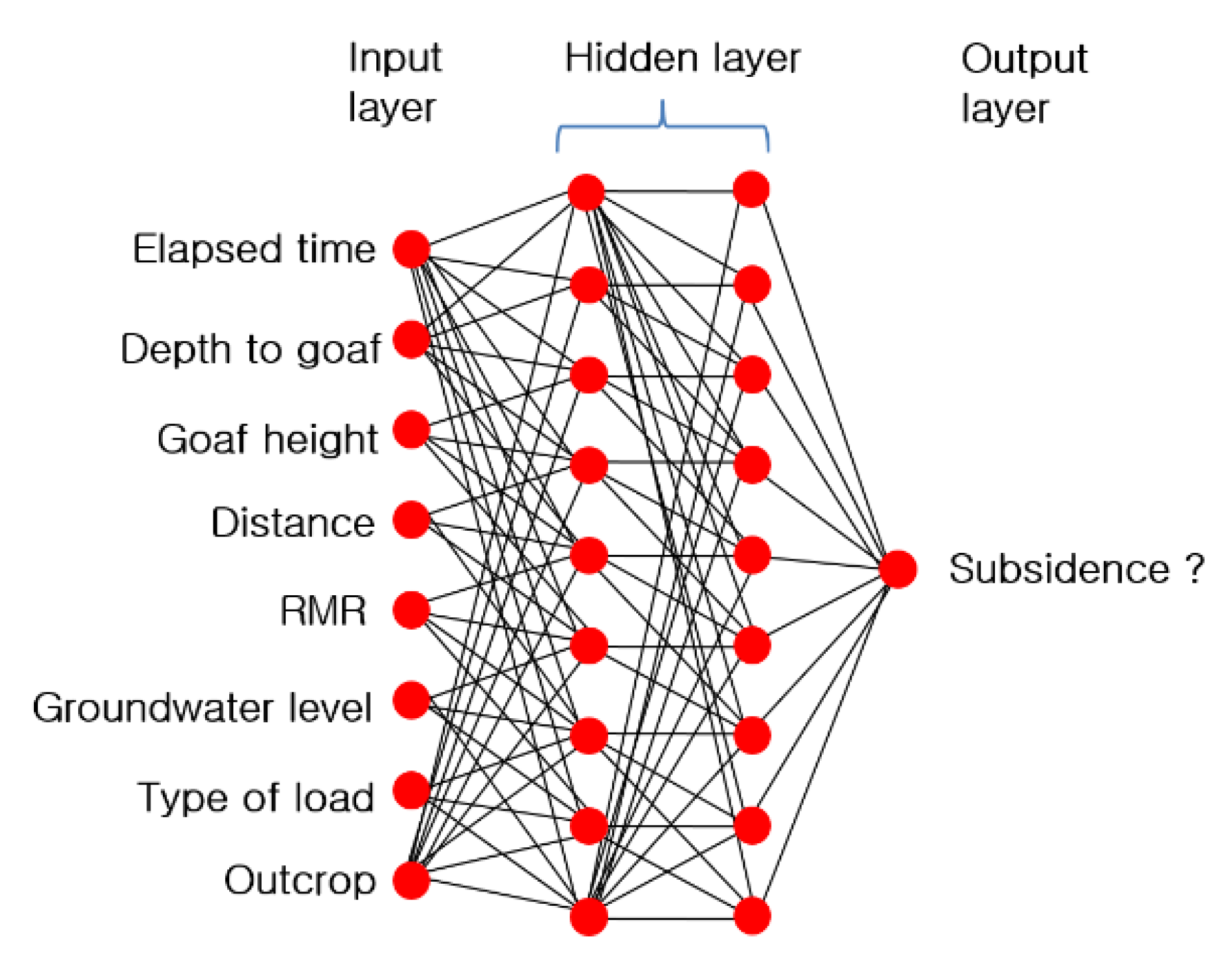
Finally, it was discovered that the optimum structure occurred when the number of nodes for the input, first hidden, second hidden, and output layer was 8, 10, 10, and 1 for coal mines and 8, 9, 9, and 1 for other types of mines, respectively, as depicted in Figure 10.

4.1.3. Setting of the Training Parameters

In the learning and prediction stage of the ANN development, the learning rate in the GDAP program was set to 0.1, and the initial weights were randomly selected between 0.1 and 0.9. As a training algorithm for this analysis, a resilient propagation algorithm that is a variant of the standard back-propagation neural network was used because it leads to much faster training than others and minimizes the error between the predicted output values and the calculated output values. The algorithm propagates the error backwards and iteratively adjusts the weights. The maximum number of iterations and maximum system errors to determine when training should be terminated were set to 20,000 and 0.000001, respectively, applying ‘early stopping’ to avoid overfitting on the training dataset.

4.1.4. Results of Analysis A

After training the model, the accuracy of the model was measured separately for the training datasets (total 207), and validation datasets (total 20) to check for overfitting of the model. The results showed that the accuracies for coal mines for training datasets and validation datasets were 97% and 83%, respectively, and were 97% and 75% for other type mines, respectively, as presented in

Table 2. Accuracy of analysis A by the data type.

Data Type	Accuracy (Number of Data)
	Coal Mines	Other Type Mines
Training data	97%	97%
	(106)	(101)
Validation data	83%	75%
	(12)	(8)

. Logically, because the training was performed using the training datasets, their accuracy was higher than the accuracy for the validation datasets. It is expected that, once additional training datasets are added, in the future, the accuracy for validation will also improve, reducing the overfitting on the training dataset.

4.2. Analysis B

For analysis B, the MSR index was assessed using the eight factors, which were divided into two groups: a direct influence factor group and an indirect influence factor group. The direct influence group consisted of three factors, depth to a goaf, goaf height, and horizontal distance to the nearest goaf, which directly influence subsidence. The indirect influence group included the other five factors: elapsed time, RMR, load type, outcrop, and groundwater level.

4.2.1. Direct Influence Factor Group

Jung et al. [43] suggested a method to evaluate abandoned mine subsidence risk using only the depth to a gangway, which can be collected easily from existing materials. Many other studies also placed much importance on the depth to a gangway or goaf as a major factor inducing subsidence [30,44,45,46,47].

Accordingly, it can be stated that the depth to a goaf is a vital factor to the occurrence of subsidence and that the magnitude of subsidence is greatly affected by goaf height and the horizontal distance to a goaf. Thus, the depth to goaf was classified into 11 groups by using the depth range to allocate the points between 10 and 100, and this was adjusted by goaf height and distance (

Table 3. Points for direct influence factors with their ranges.

Depth (m, Fa)				Points	Height (m, Fb)				Correction Factor	Distance (m, Fc)		Correction Factor
Coal		Other			Coal		Other			Coal and Other
<	1000	<	1000	10	<	1000	<	1000	1.00	<	1000	0.1
<=	60	<=	30	10	<=	27	<=	45	0.95	<=	20	0.1
<=	54	<=	27	20	<=	24	<=	40	0.90	<=	18	0.2
<=	48	<=	24	30	<=	21	<=	35	0.85	<=	16	0.3
<=	42	<=	21	40	<=	18	<=	30	0.80	<=	14	0.4
<=	36	<=	18	50	<=	15	<=	25	0.75	<=	12	0.5
<=	30	<=	15	60	<=	12	<=	20	0.70	<=	10	0.6
<=	24	<=	12	70	<=	9	<=	15	0.65	<=	8	0.7
<=	18	<=	9	80	<=	6	<=	10	0.60	<=	6	0.8
<=	12	<=	6	90	<=	3	<=	5	0.55	<=	4	0.9
<=	6	<=	3	100	=	0	<=	0	0.00	<=	2	1.0

). Finally, the subsidence risk for direct influence factors was calculated by Equation (1).

$$F_D=F_a·F_b·F_c$$

(1)

4.2.2. Indirect Influence Factor Group

An interaction matrix is a tool used to represent correlations among multiple components simultaneously. The given components are aligned horizontally in the matrix so that their correlations are expressed in parallel links rather than in one-to-one relations. The approach is based on the concept that every factor of an actual location is related to every other factor, albeit to varying degrees [48].

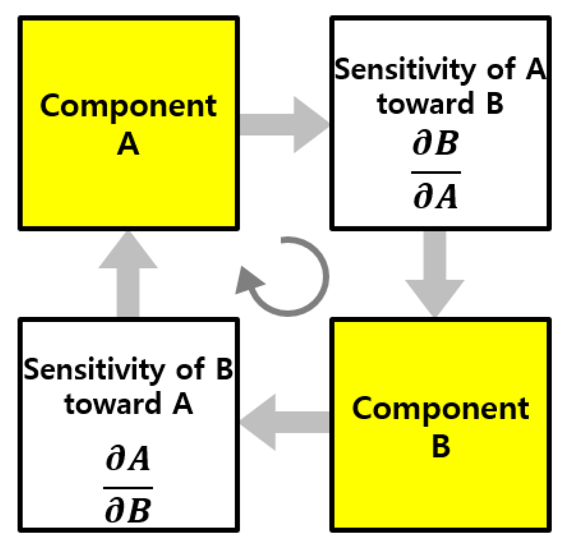
Hudson [49] positioned subject components as diagonal entries and represented their interactions in the clockwise direction. As shown in Figure 11, the major components A and B are placed as diagonal entries, and the components are linked in the clockwise direction. Accordingly, the components to the right of A and above B represent the sensitivity of A toward B. Conversely, the components to the left of B and below A represent the sensitivity of B toward A. The significance of each component of the matrix can be expressed with partial derivatives. Although interactions can be represented with the matrix in a simple manner, the critical question is how the sensitivity of each component should be determined for best use of the concept for analysis and application of field data [49,50]. Although only two factors were used to explain the concept in Figure 11, the interaction matrix can be constructed for multiple factors based on the identical concept. Although the matrix is mathematically capable of expressing the correlations among all the factors in diagonal entries, during the initial stage, Hudson [49] constructed each component of the matrix, indicating sensitivity by independently considering the linear relationship between linked components (A and B in Figure 11) and intuitively assigning values to the matrix.

Based on the concept that two or more components on the matrix diagonal are related to each other with varying degrees of influence, Jiao and Hudson [51] proposed an algorithm for constructing an interaction matrix for which all of the component values of the matrix are fully coupled. However, each component of the interaction matrix is still determined based on the intuition of experts, making its objective assessment difficult. Yang and Zhang [50] proposed constructing an interaction matrix by using the ANN. To do so, they introduced the concept of the relative strength effect (RES) and an ANN-based calculation algorithm to assess the linkage strength among the components. For this study, a RES value between 0 and 1 was used to represent the mutual relationship between components.

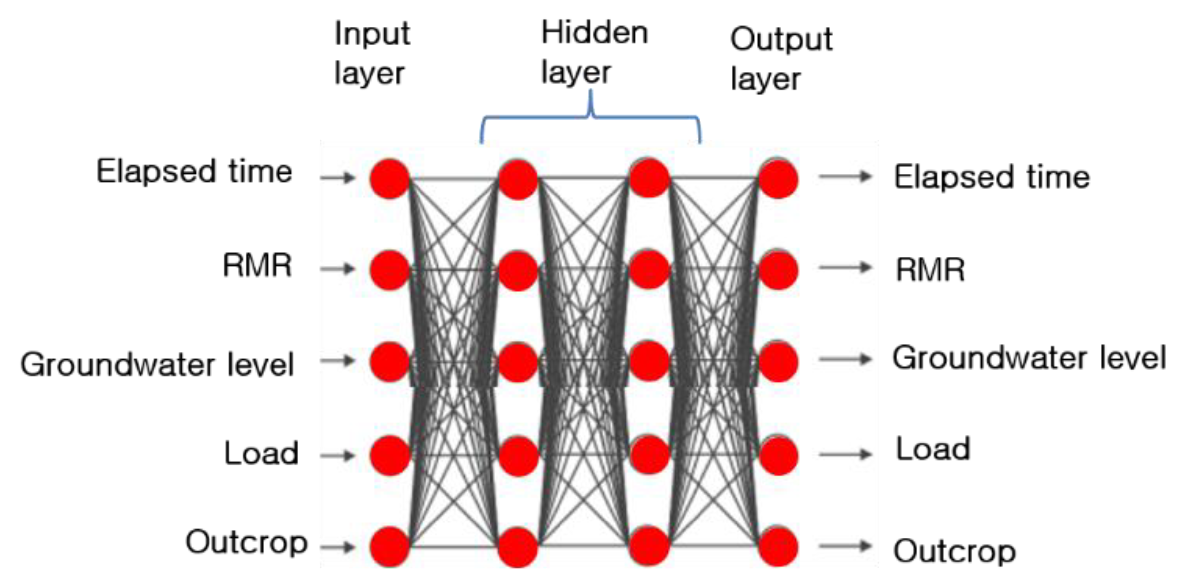
Figure 12 shows the architecture of the ANN specially organized for sensitivity analysis, which consists of the same number of nodes for one input layer, one output layer, and two hidden layers.

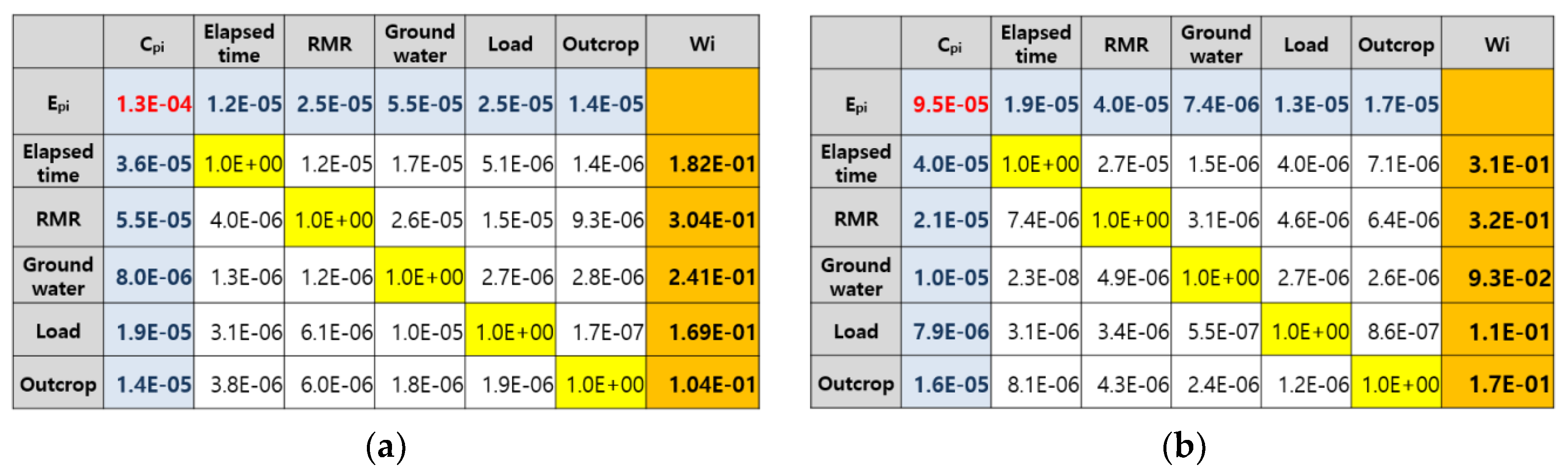
Once training is complete, a partial derivative of an input node can be calculated for each output node using the ANN sensitivity analytical system [39]. All five components of the interaction matrix can then be assigned with the calculated partial derivatives. Figure 13 shows an interaction matrix constructed using this process. Every value on the diagonal calculated by the trained ANN is 1.0, which is natural because, in theory, a partial derivative of an identical component should always be 1.0.

According to the basic concept of the applied interaction matrix, the row of the subject factor represents the causes it has on other factors, and the sum of the rows of the matrix indicates its causes on the entire system. Similarly, the column of the factor represents the influence of other factors, corresponding to the effects. The sum of the columns, therefore, represents the effects on the entire system [49,52]. Based on these concepts, a representative value can be assessed to express the degree of influence of each selected factor on the location. The representative value is calculated as follows.

First, the rows and columns of the interaction matrix are added so that each factor represents the cause and effect of the influence on the entire system. The degree of influence of each factor (i) on the entire system as a cause is denoted by C_pi, and as an effect by E_pi. In Figure 13, C_pi is indicated on the right of each row heading and E_pi is indicated below each column heading. The two categories can be expressed as Equation (2)

$$\begin{gathered} C_{pi}={{\displaystyle \sum }}_{n=1}^{n_{max}}\left(I_{mn}\right), m=i \\ {E}_{pi}={\displaystyle \sum }_{m=1}^{m_{max}}\left(I_{mn}\right), n=i \end{gathered}$$

(2)

where I_mn represents each component of the m × n interaction matrix, n_max represents the total number of columns, and m_max represents the total number of rows.

Consequently, the interaction matrix must be able to comprehensively express the links among the influence factors of the given location related to subsidence. The influence weights assigned to each factor are expressed as a percentage of the sum of the system’s cause (C_pi) and effect (E_pi) according to the following equation. The total sums of causes and effects are expressed as Equation (3)

$$W_i=\frac{\left(C_{pi}+E_{pi}\right)}{({{\displaystyle \sum }}^{}{C}_{pi}+{{\displaystyle \sum }}^{}{P}_{pi})}\times \frac{100}{N_{grade}}$$

(3)

where N_grade is the number of grades assigned to the factor i.

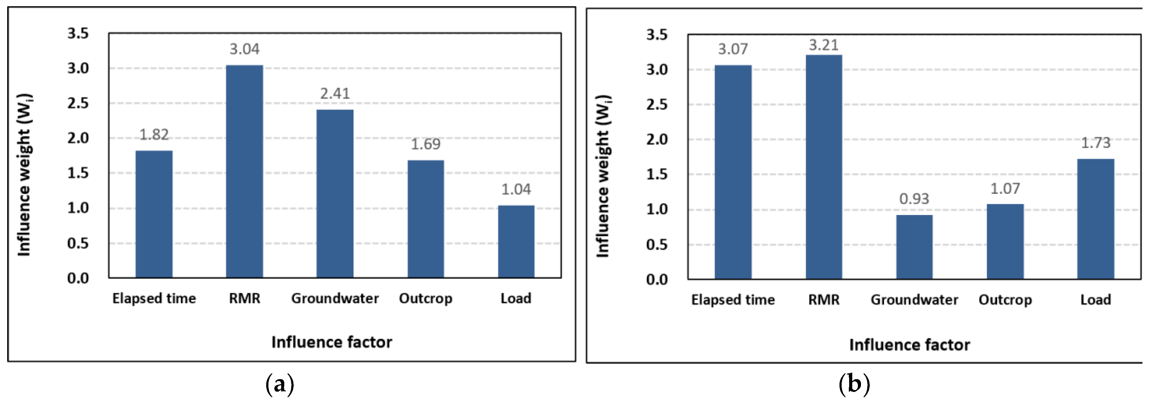
Figure 14 provides the influence weights for the five influence factors calculated from Equation 3. The results show that the most sensitive factor affecting the subsidence for both types of mines was RMR, while the load type and groundwater level were least sensitive for subsidence for coal mines and other types of mines, respectively.

Accordingly, the subsidence risk for indirect influence factors can be defined as

$$\mathrm{Subsidence}\mathrm{risk}\mathrm{for}\mathrm{indirect}\mathrm{factors}\left(F_I\right)={{\displaystyle \sum }}^{}{W}_i·V_i$$

(4)

where V_i denotes the normalized value for each factor i at the location in question, as indicated in Section 4.1.1. The final possible F_I ranges from 0 to 100.

4.2.3. Mine Subsidence Risk Index

The mine subsidence risk (MSR) index is defined as in Equation 5 by combining the two subsidence risks by the direct influence group and the indirect influence group.

MSR index = W_D·F_D + W_I·F_I

(5)

Here, W_D and W_I are the weights of subsidence risk for the direct influence factor group and the indirect group, respectively. The two weights can be determined by a series of sensitivity analyses on subsidence for the direct group and the indirect group.

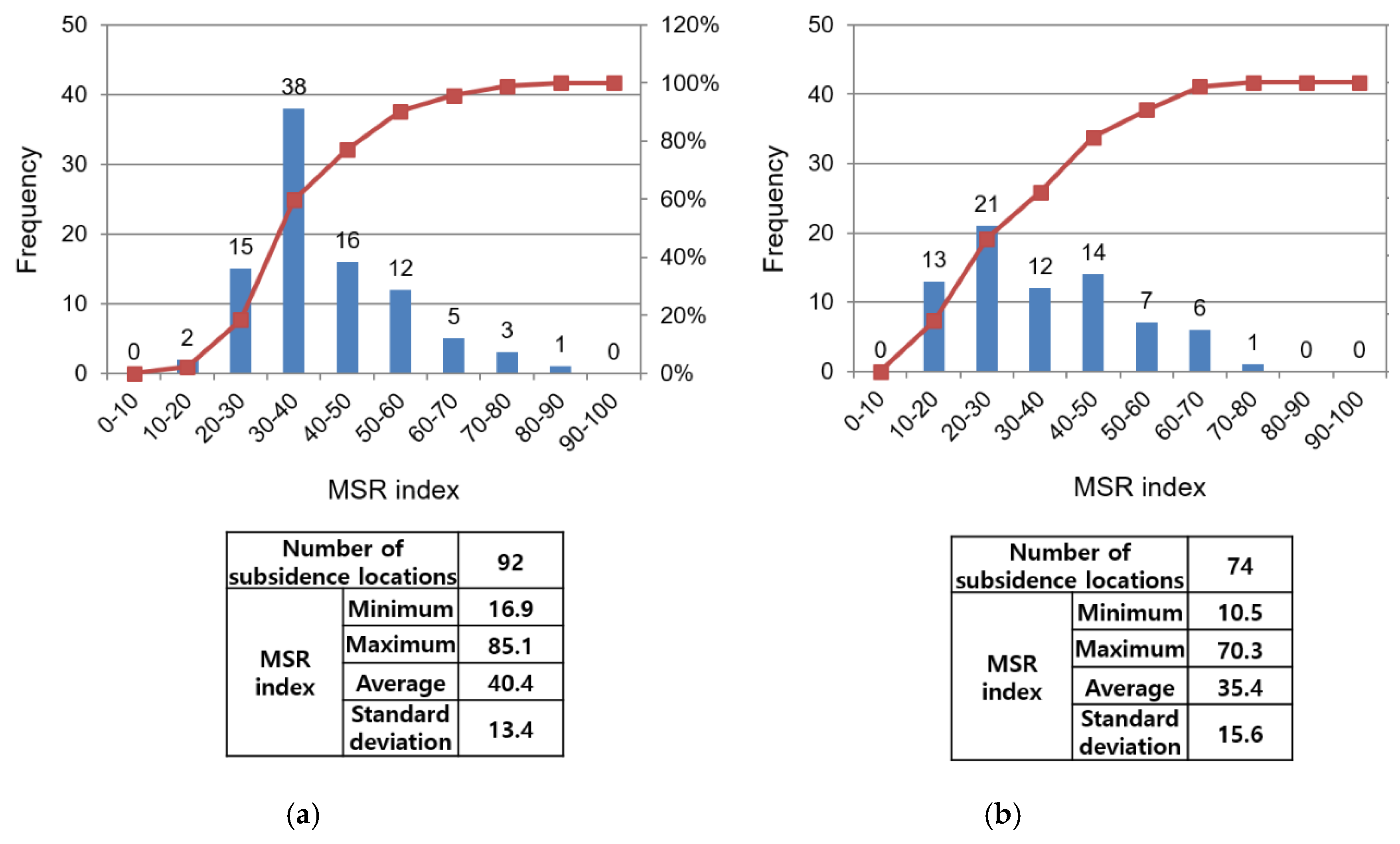
Finally, the MSR index is defined as in Equations (6) and (7), and the final MSR index for all of the subsidence locations is summarized as Figure 15. A higher MSR index implies a higher possibility of subsidence.

MSR index for coal mines = 0.5·F_D + 0.5·F_I

(6)

MSR index for other types of mines = 0.65·F_D + 0.35·F_I

(7)

4.3. Mine Subsidence Grade

Analysis A is used to predict whether subsidence can occur for the given factors, but it always includes the possibility of incorrect prediction as well. Analysis B is necessary to back up the results of analysis A by assessing the MSR index to indicate the extent of risk for subsidence at the location in question.

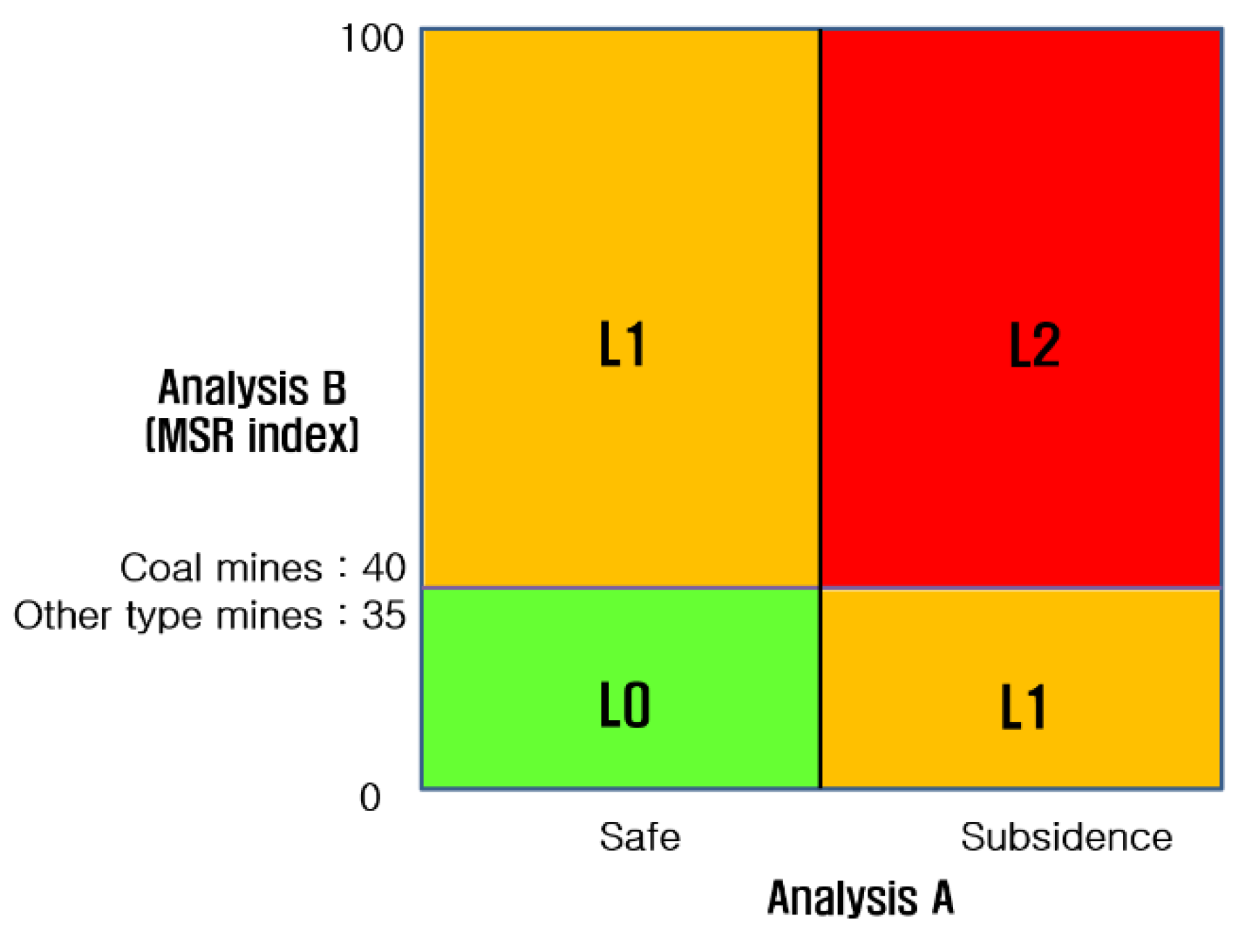
Finally, in this study, the grade of MSR was classified into the three categories, level 0 (L0, low risk), level 1 (L1, moderate risk), and level 2 (L2, high risk), by combining the results of analyses A and B, as indicated in Figure 16. In this diagram, the MSR index for deciding L0 or L1 is determined considering the average values of the MSR index presented in Figure 15.

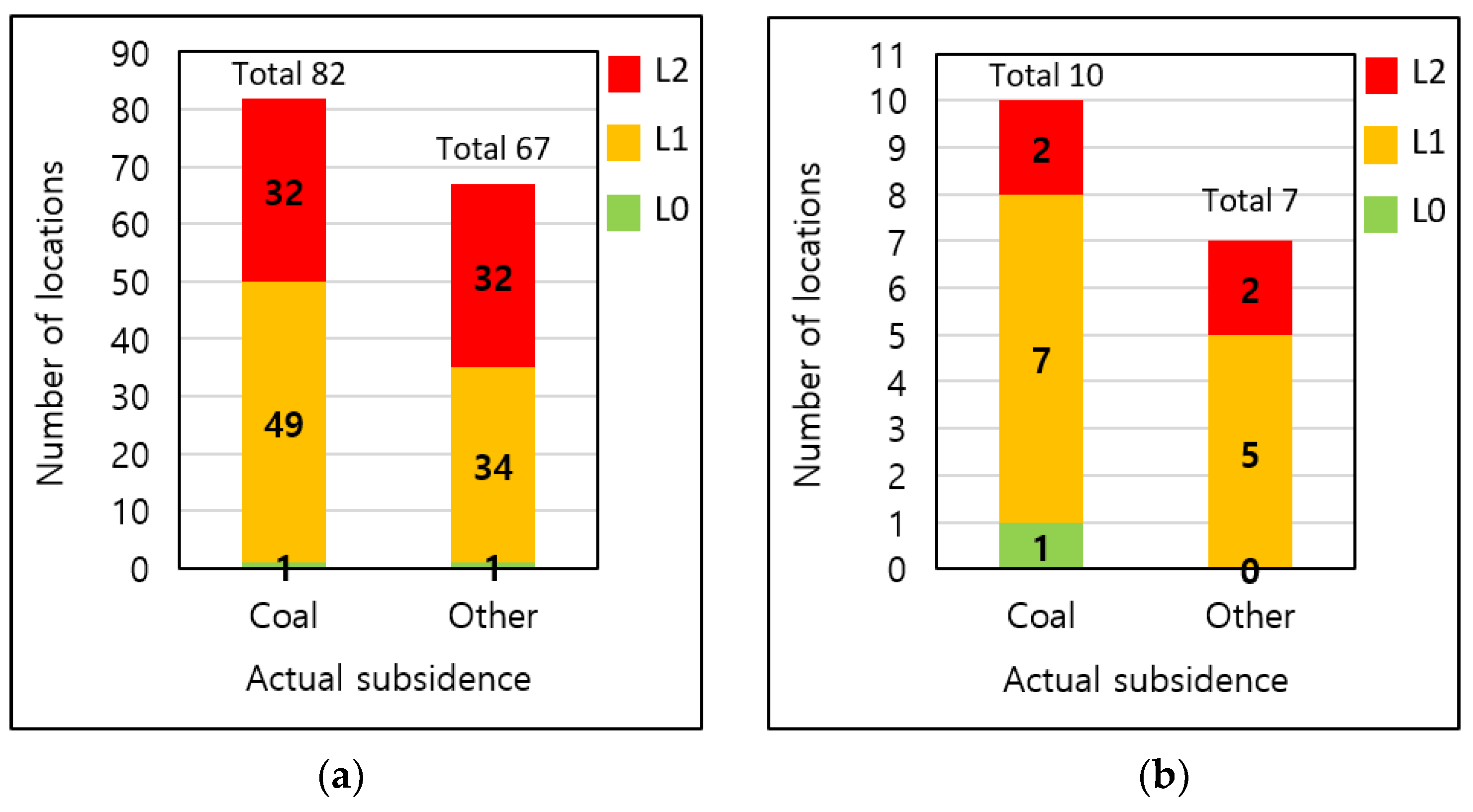
The subsidence risk grades determined by the diagram for the training data and the validation data are presented in Figure 17. For the training data of coal mines, only one of the 82 locations where subsidence actually occurred was predicted to be safe, which means that the correct prediction percentage for the training data is 98.8% (=81/82 subsidence locations). For the other types of mines, the correct prediction percentage was 98.5% (=66/67 subsidence locations). For the validation data, the correct prediction percentage was 90% (=9/10 subsidence locations) and 100% (=7/7 subsidence locations) for the coal mines and the other types of mines, respectively.

The overall procedure for deciding subsidence risk grade is summarized in Figure 18.

5. Testing the Model Using New Data

The applicability of the subsidence risk grade was tested with newly collected 22 subsidence data from five abandoned mines. The data consist of 12 locations (6 subsidence and 6 no subsidence locations) at 3 coal mines and 10 locations (7 subsidence and 3 no subsidence locations) at 2 other types of mines. The information of data is summarized in

Table 4. New subsidence data.

Type	Mine Name	No.	Subsidence	Elapsed Time 1 (Year)	RMR	Groundwater Level (m)	Outcrop	Load Type 2	Depth 3 (m)	Height 4 (m)	Distance 5 (m)
Coal	CM1	1	Yes	15	25	18	Yes	0	3	16	0
		2	Yes	15	20	13	Yes	1	2	20	0
		3	Yes	19	16	10	No	0	6	13	0
		4	No	19	26	25	No	0	7	13	3
		5	No	19	32	29	No	0	15	8	8
	CM2	1	Yes	26	22	27	Yes	3	14	2	0
		2	Yes	26	21	31	No	3	30	2	42
		3	No	26	17	20	No	0	30	2	126
		4	No	26	20	25	No	0	35	1	126
	CM3	1	Yes	24	33	20	Yes	3	19	13	9
		2	No	24	26	22	No	3	32	16	44
		3	No	24	26	26	No	3	38	11	55
Other types	OM1	1	Yes	39	53	4	No	3	3	2	14
		2	Yes	39	53	2	No	3	1	2	5
		3	No	39	37	4	No	0	3	2	22
		4	No	39	37	5	No	0	10	2	32
	OM2	1	Yes	31	64	12	No	0	33	5	5
		2	Yes	31	30	1	No	4	1	16	1
		3	Yes	31	40	4	No	3	4	11	2
		4	Yes	31	50	7	No	2	7	6	3
		5	Yes	31	60	10	No	1	10	1	4
		6	No	31	42	7	No	0	27	5	7

¹ Elapsed time: The time elapsed since the corresponding abandoned mine was closed. ² Load type: 0 (none), 1 (house), 2 (concrete structure), 3 (railway/road), 4 (bridge). ³ Depth: The depth to goaf crown. ⁴ Height: The height of the goaf beneath the corresponding subsidence. ⁵ Distance: The distance from the nearest underground goaf to the ground location to be investigated.

.

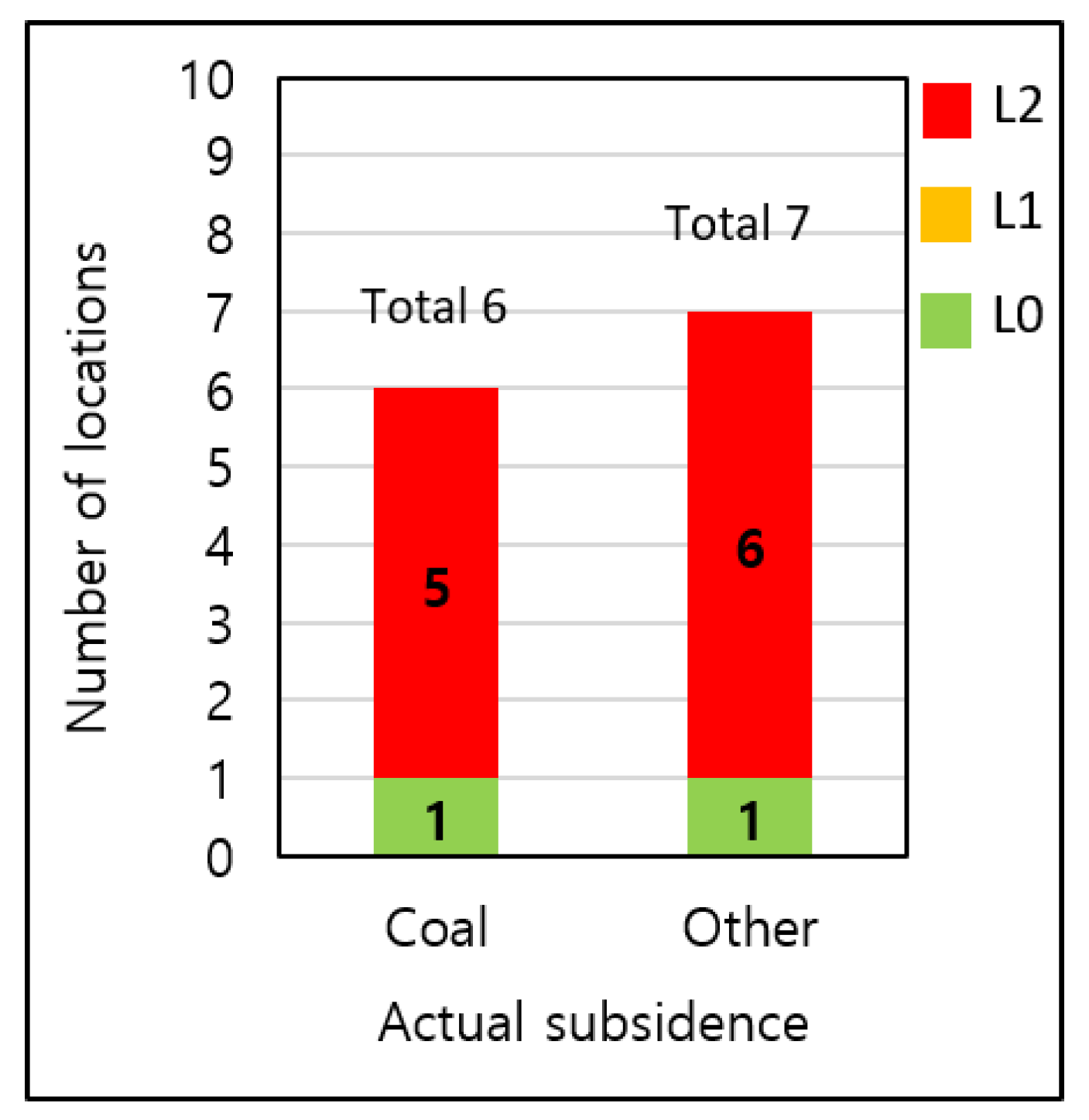
The subsidence risk grade analyses were carried out through the procedure illustrated in Figure 19. The results showed that five of six coal mine locations where subsidence had occurred were predicted to be L2 and that six of the seven locations for other types of mines were predicted as L2. For both types of mines, no location was predicted to be L1. Finally, it was found that the correct prediction percentage was 83% (5/6 subsidence locations) for coal mines and 86% (6/7 subsidence locations) for the other types of mines.

It is thought that the main reason for the lower correct prediction percentage for the new data than the data for training was that the number of newly investigated locations was much smaller than the that for the training data.

Finally, the results imply that the subsidence risk grade model could generally be used to assess the subsidence risk for an abandoned mine. Nevertheless, much more subsidence data with greater variations in ground conditions will be essential and various types of analyses by numerical and empirical approaches, etc. need to be combined to improve the correct prediction percentage of subsidence.

Meanwhile, this analysis process can be used as an initial method screening the specific locations that are at high risk of subsidence, for subsequent detailed analyses by other approaches, for example, the amplitude or rate of the subsidence at high risk can be calculated by empirical methods, methods employing influence functions, and/or methods employing theoretical models [32].

6. Conclusions

This paper establishes a mine subsidence risk index and a subsidence risk grade based on two separate analyses using ANN to predict whether subsidence can occur at a ground location of an abandoned mine. The primary conclusions of the study are summarized below:

(1) From a total of 467 investigated locations in this study, 227 locations from 37 abandoned mines were selected for analysis. Among these, 118 locations were from 15 abandoned coal mines, and 109 locations were from other types of mines (i.e., gold, silver, metal). The numbers of locations where subsidence had and had not occurred were 166 and 61, respectively.

(2) The correlation and multicollinearity analyses among 10 factors related to mine subsidence were performed to improve the prediction accuracy. The results showed that the correlation between subsidence occurrence and UCS, or rainfall was very low and that the multicollinearity between RMR and UCS as well as between groundwater level and rainfall was high. This means that the effects of UCS and rainfall on subsidence are comparatively low, and RMR and groundwater level are closely related to UCS and rainfall respectively. Finally, eight factors excluding UCS and rainfall (i.e., elapsed time, depth to goaf, goaf height, distance to the nearest goaf, RMR (rock mass rating), groundwater level, load types on the investigated location, and the existence of an outcrop on the investigated location) were selected.

(3) The analysis consisted of two separate stages, analysis A and analysis B. Analysis A was conducted to predict whether subsidence could occur using an ANN model of machine learning. Analysis B involved assessing the mine subsidence risk index to indicate the extent of risk for subsidence at the location. After training the model in analysis A, the results showed that the correct prediction percentages for the validation datasets of coal mines and other types of mines were 83% and 75%, respectively.

In analysis B, the eight factors were divided into two groups, a direct influence factor group (depth to a goaf, goaf height, and horizontal distance to the nearest goaf) and an indirect influence factor group (elapsed time, RMR, load type, outcrop, and groundwater level), to assess the mine subsidence risk (MSR) index.

The final determination of subsidence possibility is made using a subsidence risk grade that is established based on the two analyses. The analysis results showed that the correct prediction percentage was 90% (=9/10 subsidence locations) for the 10 validation data of coal mines and 100% (=7/7 subsidence locations) for the 7 validation data of other types of mines.

(4) To verify the prediction model, new datasets for 22 locations—including 9 locations with no subsidence—were selected from 5 abandoned mines and investigated. The correct prediction percentage for coal mines was 83% (=5/6 subsidence locations), and the correct prediction percentage for other types of mines was 86% (=6/7 subsidence locations).

Although this model performed reasonably well in the assessment of potential subsidence at various locations, the sample size was relatively small; thus, additional analyses should be performed at other mine locations and in a larger variety of ground conditions to more clearly verify the model.

(5) It is thought that more reliable results can be obtained when various types of analyses by numerical, statistical, and theoretical approaches are combined. This study can be used as an initial method for screening the specific locations that are at high risk of subsidence and thus require immediate additional investigation, from an extensive mine area for subsequent detailed analyses by the other approaches.