Data Sampling Methods to Deal With the Big Data Multi-Class Imbalance Problem

Abstract

The class imbalance problem has been a hot topic in the machine learning community in recent years. Nowadays, in the time of big data and deep learning, this problem remains in force. Much work has been performed to deal to the class imbalance problem, the random sampling methods (over and under sampling) being the most widely employed approaches. Moreover, sophisticated sampling methods have been developed, including the Synthetic Minority Over-sampling Technique (SMOTE), and also they have been combined with cleaning techniques such as Editing Nearest Neighbor or Tomek’s Links (SMOTE+ENN and SMOTE+TL, respectively). In the big data context, it is noticeable that the class imbalance problem has been addressed by adaptation of traditional techniques, relatively ignoring intelligent approaches. Thus, the capabilities and possibilities of heuristic sampling methods on deep learning neural networks in big data domain are analyzed in this work, and the cleaning strategies are particularly analyzed. This study is developed on big data, multi-class imbalanced datasets obtained from hyper-spectral remote sensing images. The effectiveness of a hybrid approach on these datasets is analyzed, in which the dataset is cleaned by SMOTE followed by the training of an Artificial Neural Network (ANN) with those data, while the neural network output noise is processed with ENN to eliminate output noise; after that, the ANN is trained again with the resultant dataset. Obtained results suggest that best classification outcome is achieved when the cleaning strategies are applied on an ANN output instead of input feature space only. Consequently, the need to consider the classifier’s nature when the classical class imbalance approaches are adapted in deep learning and big data scenarios is clear.

1. Introduction

The huge amount of data continuously generated by digital applications is an important challenge for the machine learning field [1]. This phenomena is not only characterized by the volume of information, but also by the speed of transference and the variety of data; i.e., the big data characteristics [2,3]. Concerning to the volume of information, a dataset belongs to big data scale when it is difficult to process with traditional analytical systems [4].

In order to efficiently seize the large amount of information from big data applications, deep learning techniques have become an attractive alternative, because these algorithms generally allow to obtain better results than traditional machine learning methods [5,6]. Multi-Layer Perceptron (MLP), the most common neural network topology, has been also translated to the deep learning context [7]. Deep Learning MLP (DL-MLP) incorporates two or more hidden layers in its architecture [8], which increases the computational cost of processing large size and high dimension datasets. Nevertheless, this disadvantage can be overtaken by using modern efficient frameworks, such as Apache-Spark [9] or Tensor-Flow [10]. Thus, the high performance, robustness to overfitting, and high processing capability of these deep neural networks can be exploited.

Machine learning and deep learning algorithms are strongly affected by the class imbalance problem [11,12,13,14,15]. The latter refers to some difficulties that appear when the number of samples in one or more classes in the dataset is fewer than another class (or classes), thereby producing an important deterioration of the classifier performance [16]. In the literature, many studies dealing with this problem have been reported [17]; in particular, the data sampling methods such as Random Over-Sampling (ROS), which replicate samples from the minority class, and Random Under-Sampling (RUS), which eliminate samples from the majority class. These methods bias the discrimination process to compensate the class imbalance ratio [18].

Data sampling methods have important drawbacks, such as longer training times and over-fitting, which are more likely to occur when minority samples are replicated. Additionally, the loss of information is common when many samples are removed from majority classes, potentially dismissing useful information for the classifier [19,20,21]. Then, more "intelligent" sampling, methods including a heuristic mechanism, have been developed [17,22,23].

Synthetic Minority Over-sampling Technique (SMOTE) is a heuristic over-sampling algorithm. It generates artificial samples from the minority class by interpolating existing instances that lie close together. Nowadays, it is one the most popular data sampling methods [1] and it has motivated the development of other over-samplings algorithms [24]. Similarly, under-sampling methods have been incorporate a heuristic component [25], some of the most outstanding examples being the Tomek’s Links (TL) [26], Editing Nearest Neighbor (ENN) [27], and Condensed Nearest Neighbor rule (CNN) [28], among others [22,29,30,31,32,33].

Another way to deal with the class imbalance problem has been through the Cost Sensitive (CS) approach [34], which has become an important topic in deep learning research in recent years [13,14,15,35]. CS considers the costs associated with misclassifying samples; i.e., it uses different cost matrices describing the costs of misclassifying any particular data sample [29]. The over and under-sampling could be a special case of CS techniques [34,36].

In neural networks, CS can be performed on several ways [37]: (a) cost-sensitive classification, where the learning process is not modified and only the output probability estimates for the network are adjusted during the testing stage; (b) adapting the output of the network, unlike the last one, the neural network output is appropriately scaled; (c) adapting the learning rate, meaning to include a constant factor that modify the learning rate value; (d) minimization of the misclassification costs or loss function (in deep learning), where the loss function is corrected by introducing the factor that compensates the classification errors or the class imbalance.

Reference [11] presents a novel focal loss to deal with the class imbalance problem on dense object detection. It can be seen as a CS approach which applies a modulating term (weighting factor) to the cross entropy loss in order to focus learning on hard negative examples and addressing the class imbalance. The weighting factor can be set by inverse class frequency or treated as a hyper-parameter to be set by cross validation. Reference [13] proposes a cost-sensitive deep neural network which can automatically learn (during training) robust feature representations for both the majority and minority classes.

Ensemble learning is an effective method that combines multiple classifiers and class imbalance approaches to improve the classification performance on several applications [31,38,39,40]. Reference [41] proposes a solution for breast cancer diagnosis: to use decision trees and Multi-Layer Perceptrons as base classifiers in order to build an ensemble similar to the Easy Ensemble algorithm, and sub-sampling methods to deal with the class imbalance problem. In [42], an ensemble of support vector machines is used, where the maximum margin is adopted to guide the ensemble learning procedure for multi-class imbalance classification. In [14], a hybrid optimal ensemble classifier framework that combines under-sampling and cost sensitive methods is proposed.

The combination of deep learning and an ensemble classifier has been performed. For example, in [43], a software bug prediction is presented. It has two stages: deep learning (auto-encoder) and ensemble learning, and it was noticed to be able to deal with the class imbalance and over-fitting problem. In big data scenarios, the conjunction of ensembles and clustering methods has been proposed, as was demonstrated by [44], where ensembles with datasets preprocessed by clustering and sampling methods were built. Moreover, the use of clustering and sampling techniques to deal with the class imbalance problem has been increased [45,46,47]. In the machine learning context, extensive and comprehensive reviews about of ensembles and class imbalance problem have been performed [30,38,39].

It has seen that big data class imbalance approaches have been addressed by adaptation of traditional techniques, mainly sampling methods [21,44]. However, recent studies show that some conclusions from machine learning are not applicable to the big data context; for example, in machine learning is common that SMOTE performs better than ROS [24], but in big data some results do not show this trend [1,48]. In addition, only a few works have been addressed to deal with the class imbalance in big data by using “intelligent” or heuristic sampling techniques [17,49]. Thus, more studies are need in order to test methods that traditionally present good performances in machine learning (such as the random and heuristic sampling algorithms) at the big data scale.

The potential of traditional sampling methods on deep learning neural networks in the big data context is studied in this work. The main contributions of this research are: (a) This paper is focused in dealing with multi-class imbalance problems, which have hardly been investigated [50,51,52] and they are critical issues in the field of data classification [45,53]. (b) It addresses one of the most popular deep learning methods (Artificial Neural Networks, ANN), a specialized research topic, with details on some particular aspects of the classifier, such as answering the question: Is it pertinent to use methods that work in the features space of ANN classifiers that set the decision boundary in the hidden space? (c) Results that notice the effectiveness of applying editing methods on the output neural network in order to improve the deep neural network classification performance are presented.

2. Deep Learning Multi-Layer Perceptron

The Multi-Layer Perceptron (MLP) constitutes the most conventional Artificial Neural Network (ANN) architecture [54]. It is formed by a set of simple elements called computational nodes or neurons, where each node sends a signal that depends on its activation state [55]. Before arriving at the receiver neuron, the output is modified multiplying it by the corresponding weight of the link. The signals ($net$) are accumulated in the receiver node and the neurons are grouped forming layers. MLP is commonly based on three layers: input, output and one hidden layer [7]. The MLP has been translated into a deep neural network by incorporating two or more hidden layers within its architecture, making it a Deep Learning MLP (DL-MLP). This allows it to reduce the number of nodes per layer and it uses fewer parameters, but it also leads to a more complex optimization problem [8]; however, due to the availability of more efficient frameworks, such as Apache-Spark and Tensorflow, this disadvantage is less restrictive than before.

MLP is a practical vehicle with which to perform a nonlinear input-output mapping of a general nature [56]. Given a set of input vectors x and a set of wished answers d, learning systems must find parameters linking these specifications. The j output of an ANN: $y_j=\widehat{f}(\mathbf{x},\mathbf{w})$ depends on a set of parameters $\mathbf{w}$ (weights), which can be modified to minimize the discrepancy between the system output z and the answer desired d. The aim of a MLP is to represent the behavior of $\widehat{f}(\mathbf{x},\mathbf{w})$, in a region R of the input space, by means of a linear combination of functions ${\phi }_j\left(\mathbf{x}\right)$ as follows:

$$\widehat{f}(\mathbf{x},\mathbf{W})=\sum _{h=1}{w}_{kh}^L{\phi }_h^{(L-1)}\left(\mathbf{x}\right),$$

(1)

$${\phi }^{(L-1)}\left(\mathbf{x}\right)=\sum _{h=1}{w}_h^{(L-1)}{\phi }_h^{(L-2)}\left(s_i\right),$$

(2)

$$s_i=\sum _h{w}_{hi}^l{\phi }_h^{(l-1)}\left(s_{(i-1)}\right).$$

(3)

If $l=1$ then $s_i={\sum }_h{w}_{hi}{x}_h$; i.e., $s_i$ is the i-th input hidden neuron on the first hidden layer; $w_i^l$ is the weight connected to the i-th input of the h hidden neuron on the l-th hidden layer with $(l-1)$-th hidden layer; and ${\phi }_h^{l-1}$ is the h-th hidden node output on the $(l-1)$-th hidden layer. L is the total number of hidden layers.

Traditionally, MLP has been trained with the back-propagation algorithm (which is based in the stochastic gradient descent) and its weights randomly initialized [54,57]. However, in the latest versions of DL-MLPs, the hidden layers are pretrained by an unsupervised algorithm and the weights are optimized by the back-propagation algorithm [7]. MLP uses sigmoid activation functions, such as the hyperbolic tangent or logistic function. In contrast, DL-MLP includes (commonly) the Rectified Linear Unit (ReLU) $f\left(z\right)$= max $(0,z)$ because it typically learns much faster in networks with many layers, allowing the training of a DL-MLP without unsupervised pretraining.

There are three variants of the descending gradient that differ in how many data are used to process the gradient of the objective function [58]: (a) batch gradient descent calculates the gradient of the cost function to the parameters for the entire training dataset, (b) stochastic gradient descent performs an update of parameters for each training example and (c) mini-batch gradient descent takes the best of the previous two and performs the update for each mini-batch of a given a number of training examples. The most common algorithms of descending gradient optimization are: (a) Adagrad, which adapts the learning reason of the parameters, making bigger updates for less frequent parameters and smaller for the most frequent ones; (b) Adadelta—an extension of Adagrad that seeks to reduce aggressiveness, monotonously decreasing the learning rate instead of accumulating all the previous descending gradients, restricting accumulation to a fixed size; and (c) Adam, which calculates adaptations of the learning rate for each parameter and stores an exponentially decreasing average of past gradients [59]. Other important algorithms are AdaMax, Nadam and RMSprop [58].

In general terms, training methods intends to minimize the error between $f\left(\mathbf{w}\right)$ and $\widehat{f}(\mathbf{x},\mathbf{w})$, in order to calculate the optimized $w_j$ values, which are described as follows:

$$|f\left(\mathbf{w}\right)-\widehat{f}(\mathbf{x},\mathbf{w})|<\epsilon$$

(4)

where $\epsilon$ becomes arbitrarily small, and the function $\widehat{f}(\mathbf{x},\mathbf{w})$ is called an approximate of $f\left(\mathbf{w}\right)$.

3. Sampling Class Imbalance Approaches

Over and under sampling strategies are very popular and effective approaches to deal with the class imbalance problem [21,25,33,50]. To compensate the class imbalance by biasing the process of discrimination, the ROS algorithm randomly replicates samples from the minority classes while the RUS technique randomly eliminates samples from the majority classes, until achieving a relative classes balance [23,60]. Nevertheless, both strategies have some drawbacks, such as over-training or over-fitting; additionally, they can eliminate data that could be negative to define the boundary decision.

Thus, more “intelligent” or heuristic sampling methods have been developed; for example, SMOTE [61] and ADASYN [62]. Moreover, they have been combined with editing methods, such as Tomek’s Links (TL) [26], Editing Nearest Neighbor (ENN) [27], Condensed Nearest Neighbor rule (CNN) [28] and others [22,29,30,31,32,33,63]; i.e., hybrid methods, such as SMOTE+TL, SMOTE+CNN, SMOTE+OSS and SMOTE+ENN [22,64,65]. They have been successfully applied to deal the class imbalance problem [21].

3.1. Over-Sampling Methods

Random Over-Sampling (ROS) compensates the class imbalance; this algorithm randomly duplicates samples from the minority class until a relative class balance is achieved [60].

Synthetic Minority Over-sampling Technique (SMOTE) produces artificial samples from minority class by interpolating existing instances that are very close each other. The k intra-class nearest neighbors for each minority sample are found, and synthetic samples are produced in the direction of some or all of those nearest neighbors [61].

Adaptive Synthetic Over-Sampling (ADASYN) is considered as an extension of SMOTE, which is characterized by the creation of more samples in the vicinity of the boundary in the midst of the two classes than inside the minority class [62].

3.2. Under-Sampling Methods

Random Under-sampling (RUS), randomly eliminates samples from the majority class to compensate the class imbalance [60].

Editing Nearest Neighbor (ENN) uses the $k-NN$$(k>1)$ classifier to estimate the class identifier of every sample in the dataset and eliminates samples whose class identifier disagrees with the class associated to most of the k neighbors [27].

Tomek Links (TL) are pairwise sets of samples a and b from different classes of the dataset such that a sample does not exist c where $d(a,c)<d(a,b)$ or $d(b,c)<d(a,b)$, d being the distance between the pairwise of samples [26]. When two samples (a and b) form a TL, both samples are removed [64].

One Side Selection (OSS) is an under-sampling method that uses TL to reduce the majority class. When two samples generate a TL, OSS removes only the samples from majority class, unlike the TL method removing both samples from the majority and minority classes [19].

Condensed Nearest Neighbor rule (CNN) is a technique that seeks as much as possible reduce the size of the training dataset; i.e., it does not a cleaning strategy as TL and ENN do. In CNN, every member of X (original dataset) must be closer to a member of S (the pruned dataset) of the same class than any other member of S from a different class [28].

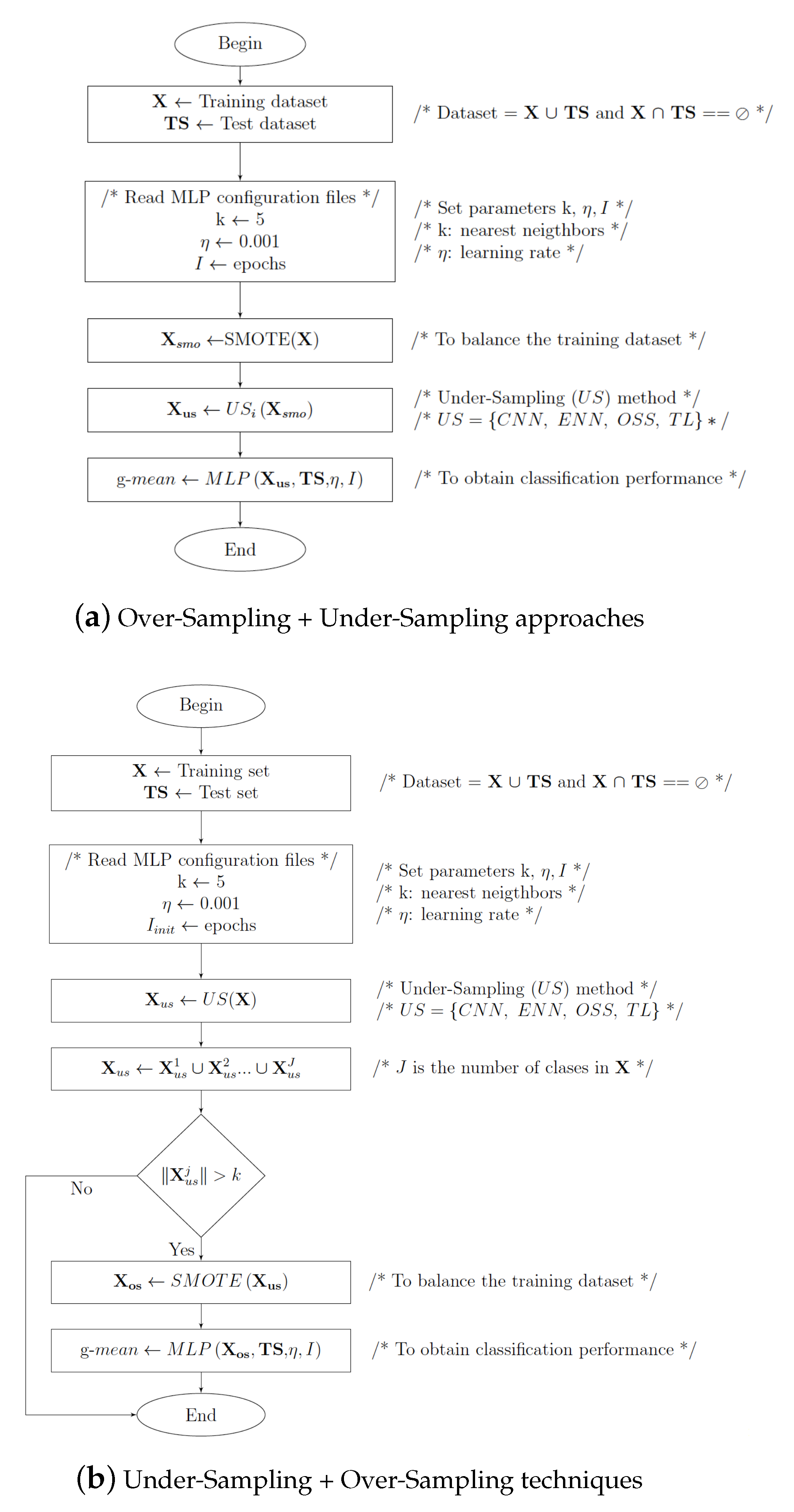
3.3. Hybrid Sampling Class Imbalance Strategies

The aim of the hybrid methods is first to deal with the class imbalance problem, and next, to clean the training dataset, in order to reduce the noise or overlap region. Hybrid methods generally employ SMOTE to compensate the class imbalance, because this method reduces the possibilities of over-training or over-fitting [1]. They use methods based in nearest neighbor rule to reduce overlap or noise in the dataset [25].

Recently, hybrid methods have increased in popularity in the machine learning community, as it can be observed in several references [23,25,66], which have studied SMOTE+TL, SMOTE+CNN and SMOTE+ENN, among others methods, to deal with class imbalance problem and to eliminate samples in the overlapping region, in order to improve the classifier performance.

SMOTE+ENN technique consists of applying the SMOTE; then, the ENN rule is applied [64]. SMOTE+TL combines SMOTE and TL [64], SMOTE+CNN performs SMOTE and then CNN [65]. Figure 1a describes the operation of these hybrid approaches, which have been widely applied to deal with the class imbalance problem [22,25,29,33,50,63,64,65,67].

The effectiveness of an additional hybrid approach is studied in this work, in which the training dataset is cleaned or reduced, and after, the number of samples by class in the training dataset is balanced. As a first stage, TL, OSS, ENN and CNN are used to clean the training dataset; in the second stage, SMOTE is applied to balance the class distribution.

SMOTE+OSS is the combination of SMOTE and OSS, in that order. TL+SMOTE first applies TL, and then SMOTE. In CNN+SMOTE, CNN is performed, and then SMOTE. Figure 1b shows the operation of these hybrid methods.

3.4. SMOTE+ENN*

Artificial Neural Networks (ANN) are computational models that have become a popular tool used in classification and regression tasks [57]. Nevertheless, it is well know that their maximum performances in supervised classification depend on the quality of the training dataset [68]. Typical methods to improve the training dataset quality are based in the nearest neighbor rule (for example: ENN, CNN, TL or OSS), which work in the feature space of the dataset. In other words, the decision region is defined in the feature space [69]. ANN sets the decision boundary in the hidden space or transformed data (see Equations (1)–(3) [55], even the deep learning ANN [70]. Thus, in this research, we consider the most appropriate scheme seeking the noise or overlap samples in the ANN hidden space (transformed data) or in the ANN output; for simplicity, we chose the last one to propose the SMOTE+ENN* approach.

SMOTE+ENN* is presented in Algorithm 1, which works as follows: first, the dataset is processed with SMOTE (Step 2); then, it is used to train the neural network (Step 5); after that, the neural network output is processed with ENN method (Step 7); i.e., the samples (of the training dataset) related to neural network output (which are considered noise) are deleted (Step 8). Finally, the neural network is trained again with the resultant dataset (Step 9). Source code of the proposed strategy is available in website (https://github.com/ccastore/SMOTE-ENN_out.git).

Algorithm 1: SMOTE+ENN*

Input: Training dataset X; Test dataset TS; // X ∩TS $==\oslash$, i.e., they are a disjunts sets.  Output: g-mean values; 1: Read MLP, SMOTE and ENN configuration files; INIT( ): 2: X${}_{smo}=$ SMOTE(X); 3: index$=\{0,1,2,3,\dots ,\parallel$X${}_{smo}\parallel \}$; 4: X${}_{idx}=({\mathbf{X}}_{smo}\mid {\mathbf{index}}^{\mathrm{T}}$); // To add index to X${}_{smo}$ 5: OUT = MLP (X${}_{idx}$, $I_{init}$); // $I_{init}$ is the number the initial epochs 6: OUT${}_{idx}=(\mathbf{OUT}\mid {\mathbf{index}}^{\mathrm{T}}$); 7: OUT${}_{enn}=$ ENN(OUT${}_{idx}$); 8: X = REMOVE(X${}_{idx}$, OUT${}_{enn}$) ; //Remove samples (from X${}_{idx}$) related to neural network output that are considered noise 9: g-$mean=$ MLP (X, TS, $I_{end}$); // To train the MLP with $I_{end}$ epochs and to test it with TS END( ) REMOVE(X${}_{idx}$, OUT${}_{enn}$): 10: /* Q and N are the number of samples and features in X${}_{idx}$, respectively.*/ 11: for$q=0$ to $q<Q$ do 12:  if $X_{idx}\left[q\right]\left[N\right]==OU{T}_{enn}\left[q\right]\left[N\right]$ then 13:   for $n=0$ to $n<(N-1)$ do 14:    // (N-1) because, the add index is deleted (Step 4). 15:    $X_{tmp}\left[q\right]\left[n\right]=X_{idx}\left[q\right]\left[n\right]$; 16:   end for 17:  end if 18: end for 19: return X${}_{tmp}$;

4. Experimental Set-Up

4.1. Database Description

The dataset of images used in this work was obtained from GIC (Grupo de Inteligencia Computacional, by the acronym in Spanish) (http://www.ehu.eus/ccwintco/index.php/Hyperspectral_Remote_Sensing_Scenes). The dataset corresponds to six hyper-spectral images with multiple bands of light ranging from the ultraviolet to the infrared spectrum; the number of bands depends on the sensors used to capture the images. In

Table 1. Summary of the main database characteristics, such as dataset name, and the numbers of classes, samples and features. Major and Minor correspond to majority and minority classes, respectively. Imbalance ratio IR = Minor/Major, and Distribution is the number of samples by class.

Data Set	Classes	Samples	Features	Major	Minor	IR	Distribution
Indian	17	21,025	220	10,776	20	538.8	0:10776; 1:46; 2:1428; 3:830; 4:237; 5:483; 6:730; 7:28; 8:478; 9:20; 10:972; 11:2455; 12::593; 13:205; 14:1265; 15:386; 16:93
Salinas	17	111,104	224	56,975	916	62.2	0:10776; 1:2009; 2:3726; 3:1976; 4:1394; 5:2678; 6:3959; 7:3579; 8:11271; 9:6203; 10:3278; 11:1068; 12:1927; 13:916; 14:1070; 15:7268; 16:1807
PaviaU	10	207,400	103	164,624	947	173.8	0:164624; 1:6631; 2:18649; 3:2099; 4:3064; 5:1345; 6:5029; 7:1330; 8::3682; 9:947
Pavia	10	783,640	102	635,488	2685	236.7	0:635488; 1:65971; 2:7598; 3:3090; 4:2685; 5:6584; 6:9248; 7:7287; 8:42826; 9:2863
Botswana	15	377,856	145	374,608	95	3943.2	0:374608; 1:270; 2:101; 3:251; 4:215; 5:269; 6:269; 7:259; 8:203; 9:314; 10:248; 11:305; 12:181; 13:268; 14:95
KSC	14	314,368	176	309,157	105	2944.4	0:309157; 1:761; 2:243; 3:256; 4:252; 5:161; 6:229; 7:105; 8:431; 9:520; 10:404; 11:419; 12:503; 13:927

, the number of bands corresponds to the number of features. Every dataset was previously tagged in order to generate a distribution of the pixels, in accordance with the class that was tagged, the number of the classes and the index of the imbalance.

The Indian and Salinas datasets were captured by the AVIRIS sensor in north-western Indiana and Salinas Valley, California, respectively; both image datasets have 17 classes that correspond to crops, grass, stone, buildings and other types. In the north of Italy, the sensor ROSES acquired the images Pavia and PaviaU with 102 and 103 spectral bands belonging to visible water, trees and shadows, among others classes. The Botswana dataset was gather in 2004 by the sensor EO-1 in the region of over the Okavango Delta, Botswana, where 15 classes were identified representing the types of swamps and woodlands. Finally, the KSC (Kennedy Space Center in Florida) has 14 classes representing the various land types. The hold-out method [68] was used to randomly split each dataset: training (X) 70% and testing (TS) 30%.

Table 1 summarizes the main characteristics and details of the benchmarking datasets, where "Major" and "Minor" correspond to number of samples of the bigger and smaller majority and minority classes, respectively; "IR" is the class imbalance ratio between both classes (Minor/Major); and "Distribution" shows the number of samples in each class.

4.2. Parameter Specification for the Algorithms Used in the Experimentation

The sampling methods used in this work can be found as a part of the library $imblearn$ (https://pypi.org/project/imblearn/). It includes the over-sampling techniques SMOTE, ROS and ADASYN, and the under-sampling methods RUS, TL, ENN and OSS. All of them were implemented in Python programming language and could be performed in multi-class datasets. These methods were applied with default set-up ($k=5$) and the random state or seed was set to 42. In the case of the hybrid methods, the same library was used following the steps depicted in Figure 1, where over-sampling or under-sampling methods were performed in the original dataset, and the new dataset was processed with the other sampling method; afterwards, it was used for training of the neural network.

Multiple configurations of hidden layers and neurons (or nodes) for each neural network were employed. Both hidden layers and nodes were obtained for a trial and error strategy for every dataset.

Table 2. Neural networks’ parameters and specification used in the experimentation stage. The first column shows the dataset name. In the following columns: the number of hidden layers and its parameter (number of hidden neurons and activation function used in the respective layer). Layer output indicates the number of output neurons and the activation function to these nodes. Epoch is the number of epochs employed in the training. Size of Batch is the portion of samples used for the deep neural networks in each epoch.

Name	Layer Int	Layer 1	Layer 2	Layer 3	Layer 4	Layer 5	Layer 6	Layer Output	Epoch	Size of Batch
Salinas	220/Relu	60/Relu	60/Relu	60/Relu	60/Relu	60/Relu	60/Relu	17/SoftMax	500	1000
Indian	224/Relu	60/Relu	60/Relu	60/Relu	60/Relu	–	–	17/SoftMax	500	100
PaviaU	103/Relu	40/Relu	40/Relu	40/Relu	40/Relu	40/Relu	–	10/SoftMax	500	1000
Pavia	102/Relu	40/Relu	40/Relu	40/Relu	40/Relu	40/Relu	40/Relu	10/SoftMax	250	1000
Botswana	145/Relu	30/Relu	30/Relu	30/Relu	30/Relu	30/Relu	30/Relu	15/SoftMax	250	1000
KSC	176/Relu	60/Relu	60/Relu	60/Relu	60/Relu	60/Relu	60/Relu	14/SoftMax	250	1000

shows the neural networks’ free parameters and the specifications employed in the experimentation stage. The learning rate ($\eta$) was set to $0.001$ and the stopping criterion was established at 500; 250 epochs were used for SMOTE+ENN* (for the proposed method, Algorithm 1) if the MSE value was lower than $0.001$. The training of the neural network was performed by means of the Adam method; the latter is a computationally efficient and simple algorithm for optimization of stochastic objective functions by the gradient descent principle [59]. The training process was performed ten times in the experimental stage and the results correspond to the averages of those runs.

4.3. Classifier Performance and Tests of Statistical Significance

The geometric mean (g-mean) is the most widely used method to evaluate the performance of classifiers and it is a well recognized tool for the evaluation in the class imbalance context; it is defined as follows [17]:

$$g-mean=\sqrt[J]{\prod _{j=1}^{J}ac{c}_j}$$

(5)

where $acc$ is the accuracy by class, and J is the number of classes in the dataset.

In order to strengthen the results analysis, a non-parametric statistical test was additionally achieved. Friedman test is a non-parametric method in which the first step is to rank the algorithms for each dataset separately; the best performing algorithm should have rank 1, the second best rank 2, etc. In the case of ties, average ranks are computed. Friedman test uses the average rankings to calculate Friedman statistic, which can be computed as follows:

$${\chi }_F^2=\frac{12N}{K(K+1)}(\sum _j{R}_j^2-\frac{K{(K+1)}^2}{4})$$

(6)

K denotes the number of methods, N the number of data sets and $R_j$ the average rank of method j on all datasets.

On the other hand, Iman and Davenport [71] demonstrated that ${\chi }_F^2$ has a conservative behavior. They proposed Equation (7) according to F–distribution with $K-1$ and $(K-1)(N-1)$ Degrees of Freedom, as a better statistic:

$$F_F=\frac{(N-1){\chi }_F^2}{N(K-1)-{\chi }_F^2}$$

(7)

Friedman and Iman–Davenport tests were used in this investigation, by using the level of confidence $\gamma =0.05$ and KEEL software [72].

5. Experimental Results and Discussion

Table 3. DL-MLP performance using the g-mean (Equation (5)) as measure. Values presented correspond to averages of ten different initializations of the neural network weights.

	Method	Indian	Salinas	PaviaU	Pavia	Botswana	KSC	Average Rank
	Original	0.8848	0.0000	0.5369	0.0000	0.0000	0.0000	11.1
Under-sampling	RUS	0.8834	0.4280	0.7369	0.8460	0.4594	0.5640	9.5
	TL	0.8891	0.0000	0.5272	0.0000	0.0000	0.0000	11.1
	ENN	0.8728	0.0000	0.3809	0.0000	0.0000	0.0000	11.8
	OSS+SMOTE	N/A	N/A	N/A	N/A	N/A	N/A	N/A
Over-sampling	ROS	0.9627	0.8202	0.8723	0.8984	0.7243	0.6752	3.7
	SMOTE	0.9603	0.8140	0.8704	0.8892	0.7256	0.7284	4.4
	ADASYN	0.9603	0.8037	0.8633	0.8892	0.7462	0.6974	5.1
Hybrid	SMOTE+ENN*	0.8201	0.9542	0.8797	0.9074	0.8139	0.7863	2.5
	SMOTE+ENN	0.9610	0.8138	0.8670	0.8879	0.7346	0.7076	5.0
	SMOTE+TL	0.9610	0.8068	0.8609	0.8812	0.7410	0.7177	5.0
	SMOTE+OSS	0.0000	0.0000	0.8684	0.8888	0.7372	0.7410	6.8
	TL+SMOTE	0.9604	0.7706	0.8522	0.8747	0.6554	0.6079	7.5
	SMOTE+CNN	0.0000	0.0000	0.8417	0.0000	0.8657	0.8200	7.7
	ENN+SMOTE	0.9274	N/A	0.6331	0.4996	N/A	N/A	N/A
	CNN+SMOTE	N/A	N/A	N/A	N/A	N/A	N/A	N/A
	OSS+SMOTE	N/A	N/A	N/A	N/A	N/A	N/A	N/A

exhibits the g-mean values for each method and dataset. Friedman ranks were added in order to simplify the understanding of the results (see Section 4.3). Table 3 confirms previous machine learning works, in the sense that other problems, such as class overlapping, the small disjuncts, the lack of density or the noisy data, among others, increase the effect of class imbalance on the classifier performance. For example, see the Salinas dataset, which is a high imbalanced dataset and its g-mean value (without a preprocessing method) is relatively high (0.8848); i.e, it is affected by the class imbalance, but this problem does not induce a poor classification performance (as it occurs in other datasets).

These results highlighted the need to study a heuristic methods that allow one improve the quality of the training dataset, such as ENN, or strategies such as TL or CNN (see Section 3), in order to reduce the negative effect of the class imbalance on the classifier performance.

For the rest of datasets, the classifier performance is clearly impacted by the class imbalance problem, as it can be observed in Table 3. When the classes distribution was balanced, a substantial performance improvement was reached (see ROS and SMOTE results).

In accordance with Friedman ranks, it can be noted that ROS presents better results than SMOTE. In machine learning scenarios, SMOTE traditionally overcomes ROS’s performance [24], but in the big data and deep learning context, results (of this work) show that this expectation was not sufficiently fulfilled. This behavior has been observed in other works related to big data and deep learning [1,48]. However, the performances of both ROS and SMOTE were practically equivalent. Even for the KSC dataset, SMOTE g-mean outperforms ROS, although there does exist a clear trend to obtain better results with ROS than with SMOTE.

RUS overcomes the classification performance of MLP trained with the original dataset; notwithstanding, it only improves the g-mean results of TL and ENN. I.e., RUS is an effective technique to deal with the class imbalance problem, but it is not the best strategy. RUS eliminates a considerable amount of samples and keeps acceptable values of g-mean in Salinas, Pavia and PaviaU. These results exhibit that only a few samples are necessary to obtain a good classifier performance; thus, this information gives relevance to the study of heuristic sampling data.

On the other hand, Table 3 shows that in the most datasets, the strategies ENN and TL present the worst results. In Indian, Pavia, Botswana and KCS datasets it is not enough only to improve the quality of the data to increase the classification performance, but when they are added to any over-sampling method, the classification performance is improved. However, Table 3 does not show that g-means from SMOTE+ENN and SMOTE+TL overcome the g-mean of SMOTE. Analyzing the SMOTE+CNN and SMOTE+OSS methods, a similar classification performance behavior was observed.

CNN, ENN, TL and OSS are effective methods with which to improve the training dataset quality in nearest neighbor rule context; in neural networks, only ENN combined with SMOTE archives positive results, but it does not generate better results than SMOTE. In addition, CNN+SMOTE, OSS+SMOTE and ENN+SMOTE show values N/A (i.e., does not apply), which make reference to situations where these editing methods eliminate too many samples from a particular class. SMOTE is not applicable in such cases because it needs a least six samples by class; some classes of those methods only keep less than six samples, and it is proposed to not consider these values for this reason.

CNN is a method to keep a consistent subset from the training data, in the way that all samples in a consistent subset are successfully classified by nearest neighbor rule [28]. Therefore, methods that are successful by nearest neighbor rules are not necessarily effective in a neural network context.

ENN, TL, OSS and CNN are methods based in nearest neighbor rule [73], whose decision boundaries are defined locally in the feature space. However, the decision boundary in MLP neural networks is defined in the hidden space, not in the feature space [8]. Thus, it is assumed that to apply these editing methods in the data features space, i.e., in the training data, is not the best option because these methods help to determine the decision boundary to nearest neighbor rule, not for neural network classifier. For this reason, in order to remove samples that make it difficult to set the neural network decision boundary, the ENN is applied in the neural network output in this work.

The proposed method SMOTE+ENN* (Algorithm 1) consists of training the neural network during $I_{init}=250$ epochs, and next applying ENN in the neural network output. In other words, it removes the samples suspected of being outliers or noise from the training data, which correspond to those identified in the neural network output space for the ENN. Following that, the neural network was trained again ($I_{end}=250$) with the resultant dataset. Results presented in Table 3 show that there was a trend to obtain the best results when the neural network output was edited. SMOTE+ENN* presents the best average rank (2.5); i.e., it is better than the ranks for ROS (3.7) and SMOTE (4.4). These results evidence the appropriateness of sampling the neural network output, instead of preprocessing the input feature space.

Finally, the Friedman and Iman–Davenport non-parametrical statistical tests were applied to five best sampling methods (SMOTE+ENN*, ROS, SMOTE, SMOTE+ENN and SMOTE+TL) in order to know if a significant difference exists in these methods.

Results report that considering the reduction in performance distributed according to chi-square with four Degrees of Freedom, the Friedman statistic was set to 5.73 and p-value computed by the Friedman test was 0.219. Considering the performance reduction according to F-distribution with 13 and 143 Degrees of Freedom, the Iman and Davenport statistic was 1.57, and the p-value computed by the Iman–Davenport test was 0.221. Thus, the null hypothesis is accepted given that Friedman and Iman–Davenport tests indicate that there are not significant differences in the results. In others words, the performances of these five methods are statistically equivalent. Notwithstanding, in the results exist evidence of the importance of applying the sampling methods in the neural network output.

6. Conclusions and Future Work

In this work, the potential of the heuristic sampling strategies to deal with the multi-class imbalance problem on DL-MLP neural network in big data scenarios was studied. Big data, multi-class imbalanced datasets obtained from hyperspectral remote sensing images were used for experimentation. Results presented in this work exhibit that ROS and SMOTE are very competitive strategies to deal with this problem, but ROS shows a better performance than SMOTE.

Hybrid methods such as SMOTE+TL, SMOTE+ENN, SMOTE+OSS and SMOTE+CNN, although presenting evidence of being effective techniques for facing the class imbalance problem, do not improve the SMOTE’s performance. Cleaning and sampling reduction strategies (TL, ENN, OSS and CNN) do not show results with respect to a DL-MLP neural network on big data scenarios.

RUS gives evidence of that with a few samples, favorable results can be obtained, but they are not better (or competitive) than the results of ROS and SMOTE. However, RUS results strengthen the hypothesis that with a small subset, the DL-MLP neural network can be successfully trained.

In this study it was found that cleaning strategies should be applied on ANN output instead of input feature space, in order to obtain the best classification results. Thus, SMOTE+ENN* is proposed, which consists of training the neural network, applying ENN on the neural network’s output and removing those samples (from the training dataset) related to neural network outputs suspicious to be outliers or noise; i.e., those outputs identified by ENN. Results presented in this work evidence a trend to obtain better results when a neural network’s output is edited than when input feature space is preprocessed.

Typically, most of the research reported in literature has been focused on the two-class imbalance problem by using classical classifiers. Thus, the study of the relevance and capabilities of heuristic sampling methods to deal with the big data multi-class imbalance problem in deep learning context is especially interesting.

Future work should be addressed toward deep learning, in the study of reduction and cleaning strategies to improve the DL-MLP neural network’s performance in big data scenarios.

References

1. Basgall, M.J.; Hasperué, W.; Naiouf, M.; Fernández, A.; Herrera, F. An Analysis of Local and Global Solutions to Address Big Data Imbalanced Classification: A Case Study with SMOTE Preprocessing. In Cloud Computing and Big Data; Naiouf, M., Chichizola, F., Rucci, E., Eds.; Springer International Publishing: Cham, Switzerland, 2019; pp. 75–85. [Google Scholar]
2. Fernández, A.; del Río, S.; Chawla, N.V.; Herrera, F. An insight into imbalanced Big Data classification: Outcomes and challenges. Complex Intell. Syst. 2017, 3, 105–120. [Google Scholar] [CrossRef] [Green Version]
3. Elshawi, R.; Sakr, S.; Talia, D.; Trunfio, P. Big Data Systems Meet Machine Learning Challenges: Towards Big Data Science as a Service. Big Data Res. 2018, 14, 1–11. [Google Scholar] [CrossRef] [Green Version]
4. Oussous, A.; Benjelloun, F.Z.; Lahcen, A.A.; Belfkih, S. Big Data technologies: A survey. J. King Saud Univ. Comput. Inf. Sci. 2018, 30, 431–448. [Google Scholar] [CrossRef]
5. Guo, Y.; Liu, Y.; Oerlemans, A.; Lao, S.; Wu, S.; Lew, M.S. Deep learning for visual understanding: A review. Neurocomputing 2016, 187, 27–48. [Google Scholar] [CrossRef]
6. Reyes-Nava, A.; Sánchez, J.; Alejo, R.; Flores-Fuentes, A.; Rendón-Lara, E. Performance Analysis of Deep Neural Networks for Classification of Gene-Expression microarrays. In Proceedings of the Pattern Recognition—10th Mexican Conference, MCPR 2018, Puebla, Mexico, 27–30 June 2018; Volume 10880, pp. 105–115. [Google Scholar] [CrossRef]
7. LeCun, Y.; Bengio, Y.; Hinton, G. Deep Learning. Nature 2015, 521, 436–444. [Google Scholar] [CrossRef] [PubMed]
8. Goodfellow, I.; Bengio, Y.; Courville, A. Deep Learning; MIT Press: Cambridge, MA, USA, 2016. [Google Scholar]
9. Zaharia, M.; Xin, R.S.; Wendell, P.; Das, T.; Armbrust, M.; Dave, A.; Meng, X.; Rosen, J.; Venkataraman, S.; Franklin, M.J.; et al. Apache Spark: A Unified Engine for Big Data Processing. Commun. ACM 2016, 59, 56–65. [Google Scholar] [CrossRef]
10. Abadi, M.; Barham, P.; Chen, J.; Chen, Z.; Davis, A.; Dean, J.; Devin, M.; Ghemawat, S.; Irving, G.; Isard, M.; et al. TensorFlow: A System for Large-scale Machine Learning. In Proceedings of the 12th USENIX Conference on Operating Systems Design and Implementation, OSDI’16, USENIX Association, Savannah, GA, USA, 2–4 November 2016; pp. 265–283. [Google Scholar]
11. Lin, T.; Goyal, P.; Girshick, R.; He, K.; Dollár, P. Focal Loss for Dense Object Detection. In Proceedings of the 2017 IEEE International Conference on Computer Vision (ICCV), Venice, Italy, 22–29 October 2017; pp. 2999–3007. [Google Scholar] [CrossRef] [Green Version]
12. Buda, M.; Maki, A.; Mazurowski, M.A. A systematic study of the class imbalance problem in convolutional neural networks. Neural Netw. 2018, 106, 249–259. [Google Scholar] [CrossRef] [PubMed] [Green Version]
13. Khan, S.H.; Hayat, M.; Bennamoun, M.; Sohel, F.A.; Togneri, R. Cost-Sensitive Learning of Deep Feature Representations From Imbalanced Data. IEEE Trans. Neural Netw. Learn. Syst. 2018, 29, 3573–3587. [Google Scholar] [PubMed] [Green Version]
14. Yang, K.; Yu, Z.; Wen, X.; Cao, W.; Chen, C.L.P.; Wong, H.; You, J. Hybrid Classifier Ensemble for Imbalanced Data. IEEE Trans. Neural Netw. Learn. Syst. 2019, 1–14. [Google Scholar] [CrossRef] [PubMed]
15. Wong, M.L.; Seng, K.; Wong, P.K. Cost-sensitive ensemble of stacked denoising autoencoders for class imbalance problems in business domain. Expert Syst. Appl. 2020, 141, 112918. [Google Scholar] [CrossRef]
16. Błaszczyński, J.; Stefanowski, J. Local Data Characteristics in Learning Classifiers from Imbalanced Data. In Advances in Data Analysis with Computational Intelligence Methods: Dedicated to Professor Jacek Żurada; Springer International Publishing: Cham, Switzerland, 2018; pp. 51–85. [Google Scholar] [CrossRef]
17. Leevy, J.L.; Khoshgoftaar, T.M.; Bauder, R.A.; Seliya, N. A survey on addressing high-class imbalance in big data. J. Big Data 2018, 5, 42. [Google Scholar] [CrossRef]
18. González-Barcenas, V.M.; Rendón, E.; Alejo, R.; Granda-Gutiérrez, E.E.; Valdovinos, R.M. Addressing the Big Data Multi-class Imbalance Problem with Oversampling and Deep Learning Neural Networks. In Pattern Recognition and Image Analysis; Morales, A., Fierrez, J., Sánchez, J.S., Ribeiro, B., Eds.; Springer International Publishing: Cham, Switzerland, 2019; pp. 216–224. [Google Scholar]
19. Kubat, M.; Matwin, S. Addressing the curse of imbalanced training sets: One-sided selection. In Proceedings of the 14th International Conference on Machine Learning, Nashville, TN, USA, 8–12 July 1997; Morgan Kaufmann: Burlington, MA, USA, 1997; pp. 179–186. [Google Scholar]
20. Yıldırım, P. Pattern Classification with Imbalanced and Multiclass Data for the Prediction of Albendazole Adverse Event Outcomes. Procedia Comput. Sci. 2016, 83, 1013–1018. [Google Scholar] [CrossRef] [Green Version]
21. Fernández, A.; García, S.; Galar, M.; Prati, R.C.; Krawczyk, B.; Herrera, F. Learning from Imbalanced Data Sets; Springer International Publishing: Cham, Switzerland, 2018. [Google Scholar] [CrossRef]
22. Prati, R.C.; Batista, G.E.; Monard, M.C. Data mining with imbalanced class distributions: Concepts and methods. In Proceedings of the 4th Indian International Conference on Artificial Intelligence, IICAI 2009, Tumkur, India, 16–18 December 2009; pp. 359–376. [Google Scholar]
23. Vuttipittayamongkol, P.; Elyan, E. Neighbourhood-based undersampling approach for handling imbalanced and overlapped data. Inf. Sci. 2020, 509, 47–70. [Google Scholar] [CrossRef]
24. Fernandez, A.; Garcia, S.; Herrera, F.; Chawla, N.V. SMOTE for Learning from Imbalanced Data: Progress and Challenges, Marking the 15-year Anniversary. J. Artif. Intell. Res. 2018, 61, 863–905. [Google Scholar] [CrossRef]
25. García, V.; Sánchez, J.; Marqués, A.; Florencia, R.; Rivera, G. Understanding the apparent superiority of over-sampling through an analysis of local information for class-imbalanced data. Expert Syst. Appl. 2019, 113026, in press. [Google Scholar] [CrossRef]
26. Tomek, I. Two Modifications of CNN. IEEE Trans. Syst. Man Cybern. 1976, 7, 679–772. [Google Scholar]
27. Wilson, D. Asymptotic properties of nearest neighbor rules using edited data. IEEE Trans. Syst. Man Cybern. 1972, 2, 408–420. [Google Scholar] [CrossRef] [Green Version]
28. Hart, P. The Condensed Nearest Neighbour Rule. IEEE Trans. Inf. Theory 1968, 14, 515–516. [Google Scholar] [CrossRef]
29. He, H.; Garcia, E. Learning from Imbalanced Data. IEEE Trans. Knowl. Data Eng. 2009, 21, 1263–1284. [Google Scholar] [CrossRef]
30. López, V.; Fernández, A.; García, S.; Palade, V.; Herrera, F. An insight into classification with imbalanced data: Empirical results and current trends on using data intrinsic characteristics. Inf. Sci. 2013, 250, 113–141. [Google Scholar] [CrossRef]
31. Nanni, L.; Fantozzi, C.; Lazzarini, N. Coupling Different Methods for Overcoming the Class Imbalance Problem. Neurocomputing 2015, 158, 48–61. [Google Scholar] [CrossRef] [Green Version]
32. Abdi, L.; Hashemi, S. To Combat Multi-class Imbalanced Problems by Means of Over-sampling Techniques. IEEE Trans. Knowl. Data Eng. 2016, 28, 1041–4347. [Google Scholar] [CrossRef]
33. Devi, D.; kr. Biswas, S.; Purkayastha, B. Redundancy-driven modified Tomek-link based undersampling: A solution to class imbalance. Pattern Recognit. Lett. 2017, 93, 3–12. [Google Scholar] [CrossRef]
34. Zhou, Z.H.; Liu, X.Y. Training cost-sensitive neural networks with methods addressing the class imbalance problem. IEEE Trans. Knowl. Data Eng. 2006, 18, 63–77. [Google Scholar] [CrossRef]
35. Shon, H.S.; Batbaatar, E.; Kim, K.O.; Cha, E.J.; Kim, K.A. Classification of Kidney Cancer Data Using Cost-Sensitive Hybrid Deep Learning Approach. Symmetry 2020, 12, 154. [Google Scholar] [CrossRef] [Green Version]
36. Chris, D.; Robert C., H. C4.5, Class Imbalance, and Cost Sensitivity: Why Under-sampling beats Over-sampling. In Workshop on Learning from Imbalanced Datasets II; Citeseer: Washington, DC, USA, 2003; pp. 1–8. [Google Scholar]
37. Kukar, M.; Kononenko, I. Cost-Sensitive Learning with Neural Networks. In Proceedings of the 13th European Conference on Artificial Intelligence (ECAI-98), Brighton, UK, 23–28 August 1998; pp. 445–449. [Google Scholar]
38. Wang, S.; Yao, X. Multiclass Imbalance Problems: Analysis and Potential Solutions. IEEE Trans. Syst. Man Cybern. Part B 2012, 42, 1119–1130. [Google Scholar] [CrossRef]
39. Galar, M.; Fernández, A.; Tartas, E.B.; Sola, H.B.; Herrera, F. A Review on Ensembles for the Class Imbalance Problem: Bagging-, Boosting-, and Hybrid-Based Approaches. IEEE Trans. Syst. Man Cybern. Part C 2012, 42, 463–484. [Google Scholar] [CrossRef]
40. He, H.; Ma, Y. Imbalanced Learning: Foundations, Algorithms, and Applications, 1st ed.; Wiley-IEEE Press: Hoboken, NJ, USA, 2013. [Google Scholar]
41. Parvin, H.; Minaei-Bidgoli, B.; Alinejad-Rokny, H. A New Imbalanced Learning and Dictions Tree Method for Breast Cancer Diagnosis. J. Bionanosci. 2013, 7, 673–678. [Google Scholar] [CrossRef]
42. Sun, T.; Jiao, L.; Feng, J.; Liu, F.; Zhang, X. Imbalanced Hyperspectral Image Classification Based on Maximum Margin. IEEE Geosci. Remote Sens. Lett. 2015, 12, 522–526. [Google Scholar] [CrossRef]
43. Pandey, S.K.; Mishra, R.B.; Tripathi, A.K. BPDET: An effective software bug prediction model using deep representation and ensemble learning techniques. Expert Syst. Appl. 2020, 144, 113085. [Google Scholar] [CrossRef]
44. García-Gil, D.; Holmberg, J.; García, S.; Xiong, N.; Herrera, F. Smart Data based Ensemble for Imbalanced Big Data Classification. arXiv 2020, arXiv:2001.05759. [Google Scholar]
45. Li, Q.; Song, Y.; Zhang, J.; Sheng, V.S. Multiclass imbalanced learning with one-versus-one decomposition and spectral clustering. Expert Syst. Appl. 2020, 147, 113152. [Google Scholar] [CrossRef]
46. Tao, X.; Li, Q.; Guo, W.; Ren, C.; He, Q.; Liu, R.; Zou, J. Adaptive weighted over-sampling for imbalanced datasets based on density peaks clustering with heuristic filtering. Inf. Sci. 2020, 519, 43–73. [Google Scholar] [CrossRef]
47. Andresini, G.; Appice, A.; Malerba, D. Dealing with Class Imbalance in Android Malware Detection by Cascading Clustering and Classification. In Complex Pattern Mining: New Challenges, Methods and Applications; Appice, A., Ceci, M., Loglisci, C., Manco, G., Masciari, E., Ras, Z.W., Eds.; Springer International Publishing: Cham, Switzerland, 2020; pp. 173–187. [Google Scholar] [CrossRef]
48. Reyes-Nava, A.; Cruz-Reyes, H.; Alejo, R.; Rendón-Lara, E.; Flores-Fuentes, A.A.; Granda-Gutiérrez, E.E. Using Deep Learning to Classify Class Imbalanced Gene-Expression Microarrays Datasets. In Progress in Pattern Recognition, Image Analysis, Computer Vision, and Applications; Vera-Rodriguez, R., Fierrez, J., Morales, A., Eds.; Springer International Publishing: Cham, Switzerland, 2019; pp. 46–54. [Google Scholar]
49. Amin, A.; Anwar, S.; Adnan, A.; Nawaz, M.; Howard, N.; Qadir, J.; Hawalah, A.; Hussain, A. Comparing Oversampling Techniques to Handle the Class Imbalance Problem: A Customer Churn Prediction Case Study. IEEE Access 2016, 4, 7940–7957. [Google Scholar] [CrossRef]
50. Zhang, Y.; Chen, X.; Guo, D.; Song, M.; Teng, Y.; Wang, X. PCCN: Parallel Cross Convolutional Neural Network for Abnormal Network Traffic Flows Detection in Multi-Class Imbalanced Network Traffic Flows. IEEE Access 2019, 7, 119904–119916. [Google Scholar] [CrossRef]
51. Bhowmick, K.; Shah, U.B.; Shah, M.Y.; Parekh, P.A.; Narvekar, M. HECMI: Hybrid Ensemble Technique for Classification of Multiclass Imbalanced Data. In Information Systems Design and Intelligent Applications; Satapathy, S.C., Bhateja, V., Somanah, R., Yang, X.S., Senkerik, R., Eds.; Springer: Singapore, 2019; pp. 109–118. [Google Scholar]
52. Shekar, B.H.; Dagnew, G. Classification of Multi-class Microarray Cancer Data Using Ensemble Learning Method. In Data Analytics and Learning; Nagabhushan, P., Guru, D.S., Shekar, B.H., Kumar, Y.H.S., Eds.; Springer: Singapore, 2019; pp. 279–292. [Google Scholar]
53. Cao, J.; Lv, G.; Chang, C.; Li, H. A Feature Selection Based Serial SVM Ensemble Classifier. IEEE Access 2019, 7, 144516–144523. [Google Scholar] [CrossRef]
54. Li, D.; Huang, F.; Yan, L.; Cao, Z.; Chen, J.; Ye, Z. Landslide Susceptibility Prediction Using Particle-Swarm-Optimized Multilayer Perceptron: Comparisons with Multilayer-Perceptron-Only, BP Neural Network, and Information Value Models. Appl. Sci. 2019, 9, 3664. [Google Scholar] [CrossRef] [Green Version]
55. Haykin, S. Neural Networks. A Comprehensive Foundation, 2nd ed.; Pretince Hall: Upper Saddle River, NJ, USA, 1999. [Google Scholar]
56. Lecun, Y.; Bottou, L.; Orr, G.B.; Müller, K.R. Efficient BackProp. In Neural Networks—Tricks of the Trade; Orr, G., Müller, K., Eds.; Lecture Notes in Computer Science; Springer: Berlin/Heidelberg, Germany, 1998; Volume 1524, pp. 5–50. [Google Scholar]
57. Pacheco-Sánchez, J.; Alejo, R.; Cruz-Reyes, H.; Álvarez Ramírez, F. Neural networks to fit potential energy curves from asphaltene-asphaltene interaction data. Fuel 2019, 236, 1117–1127. [Google Scholar] [CrossRef]
58. Ruder, S. An overview of gradient descent optimization algorithms. arXiv 2016, arXiv:1609.04747. [Google Scholar]
59. Kingma, D.P.; Ba, J. Adam: A method for stochastic optimization. arXiv 2014, arXiv:1412.6980. [Google Scholar]
60. Japkowicz, N.; Stephen, S. The class imbalance problem: A systematic study. Intell. Data Anal. 2002, 6, 429–449. [Google Scholar] [CrossRef]
61. Chawla, N.V.; Bowyer, K.W.; Hall, L.O.; Kegelmeyer, W.P. SMOTE: Synthetic Minority Over-sampling Technique. J. Artif. Intell. Res. 2002, 16, 321–357. [Google Scholar] [CrossRef]
62. He, H.; Bai, Y.; Garcia, E.A.; Li, S. ADASYN: Adaptive synthetic sampling approach for imbalanced learning. In Proceedings of the 2008 IEEE International Joint Conference on Neural Networks (IEEE World Congress on Computational Intelligence), Hong Kong, China, 1–8 June 2008; pp. 1322–1328. [Google Scholar] [CrossRef] [Green Version]
63. Alejo, R.; Monroy-de Jesús, J.; Pacheco-Sánchez, J.; López-González, E.; Antonio-Velázquez, J. A Selective Dynamic Sampling Back-Propagation Approach for Handling the Two-Class Imbalance Problem. Appl. Sci. 2016, 6, 200. [Google Scholar] [CrossRef] [Green Version]
64. Batista, G.E.; Prati, R.C.; Monard, M.C. A study of the behavior of several methods for balancing machine learning training data. SIGKDD Explor. Newsl. 2004, 6, 20–29. [Google Scholar] [CrossRef]
65. Millán-Giraldo, M.; García, V.; Sánchez, J.S. Instance Selection Methods and Resampling Techniques for Dissimilarity Representation with Imbalanced Data Sets. In Pattern Recognition—Applications and Methods; Latorre Carmona, P., Sánchez, J.S., Fred, A.L., Eds.; Springer: Berlin/Heidelberg, Germany, 2013; pp. 149–160. [Google Scholar] [CrossRef]
66. Mar, N.M.; Thidar, L.K. KNN–Based Overlapping Samples Filter Approach for Classification of Imbalanced Data. In Software Engineering Research, Management and Applications; Springer International Publishing: Cham, Switzerland, 2020; pp. 55–73. [Google Scholar] [CrossRef]
67. Marqués, A.; García, V.; Sánchez, J. On the suitability of resampling techniques for the class imbalance problem in credit scoring. J. Oper. Res. Soc. 2013, 64, 1060–1070. [Google Scholar] [CrossRef] [Green Version]
68. Duda, R.; Hart, P.; Stork, D. Pattern Classification, 2nd ed.; Wiley: New York, NY, USA, 2001. [Google Scholar]
69. Cover, T.; Hart, P. Nearest Neighbor Pattern Classification. IEEE Trans. Inf. Theory 2006, 13, 21–27. [Google Scholar] [CrossRef]
70. Li, Y.; Ding, L.; Gao, X. On the Decision Boundary of Deep Neural Networks. arXiv 2018, arXiv:1808.05385. [Google Scholar]
71. Iman, R.L.; Davenport, J.M. Approximations of the critical region of the friedman statistic. Commun. Stat. Theory Methods 1980, 9, 571–595. [Google Scholar] [CrossRef]
72. Triguero, I.; Gonzalez, S.; Moyano, J.; Garcia, S.; Alcala-Fdez, J.; Luengo, J.; Fernandez, A.; del Jesus, M.; Sanchez, L.; Herrera, F. KEEL 3.0: An Open Source Software for Multi-Stage Analysis in Data Mining. Int. J. Comput. Intell. Syst. 2017, 10, 1238–1249. [Google Scholar] [CrossRef] [Green Version]
73. Olvera-López, J.A.; Carrasco-Ochoa, J.A.; Martínez-Trinidad, J.F.; Kittler, J. A Review of Instance Selection Methods. Artif. Intell. Rev. 2010, 34, 133–143. [Google Scholar] [CrossRef]
Figure 1. Flowchart of hybrid sampling methods.
Applsci 10 01276 g001