Article

Approach to Risk Performance Reasoning with Hidden Markov Model for Bauxite Shipping Process Safety by Handy Carriers

1
Merchant Marine College, Shanghai Maritime University, Shanghai 201306, China
2
Australia Maritime College, University of Tasmania, Launceston 7248, Australia
3
Faculty of Maritime and Transportation, Ningbo University, Zhejiang 315211, China
*
Authors to whom correspondence should be addressed.
Appl. Sci. 2020, 10(4), 1269; https://doi.org/10.3390/app10041269
Submission received: 31 December 2019 / Revised: 9 February 2020 / Accepted: 11 February 2020 / Published: 13 February 2020
(This article belongs to the Special Issue Systems Engineering: Availability and Reliability)

Abstract

:
An approach based on the hidden Markov model (HMM) is proposed for risk performance reasoning (RPR) for the bauxite shipping process by Handy carriers. The unobservable (hidden) state process in the approach aims to model the underlying risk performance, while the observation process was formed from the time series of risk factors. Within the framework, the log-likelihood probability was used as the measure of similarity between historical and current data of risk reasoning factors. Based on scalar quantization regulation and risk performance quantization regulation, the RPR approach with different step sizes was conducted on the operational case, the performance of which was evaluated in terms of effectiveness and accuracy. The reasoning performance of the HMM was tested during the validation period using three simulated scenarios and one accident scenario. The results showed significant improvement in the reasoning capacity, and satisfactory performance for numerical risk reasoning and categorical performance reasoning. The proposed model is able to provide a reference for risk performance monitoring and threat pre-warning during the bauxite shipping process.

1. Introduction

Bauxite is abundant, totaling 30 billion tons globally in 2018, according to the data from the United States Geological Survey (USGS). The natural distribution of bauxite is extremely uneven, mainly concentrated in Africa, Oceania, South America, and Southeast Asia. China’s demand for imported bauxite increased sharply from about 2.3 million tons in 2007 to 82.62 million tons in 2018 [1]. Panamax and Handy carriers transport 90% of the bauxite via shipping [2]. Here, Handy carrier is the collective term that refers to Handysize and Handymax bulk carriers. Handy carriers play an important role in bauxite shipping, accounting for 48% of the total industry. Meanwhile, 74% of deaths in the industry were linked to accidents involving Handy bulk carriers [3,4,5,6]. The liquefaction of bauxite during transportation is an important cause of ship accidents, directly responsible for more than 80 casualties of seafarers [7].
The basic reason for liquefaction is that the moisture content of bauxite exceeds the transportable moisture limit (TML). Influenced by the effect of the ship’s stability and its cargo properties in a complex shipping process, bauxite with a high moisture content carried by Handy carriers tends to liquefy, which threatens the stability and safety of the ship. The bauxite performance, dynamic ship stability, and maritime environment have important effects on the risk level of the carrier during the transportation process. Risk identification and monitoring can improve the capacity for risk prevention on bauxite carriers. The study of risk reasoning of the transportation process based on cargo information and uncertain weather and sea conditions may allow more time for an emergency response, thus reducing the risk of loss or damage. A hidden Markov model (HMM)-based approach is introduced here to reveal the factor and time correlations of the observation index and hidden risk, thereby achieving risk reasoning for the bauxite transportation process.
The organization of this paper is as follows: recent studies related to bauxite liquefaction and its risk reasoning are reviewed in Section 2. The research theory and the model for reasoning are presented in Section 3. The model is applied to specific cases in Section 4, where the results are analyzed for effectiveness and accuracy. Section 5 presents the analysis and discussion of this study, encompassing scenario planning. Conclusions are drawn in Section 6.

2. Literature Review

2.1. System of Maritime Transportation

Maritime transportation is a complex process, which involves many factors such as human, ship, environment, management, and cargo. In order to carry out risk reasoning for the transportation process, it is necessary to determine any accident mechanisms related to cargo. Cargo has a complex correlation with the other subsystems in the operation safety of a ship. For example, Li [8] studied the safety evolution of seaborne dangerous chemicals under various uncertain conditions. The aforementioned research paved the way for a new mode of operation safety research for specific cargo ships. Unlike dangerous chemicals, cargoes that may liquefy are not inherently dangerous. Nevertheless, danger can occur when cargoes start moving on the carrier. Ma [9] studied the shipping risk of ore concentrate powder and revealed the accident mechanisms through risk identification of the system, with factors including human, ship, environment, management, and cargo. Bauxite is different from ore concentrate powder. The potential risk of bauxite liquefaction during shipping is more prominent. Seaborne bauxite presents potential danger when interacting with the carrier in a specific environment, and it is necessary to develop an approach to study the transportation safety of bauxite on the basis of a safety system engineering method.

2.2. Risk of Cargo Liquefaction

● Effect of moisture content
There are many influencing factors for transportation accidents involving cargoes that may liquefy. It is necessary to identify and monitor the accident factors according to the mechanism of cargo liquefaction, the ship’s stability, and the marine environment. Shen [10] found that the actual moisture content of the cargo must not exceed the transportable moisture limit (TML) in order to prevent liquefaction. However, bauxite with an initial moisture content lower than the TML may still exceed the TML and liquefy due to changes in temperature and humidity during the transportation process. Wang [11] found that observable indexes such as saturation and compactness can be used as key indexes to measure the degree of liquefaction. A higher moisture content or saturation increases the risk of liquefaction. The initial saturated or unsaturated state of cargo is disturbed by internal and external factors; thus, the actual moisture content of cargo exhibits temporal fluctuation. It is critical to avoid an increase in moisture content during the process of cargo production, storage, loading, and navigation of the ship [2]. In order to strengthen the control of moisture content in the loading and post-loading stages, Popek [12,13] proposed that biodegradable thermoplastic polymer material be added to the concentrate to absorb moisture from granular pores, thereby preventing slippage and transfer of concentrate during storage and transportation. Altun [14] proposed that the application of suitable chemical filter aids in the filtration process of concentrate production could effectively reduce the water content of different mineral products to be 10%–15% lower than the TML. By reducing the initial moisture content of the cargo, the liquefaction resistance of the cargo during shipping can be improved.
● Effect of weather or sea
Heavy weather and adverse sea conditions are the main cause of many accidents involving Handy bauxite carriers. Once the impact of the external environment on the ship and cargo deteriorates into force majeure beyond the ship’s disaster resistance [15], disaster eventually occurs. Therefore, special attention should also be paid to the complexity and variability of the environment of a sea route [16,17]. Air humidity increases the risk of liquefaction and movement of highly absorbent solid bulk cargo [18]. Furthermore, seawater often sweeps over the ship deck in heavy weather conditions, resulting in water penetrating cargo holds, which may increase the cargo moisture content and affect the safety of the ship’s operation. Moreover, wind affects the speed and rolling angle of the ship [19]. In the case of random waves, especially on heavy seas, ships roll at large angles, which can easily lead to capsizing [20,21]. At the same time, ship rolling leads to cargo shifting. The initial shifting of cargo after liquefaction and the heeling moment of external wind and wave eventually lead to the ship capsizing [22]. Ship acceleration and kinematic waves affect cargo stability [23]. The hull vibration caused by rolling and machinery operation is not only harmful to the safety of the ship structure [24], but it can also change the characteristics of the cargo on board [25], even aggravating the liquefaction of cargo [26].

2.3. Risk Response for Shipping Process

At present, some achievements were obtained in the monitoring and reasoning of cargo liquefaction. Ju [27] quantitatively assessed the risk of liquefaction and its impact on ship stability by analyzing time-domain characteristics for different amplitudes and frequencies and initial saturations of cargo. Based on the effect of liquefaction on the ship’s intact stability, Andrei [28] proposed a method to measure the heeling moment and the probability of cargo shifting caused by liquefaction. Munro [29] investigated the relationship between resistivity changes and pore pressure in an equivalent cargo hold model to monitor cargo liquefaction risks. Daoud [30] established a dynamic model through a static numerical simulation to monitor the ship movement posture and cargo state at all times, and studied the nickel liquefaction mechanism under swell using a nonlinear model [31]. Liu [32] developed a transport risk system framework for navigation safety in heavy weather in collaboration with the China Meteorological Administration for ships carrying cargoes that may liquefy in different seas. However, there are still gaps in risk monitoring and reasoning for bauxite carriers in current research and practice. For bauxite shipping, strengthening risk management in the whole process of shipping is critical.

2.4. Accident History of Bauxite Carriers

At present, bauxite is not formally listed in Group A (cargo that may liquefy) by the International Maritime Organization (IMO). The international maritime community still has doubts about its liquefaction characteristics. Depending on the particular circumstances of any given shipment, it would appear that bauxite may come with the risk of liquefaction and shift during shipping, which can cause a vessel to capsize at a moment’s notice. Fortunately, up until 2 July 2013, none of the incidents resulted in losses to vessels or crew members, according to data from the North P&I Club. However, on 2 January 2015, M.V. Bulk Jupiter with 46,400 tons of bauxite capsized and sank in strong winds and swells off the coast of Vietnam, killing 18 crew members. The disaster of Bulk Jupiter, a Handy bauxite carrier, aroused a series of responses related to risks of the bauxite shipping process.
IMO requested that the global bauxite industry undertake research into the behavior and characteristics of bauxite cargoes during ocean transportation. From 14 to 18 September 2015, the second meeting of the Subcommittee on Cargo and Container Transport (CCC) of the Maritime Safety Committee approved CCC.1/Circ.2 to remind people of the potential risks of bauxite in maritime transport [33]. Considering that Handy carriers do not have a special structural design for cargoes that may liquefy, IMO recommends that the captain, on the basis of experience and relevant certifications, may refuse to carry the cargo if the carrying of such cargo may fail to ensure the absolute safety of the voyage; if the captain decides to carry it, necessary measures must be taken to ensure the safety of the vessel.
In recent years, the Global Bauxite Working Group (GBWG) designated by the IMO carried out a series of research studies on bauxite properties. From 11 to 15 September 2017, the fourth meeting of the CCC Subcommittee adopted CCC.1/Circ.2/Rev.1 in the draft amendment to classify certain bauxite as cargo that may liquefy, submitting it to the Maritime Safety Committee for consideration [34]. The 2019 amendments of the International Maritime Solid Bulk Cargoes (IMSBC) code was adopted by the 101st session of the Maritime Safety Committee. The new individual schedule for bauxite fines as a Group A cargo is expected to be implemented on 1 January 2021.

2.5. Risk Performance Reasoning for Bauxite Shipping Process

According to the research of the GBWG and the authors, an atypical motion of the ship (wobbling) may also be indicative of cargo instability. Extreme care and appropriate action must be taken, taking into account the provisions of relevant IMO instruments when handling and carrying bauxite in bulk. Bauxite may suffer instability due to its moisture content, resulting in dynamic separation and formation of liquid slurry (water and fine solids) above the solid material, resulting in a surface effect which may significantly affect the ship’s stability. If left unchecked, this movement of cargo has the potential to further reduce the stability of the ship, and the risk of capsizing will significantly increase. Based on the knowledge of bauxite and its carrier, Wu [35] carried out a risk simulation on the first stage of the bauxite maritime transportation process using the Markov chain cloud model, and obtained spatial correlation between transportation risk and ship positions. This allowed risk reasoning of the transportation process of bauxite carriers to be achieved through combining with weather and sea forecast information.
The hidden Markov model has high applicability in reasoning. Chen [36] proposed a hidden Markov model (HMM) framework for modified analogue forecasting (MAF) of meteorological droughts to improve reasoning capacity and performance for a time series of the standardized precipitation index. Joshi [37] used the Baum–Welch algorithm to optimize the parameters of a hidden Markov model for temperature forecasts to reduce root-mean-square errors and improve reliability. Wu [15] introduced a hidden Markov model to analyze the causes of accidents involving ships carrying liquefiable cargoes and found that environmental deterioration was a direct cause and cargo liquefaction was a fundamental cause. This study laid the foundation for risk reasoning of the bauxite shipping process. Fabbri [38] carried out navigation risk assessment using meteorological and oceanographic (METOC) methods, which provided a useful reference for the risk reasoning of Handy bauxite carriers, embodying the performance of cargo.
Based on the initial state of bauxite, the carrier, and the meteorological dynamics of the routing, the risk reasoning of bauxite carriers can be realized using real-time maneuvering data as input. This paper attempts to establish an HMM-based approach for risk performance reasoning, which aims to determine cargo performance and ship posture.

3. Methods

3.1. Theroy of Hidden Markov Model

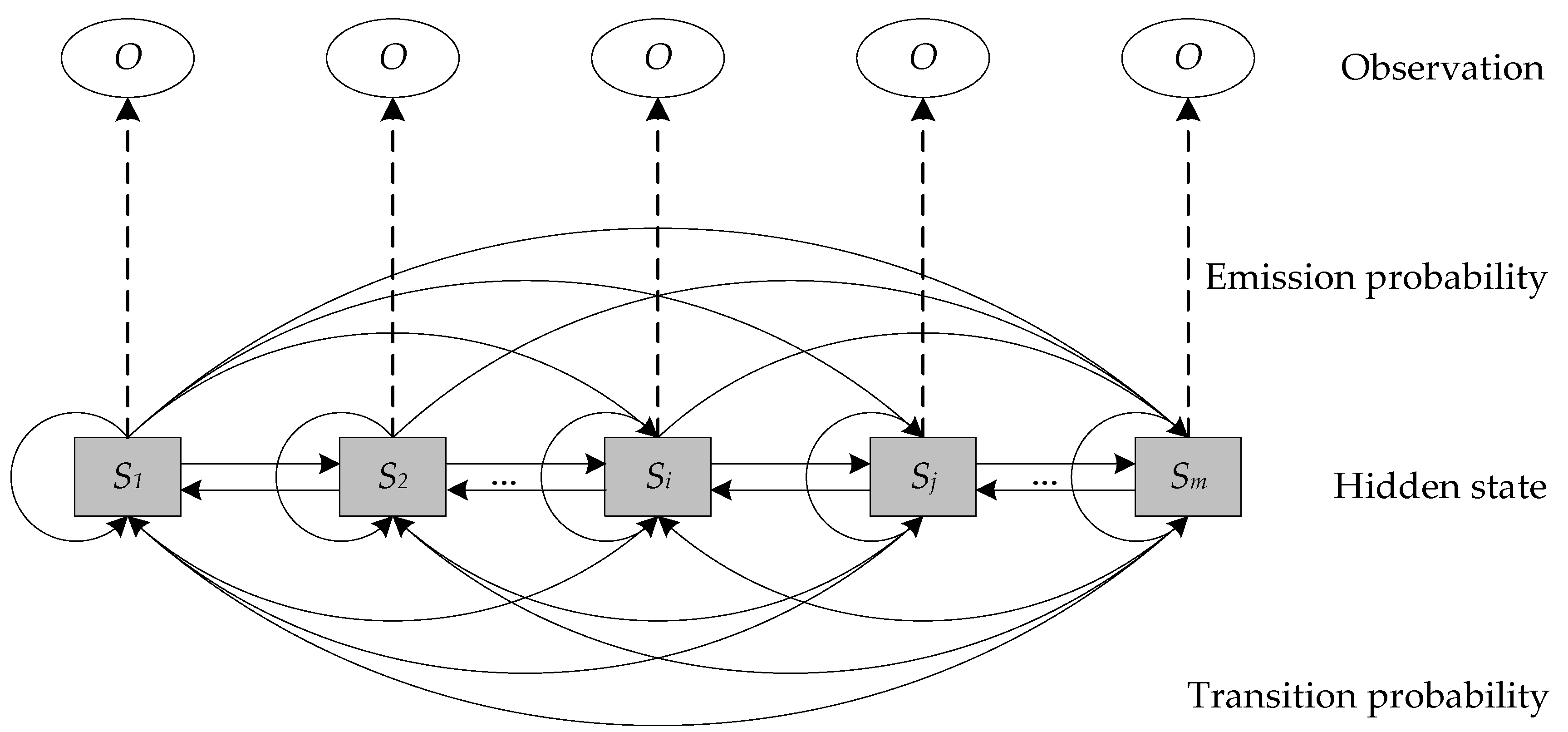
3.1.1. Hidden Markov Model

An HMM is a probabilistic model describing double stochastic processes [39] with parameters, which include Markov processes of hidden states and observation processes associated with hidden states. The process of hidden state transition is not observed directly. The change in hidden state can be inferred by observing the sequence of indexes. Objective indexes can be divided into observed variables which are convenient for direct measurement and hidden variables which cannot be directly observed. That is to say, the risk state of the hidden variable needs to be judged using observed indexes. The application of HMM can reduce the dependence on experts’ subjective experience. There is a hierarchical independent mapping relationship between these observed indexes and hidden variables. The correlation process between the hidden risk state and the observed state in the model is shown in Figure 1.

3.1.2. HMM Parameter Learning

The parameter learning algorithm is called the Baum–Welch algorithm [40], which iteratively optimizes the parameters of the HMM. Let ( ,   F ,   P ) be the probability space and { Y t } 1     t     T and { X t } 1     t     T be sequences of random variables of observable and hidden states, where X t :   S 1 , S 2 , , S m and Y t :   F N or any set of possible states.
The specific implementation steps are as follows:
Step 1: In the given sample training space, the first observation sequence y = ( y 1 , y 2 , , y T ) is trained and the initial model parameters are re-estimated to obtain the model parameters λ 1 = ( π 1 , A 1 , B 1 ) , where π 1 stands for the distribution of hidden states, A 1 is the transition probability matrix, and B 1 represents the distribution of observable states.
Step 2: The observation sequence y = ( y 1 , y 2 , , y T ) is trained using the new re-estimated parameters λ 1 = ( π 1 , A 1 , B 1 ) to obtain the next new model parameters λ 2 = ( π 2 , A 2 , B 2 ) .
Step 3: Step 2 is repeated until the model converges. Using the three re-estimation equations mentioned below, the initial parameters of the HMM model are updated from λ 0 = ( π 0 , A 0 , B 0 ) to λ = ( π , A , B ) , satisfying P ( y | λ ) P ( y | λ 0 ) .
The parameter re-estimation equations are as follows.
π = γ 1 ( i ) = α 1 ( i ) · β 1 ( i ) i = 1 m α 1 ( i ) · β 1 ( i ) .
a t ( i , j ) = ξ t ( i , j ) γ t ( i ) .
b i ( y t ) = α t ( i ) · β t ( i ) i = 1 m α t ( i ) · β t ( i ) .
In Equation (1), π is the estimation of initial probability π , and it stands for the probability of the hidden risk state S i at time t = 1; α t ( i ) represents the forward probability function of the observation O = ( y 1 , y 2 , y t ) at time t in state i, and β t ( i ) stands for the backward probability of the partial observation sequence from time step t + 1 to the end. In Equation (2), a t ( i , j ) is the estimation of state transition probability a t ( i , j ) , and it stands for the quotient of frequency of the risk state transition from state S i to S j divided by the frequency of the hidden state transition from state s i to others; ξ t ( i , j ) = P ( X t = S i | X t + 1 = S j )   is the probability of being in state S i at time t and state S j at time t + 1, while γ t ( i ) = P ( X t = S i )   is the probability of being in state S i at time t. In Equation (3), b i ( y t ) is the estimation of observation probability b i ( y t ) , and it stands for the quotient of frequency of the observed state O i from hidden state S i divided by the frequency of observation from the hidden state S i .

3.2. The Application of Hidden Markov Model

3.2.1. Description of Bauxite Shipping

● Process Risk
The process risk is a dynamic characterization of the risk state at any time during the system’s operation. It is the output of the coupling effect of uncertain (random) events under the influence of risk factors [41]. The process risk of bauxite shipping describes the development and evolution of the bauxite shipping system between the safety and accident subsystems of Handy bauxite carriers, where bauxite continuously interacts with the traffic environment over time.
● Risk performance
The risk performance indicates the general status of the risk at a particular time, as well as the properties and characterization of the mechanism of the risk variation. The performance introduced in risk research highlights the temporal processes and spatial spread. Based on the severity of consequence and response, the risk performance of a process is quantified and classified as normal, medium, high, or uncontrolled. The responses of the four-state sequence are undesired intervention, partial intervention, consistent intervention, and invalid intervention, respectively.

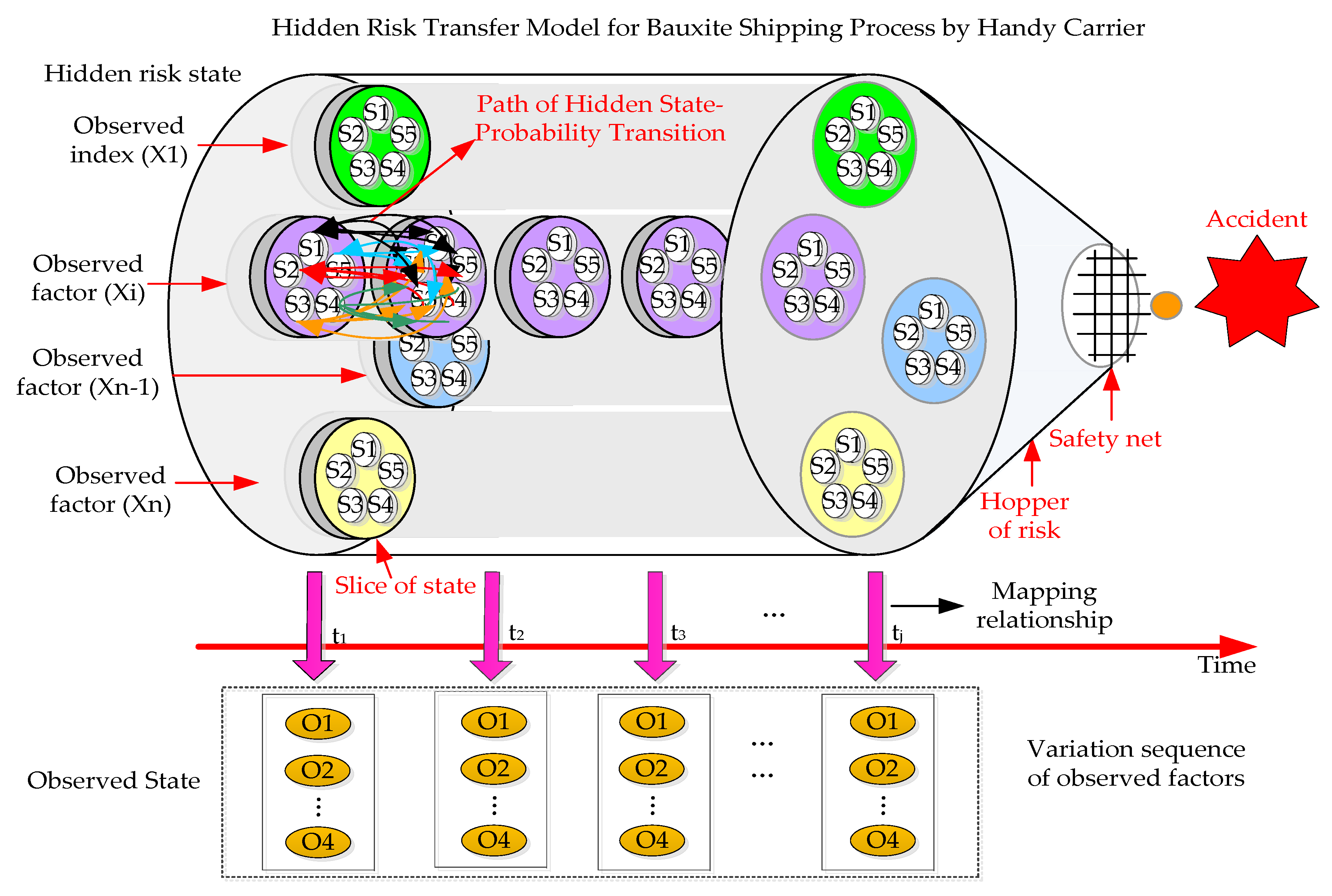
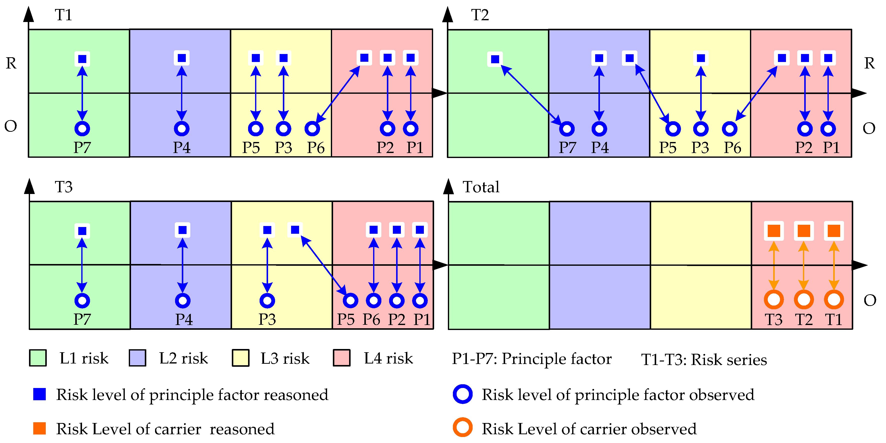
3.2.2. Risk Performance Transition of Bauxite Shipping

The factors of risk reasoning include static variables, dynamic variables, and voyage variables. Once a bauxite carrier is identified as a convenient bulk carrier, its ship parameters mostly represent static variables, such as ship age and ship technical status, while dynamic variables are environmental, such as relative length of ship (Length overall (LOA)/wavelength), wave, current, wind, and temperature. Voyage variables refer to bauxite attributes and ship maneuvering. These variables are the components of the risk evaluation system, and a change in their index values is related to the degree of system risk. However, this degree of risk cannot represent the degree of risk of the whole system. Through the risk evaluation index (observation variable), the expression of the risk state is established to indirectly show the level of total risk.
The elements in the structural model of risk reasoning for the bauxite shipping process involve objective indexes of the cargo, ship, and environment. The transition process between the risk state of the Handy bauxite carrier and the reasoning indexes constitutes an HMM. The requirements of parameter input and output in the hidden Markov model and its operation mechanism are shown in Figure 2.

3.2.3. HMM-Based Approach to Risk Performance Reasoning

The risk reasoning approach in an HMM framework can be achieved in several steps: data learning, modeling of HMM for risk reasoning, reasoning of risk performance, and performance evaluation of reasoning. The flowchart of the proposed model is shown in Figure 3.
Firstly, the risk factors of the bauxite shipping process were identified based on the accident data of “M.V Bulk Jupiter”, i.e., the Report of the Marine Safety Investigation into the Loss of a Bulk Carrier. The principal factors were obtained using principal factor analysis (PFA) from a dimensionality reduction of the risk factor set. The risk classification criteria were established after scalar quantification of the principal factors. Based on the first 50 groups of operational data of a Handy bauxite carrier, the HMM was trained using the Baum–Welch algorithm. After the steps of feature extraction, dimensionality reduction using PFA, and scalar quantization, the last nine groups of operational data were input as test data into the HMM to obtain the log-likelihood probability, which was then used for similarity recognition and risk performance reasoning. Then, the reasoned risk performance of each factor was compared with the test data from the last nine groups to evaluate the performance of risk reasoning in terms of classification effectiveness, measurement accuracy, and reasoning sensitivity.

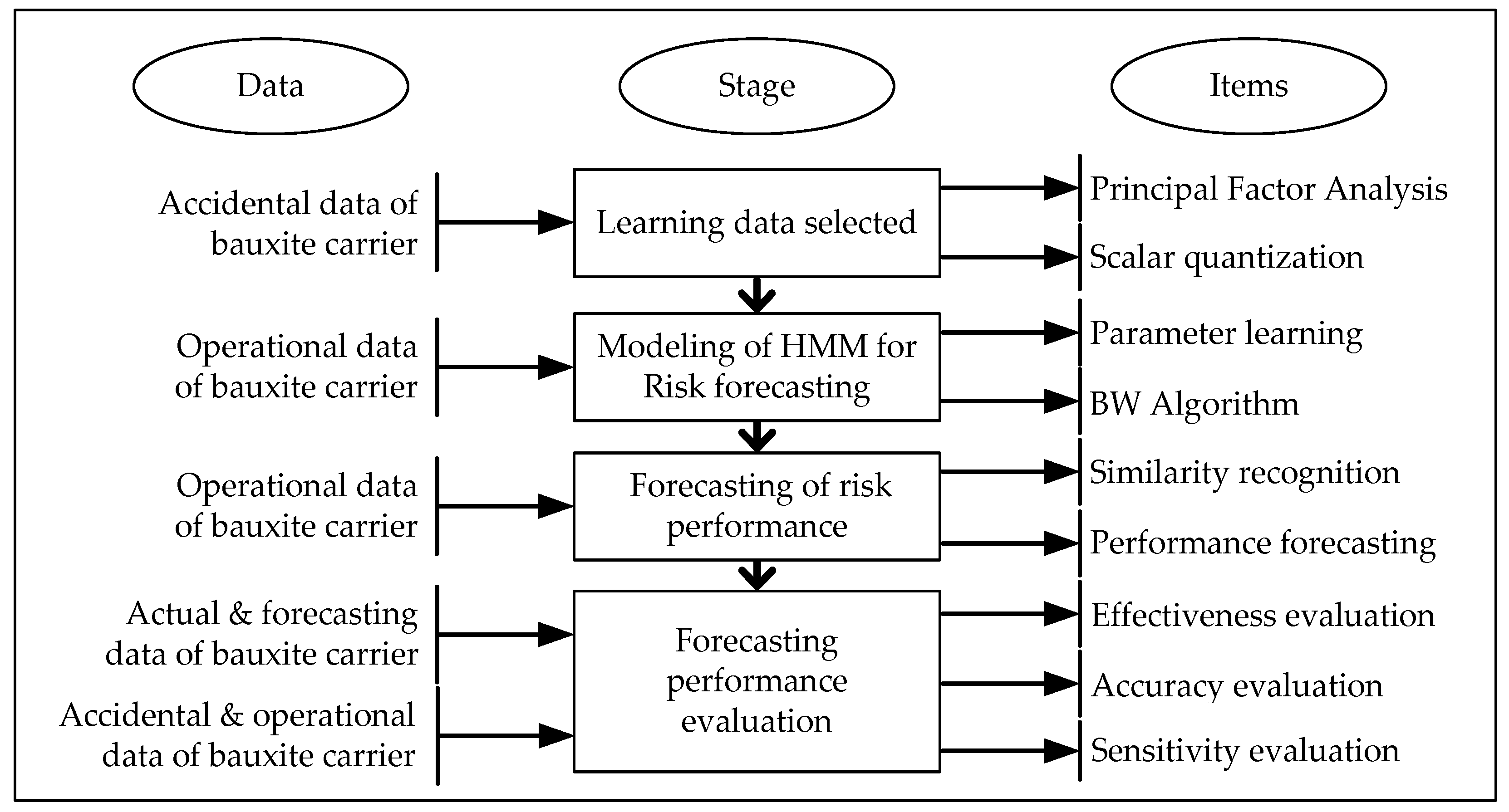
3.3. Modeling of HMM for Risk Performance Reasoning

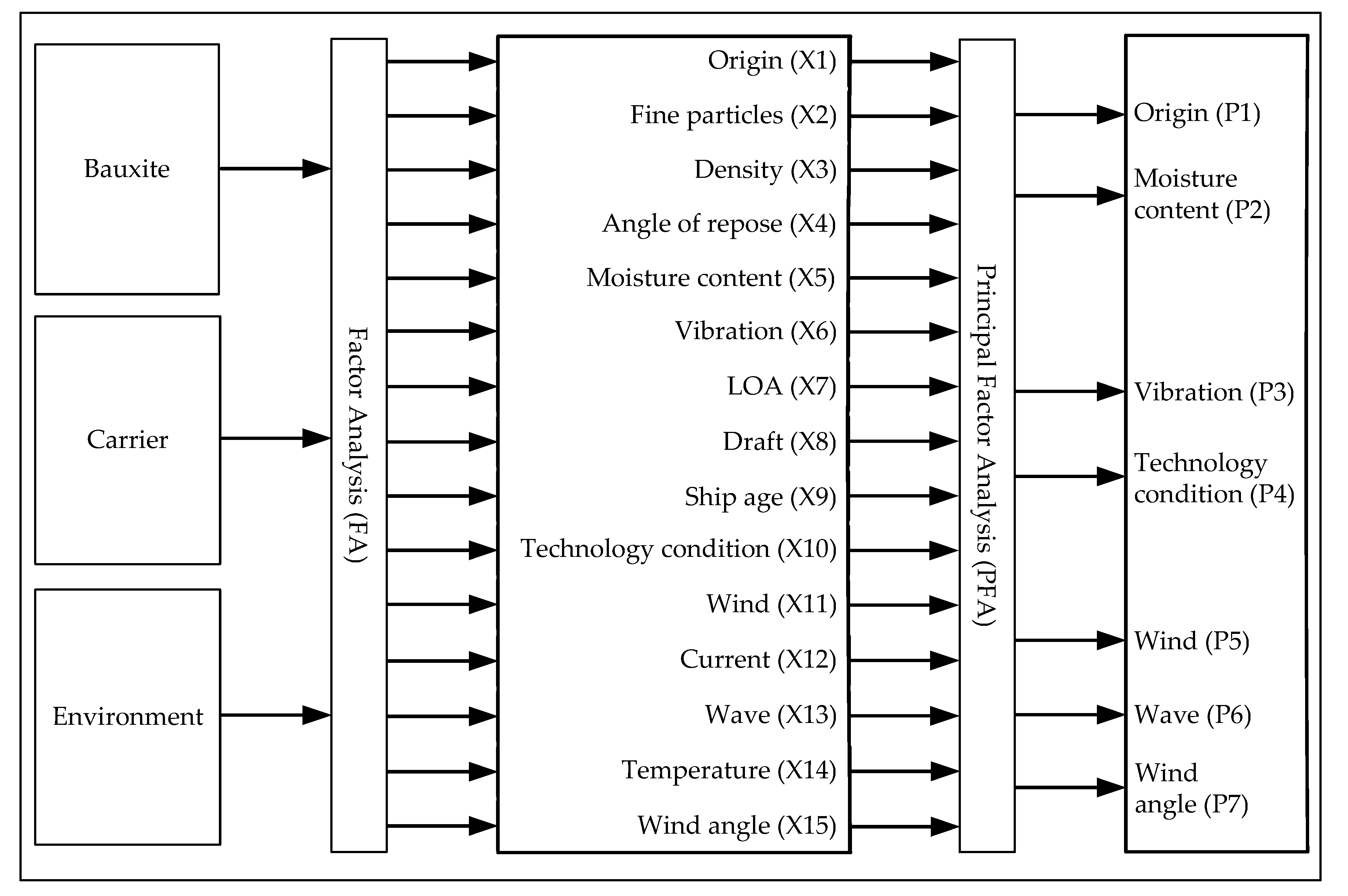
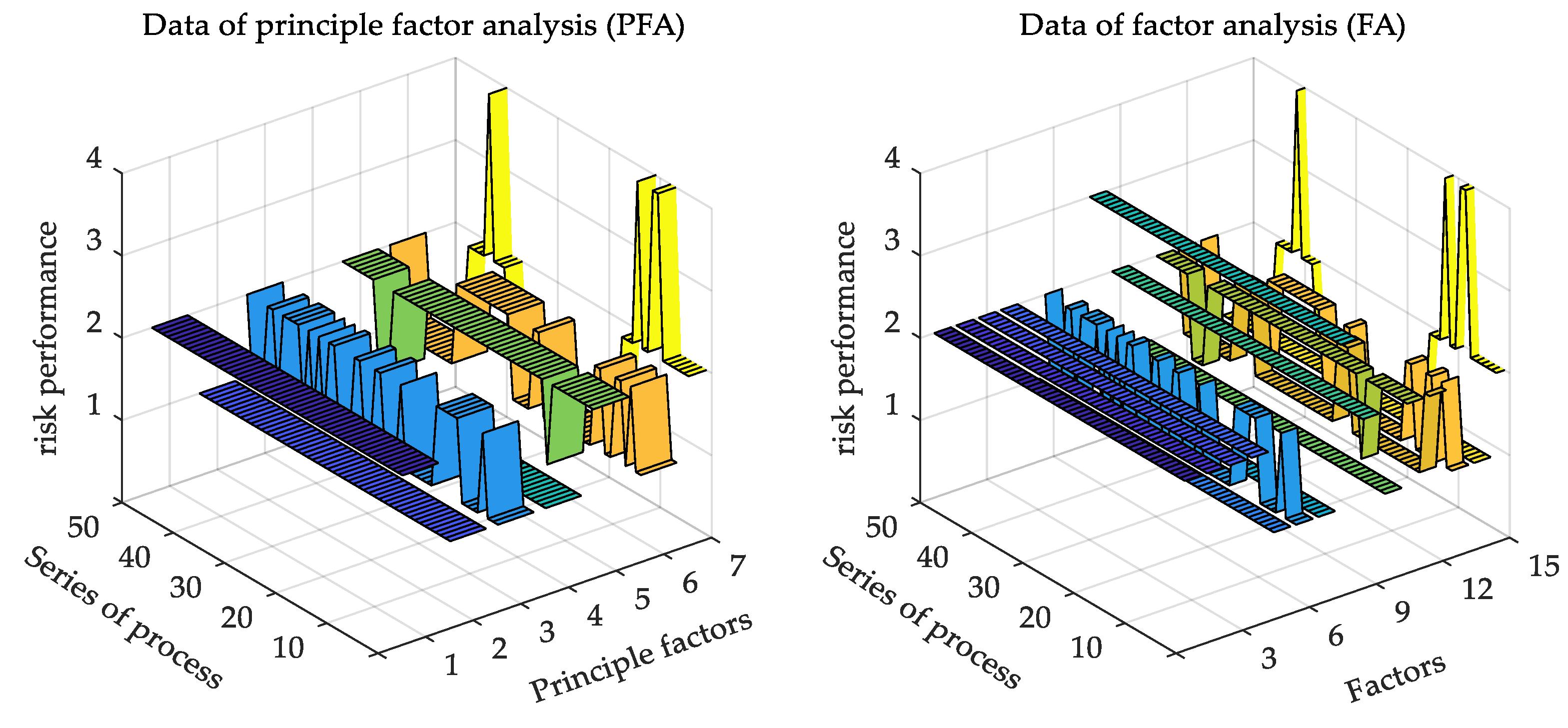
3.3.1. Principal Factor Analysis

Based on the risk identification of the risk of bauxite shipping process, a total of 15 risk factors (RFs) were obtained for the three types of factors: bauxite, Handy carrier, and environment. After experimental analysis of the coupling effect of the bauxite and Handy carrier under complicated marine conditions, seven principal factors (PF) were selected from the RFs, including static factors, voyage factors, and dynamic factors, for risk reasoning of the bauxite shipping process. System of principal factors is present in Figure 4.

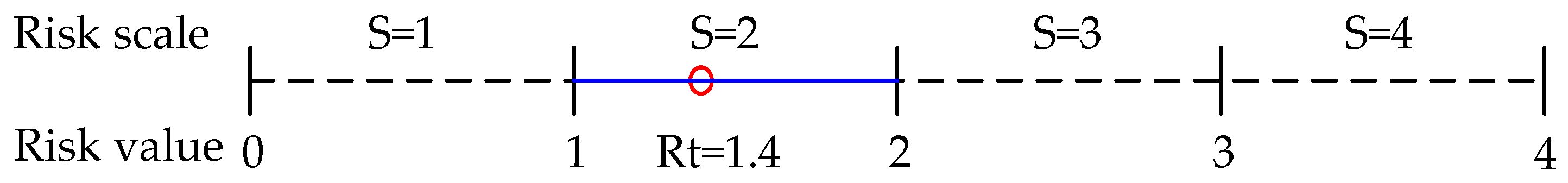
3.3.2. Scalar Quantization

● Factors and classification criteria
With the rapid development of big data, much more information in maritime safety needs to be processed quickly. Studies on the quantitative risk analysis of ships are becoming more important [42]. Quantifying the factor values that can characterize the risk performance is helpful to explain their impact on the bauxite shipping process. In order to facilitate the application of the original data in the hidden Markov reasoning model, continuous values are discretized [43] and the risk grade is divided by the interval value for the quantitative factors. The other qualitative factors can be transferred into grades, as shown in Table 1.
Here, the range of risk grade values is based on the consideration of facilitating seafarers to classify and control the aforementioned risk indexes. Considering the complexity of ship maneuvering, it is difficult to accurately determine the risk level in the risk range of continuity for crews. For example, clear risk guidance is necessary for emergencies in Beaufort 8 wind. Although the risk level of the index changes when the actual index value is at the critical value of the adjacent risk level, the variables are still insufficient to achieve the degree of mutation in the total risk reasoning. When the risk level is very high, a sudden change in some key indexes may lead to a significant increase in the total risk of the ship, which highlights the need to control disaster-causing factors in bauxite shipping.
● Quantization regulation of factors of risk performance
Based on the risk scale criteria of principal factors, each grade risk is defined as a standard value of 1–4, representing normal, low risk, high risk, and uncontrolled risk, respectively. After the total risk value is obtained by quantization and combination of the risk performance of principal factors, the total risk scale can be obtained by scalar quantization. The risk value belonging to any risk scale interval can be defined as the standard value of risk. When the total risk value R t ϵ ( i ,    i + 1 ] , then we accept its risk scale S t = i + 1 at moment t, where 0 < i < N , 1 t T (see Figure 5).

3.4. Risk Performance Reasoning

3.4.1. Similarity Recognition

HMM parameters were trained using actual data of Handy bauxite carriers under normal conditions, representing a better cargo state, satisfactory ship conditions, and a good environment. Similarity recognition was performed using the Viterbi algorithm to obtain the maximum of log-likelihood probability, which is expressed as follows:
L L P t = log P ( Y t = O | λ ) ,
where L L P t is the log-likelihood probability of the observations { Y t } at the current time t under the HMM of λ .
The next step is to detect the closest L L P t 0 from the L L P t m a x of the historical data and obtain the risk performance at time t 0 . This function is expressed as follows:
D i f f ( L L P t ) = | log P ( Y t = O F t | λ ) log P ( Y t = O H | λ ) | ,
where D i f f ( L L P t ) is the difference between log P ( Y t = O F t | λ ) and log P ( Y t = O H | λ ) , log P ( Y t = O F t | λ ) indicates the max log-likelihood probability of the forecasted O at the current time t under the HMM of λ , and log P ( Y t = O H | λ ) expresses the log-likelihood probability of the historical O at the under the HMM of λ .
The series of D i f f ( L L P t ) was sorted in ascending order by the MATLAB function “[LLsort, LLpos] = sort []”, from which the original element position was returned. Given n as the number of steps, the n closest L L P t 0 was obtained based on the n smallest D i f f ( L L P t ) .
The above approach is called similarity recognition.

3.4.2. Risk Performance Reasoning of Factors

For each principal factor, the difference between the current risk value and the next reasoned value is the same as the difference between the two adjacent risk values discovered using similarity recognition. The reasoned value at time t + 1 can be obtained from the former risk value. The approach can be expressed as follows:
{ F 1 H K = 1 N n = 1 N ( H k + 1 ( n ) H k ( n ) ) ,      k [ 1 , K 1 ]   F t F t 1 = 1 N n = 1 N ( H k + 1 ( n ) H k ( n ) ) ,     t [ 2 , T ]
where T is the length of series reasoned, K is the length of historical series, N is the number of the closest LLP of HMM for the carrier at the current time, F 1 is the first value, H K is the last historical risk value which is also the benchmark of risk reasoning, F t is the risk value reasoned at time t , F t 1 is the risk value reasoned at time t 1 , H k ( n ) is the n closest historical risk value compared with the L L P t of the benchmark and F t 1 , H k + 1 ( n ) is the next historical risk value of H k ( n ) .
Nevertheless, it must be noted that, if F 1 H K > 0 , then the reasoned (forecasted) risk value F t grows linearly at every moment based on Equation (6); therefore, the output of every step is normalized using the quantization regulation.

3.4.3. Risk Performance Reasoning of Ship

The reasoned risk value of principal factors and the total risk value were set as intervals of the risk state value ranging from 0–4. The risk performance of principal factors was reasoned through a quantization of the risk grade using scalar quantization regulation. The quantization regulation of the risk performance can be used to gain the total risk performance reasoning at any future time.
Reg. 1: when the risk grade of the moisture content (K2) is 1, that is, S K 2 = 1 , the total risk value of the bauxite carrier is R t = A v e r a g e ( S K 1 : S K 7 ) , and then the total risk grade S t can be obtained using quantization regulation.
Reg. 2: when the risk grade of K2 is 2, that is, S K 2 = 2 , and the risk grade of vibration (K3) or wind (K5) is between 2 and 3, that is, 2 (   S K 3   o r   S K 5 ) 3 , the total risk value of the bauxite carrier is S t = m a x ( S 3 , A v e r a g e ( S K 1 : S K 7 ) ) .
Reg. 3: when the risk grade of K2 is 2, that is, S K 2 = 2 , and the risk grade of K3 or K5 is between 2 and 3, that is, S K 3   o r   S K 5 = 4 , the total risk value of the bauxite carrier is S t = m a x ( S 4 , A v e r a g e ( S K 1 : S K 7 ) ) .
Reg. 4: when the risk grade of K2 is 3, that is, S K 2 = 3 , the total risk value of the bauxite carrier is S t = m a x ( S 3 , A v e r a g e ( S K 1 : S K 7 ) ) .
Reg. 5: when the risk grade of K2 is 4, that is, S K 2 = 4 , the total risk value of the bauxite carrier is S t = m a x ( S 4 , A v e r a g e ( S K 1 : S K 7 ) ) .

3.5. Performance Evaluation of Reasoning

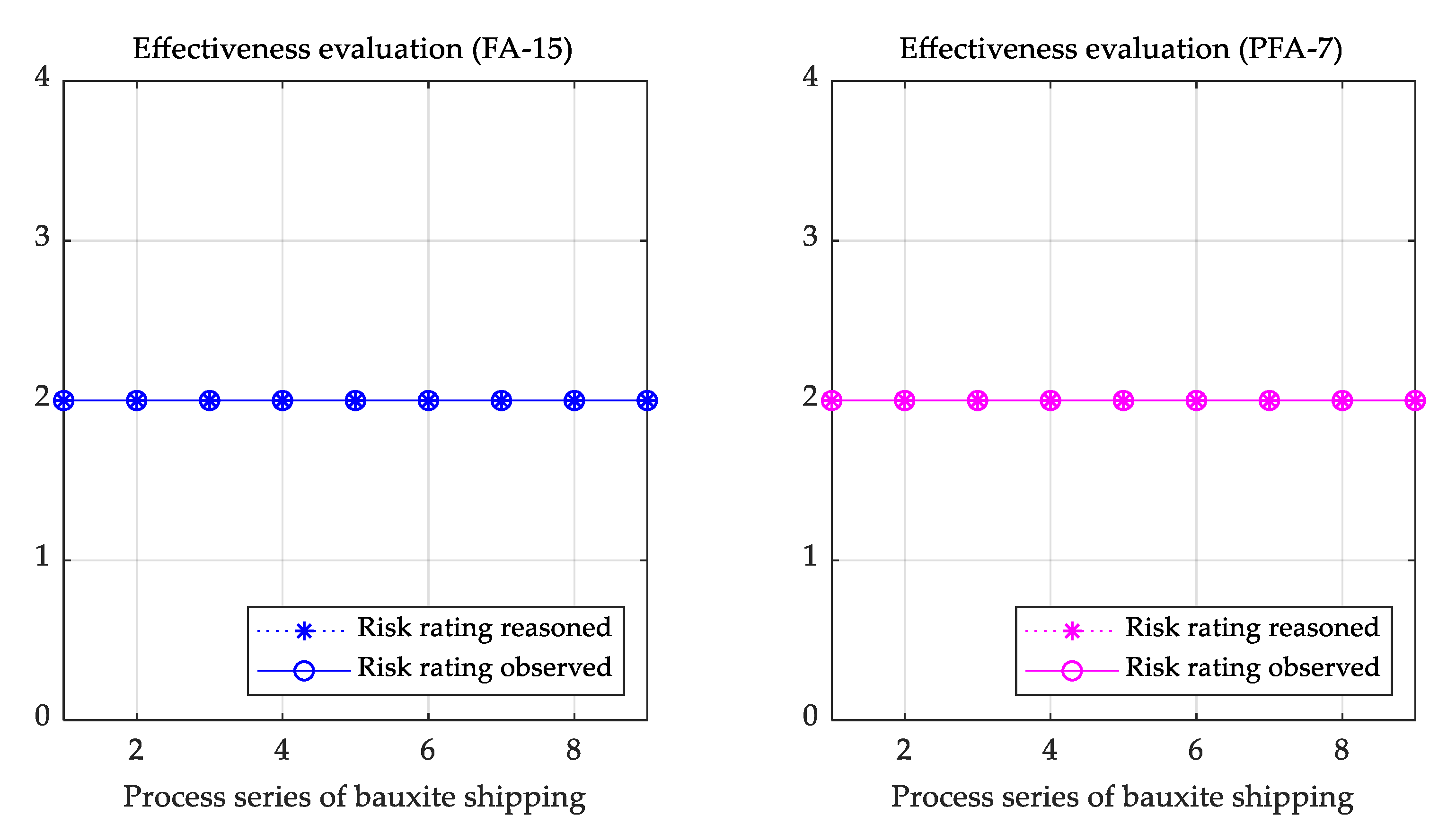
3.5.1. Effectiveness Evaluation

The effectiveness evaluation of the risk performance reasoning can be expressed using the degree of bias (DOB) and degree of detection (DOD), defined as follows:
DOB = F i j F j i = i = 1 4 ( f i j f j i ) T ,
DOD = F i i F j i = i = 1 4 ( f i j f j i ) T ,
where i and j denote the ordinal values of the risk category, satisfying i   a n d   j   ( 1 , 2 , 3 , 4 ) ; T is the length of series to be reasoned, and F i j is the relative frequency of the forecast risk category i while the observed risk category is j (a non-i interger value), which can be calculated as the count of f i j occasions in all four risk categories divided by the length of the reasoned series. F j i can be similarly obtained. F i i is the relative frequency of the forecast risk category equal to the observed risk category i which can be calculated as the count of f i i occasions in all four risk categories divided by the length of the reasoned series.
The degree of bias compares the number of times a risk category was forecast to the number of times the risk category was observed. It indicates that the forecast categories were over-forecast or under-forecast with a value greater or less than 0, respectively, while a value of 0 describes unbiased forecasts. The degree of detection is the fraction of occasions when the risk forecast category occurred for occasions when it was also forecast. This value represents the success rate for detecting different risk categories and ranges from −1 as completely wrong to 1 as completely accurate.

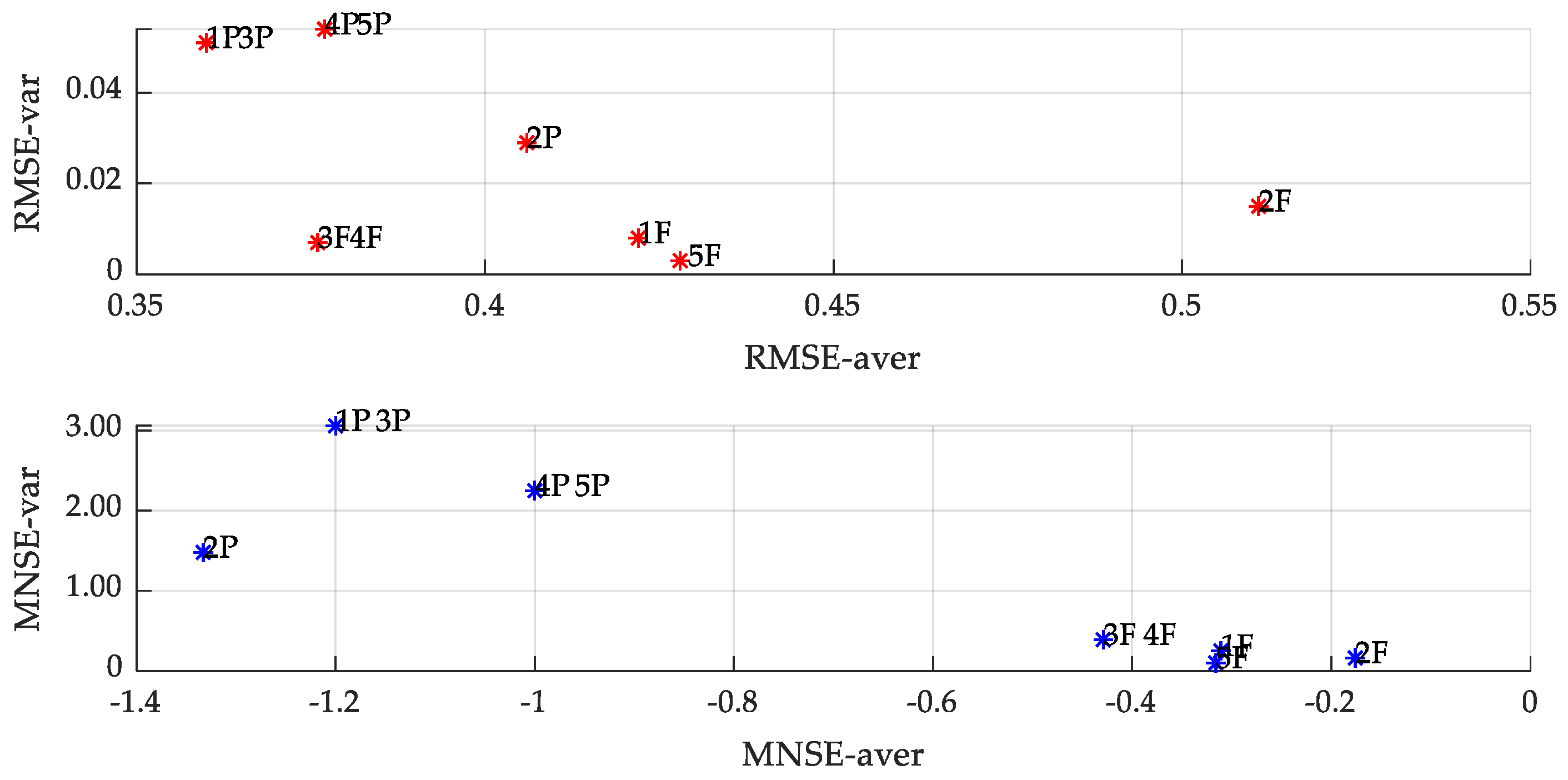
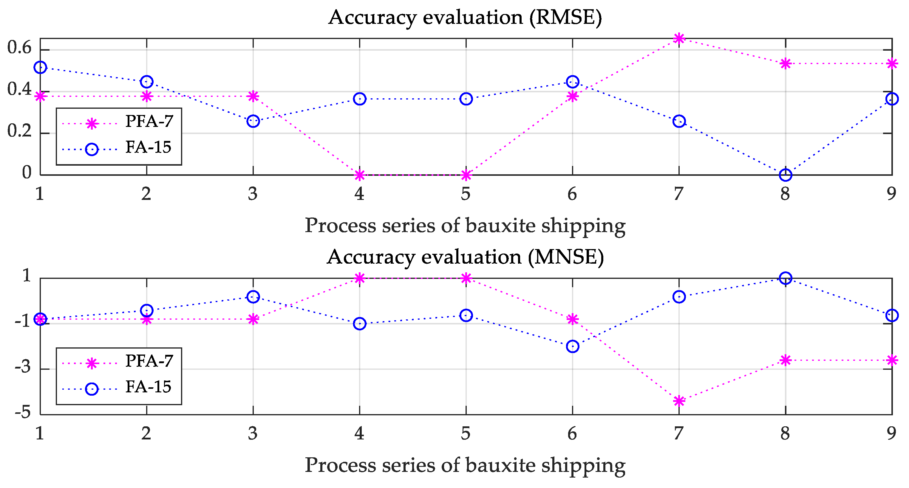
3.5.2. Accuracy Evaluation

The accuracy evaluation of the risk performance reasoning is expressed using the root-mean-square error (RMSE) and modified Nash–Sutcliffe model efficiency coefficient (MNSE) [36], defined as follows:
RMSE = 1 T t = 1 T ( O ( t ) F ( t ) ) 2 ,
MNSE = 1 t = 1 T ( O ( t ) F ( t ) ) 2 t = 1 T ( O ( t ) O ¯ ) 2 ,
where O ( t ) and O ¯ are the observations and the mean values of the observations, respectively; F ( t ) stands for the reasoned values, while T is the length of series to be reasoned.
RMSE is mainly used to represent the standard deviation of the differences between observations and forecasts. The range of the RMSE lies between 0 and infinity. A value of 0 for the RMSE indicates that the forecasts are as accurate as the mean of the observations, while bigger values show that the reasoning model is worse than the observed expectation.
MNSE is used to measure the evaluation accuracy and is defined as one minus the sum of the absolute squared differences between the observed and reasoned values divided by the sum of the absolute squared differences between the observations and observed expectation. The range of the MNSE lies between negative infinity and 1.0 (perfect match). A value of 0 for MNSE denotes that the value reasoned is the same as the observed expectation, while negative values for MNSE show that the reasoning model is worse fitted to the observation or explains relationships poorly compared to the model defined using the mean value of observations.

3.5.3. Sensitivity Evaluation

The data from the simulation scenarios and the accident scenario were used for a sensitivity evaluation to judge the deviation of those scenarios from the normal state of bauxite shipping. The deviation of the HMM-based risk reasoning approach is defined as the degree of sensitivity (DOS), which is modified from the concept of the discrete degree of classification [44], in order to avoid invalid measurements due to some LLPs being minus infinity. DOS is expressed as follows:
DOS i = 1 2 × ( log P m a x ( O i | λ ) log P m a x ( O 0 | λ ) log P m a x ( O i | λ ) + log P 2 n d   m a x ( O i | λ ) log P 2 n d   m a x ( O 0 | λ ) log P 2 n d   m a x ( O i | λ ) ) × 100
where log P m a x ( O 0 | λ ) and log P 2 n d   m a x ( O 0 | λ ) are the maximum and the secondary maximum of LLP under the HMM of the normal scenario, respectively, while log P m a x ( O i | λ ) and log P 2 n d   m a x ( O i | λ ) are the maximum and the secondary maximum of LLP under the HMM for the i scenario, respectively. Furthermore, the maximum and the secondary maximum of LLP are the first and second values of the LLP series listed in descending order.
DOS ranges from 0 to 100. As DOS approaches zero, the total performance becomes more normal. A greater DOS value denotes greater deviation of the risk performance from the normal.

4. Results

4.1. Data of Handy Bauxite Carrier

4.1.1. Ship Parameters

In order to verify the approach to risk performance reasoning, two Handy bauxite carriers were selected: one still in service, and another which previously sank. Their general parameters are listed in Table 2.

4.1.2. Operational Case

The No. 1509 voyage of M.V. Yuming carried bauxite from Guandan Port, Malaysia, on 28 July 2015. The weather at the loading port was fine a few days before arrival and during the loading period. It took 10 days to reach the destination port of Laizhou, China. There was no water leakage in the sewage well during the voyage of the ship, and the actual performance of the cargo was stable. The annual mean wave height is 1.62 m and the average wave period is 6.62 s in the waters of the Taiwan Strait [45]. Here, 94% of the wave lengths are less than 100 m, and 15% of them are between 70 and 100 m. During the voyage, the weather was good, the visibility was medium, the pressure was stable, the temperature was 20–32 °C, and the meteorological wind and wave levels were 3°–4°. Wind direction was mostly in the bow and stern direction. Except for the first day when the wind pressure difference was as high as 7°, the voyage flow pressure difference did not exceed 3°.

4.1.3. Accident Case

M.V. Bulk Jupiter sailed from Guantan Port, Malaysia, to Qingdao, China. During the loading period, the eastern coast of Malaysia suffered record-breaking rainy weather. The loading operation was delayed repeatedly due to heavy rain. Rainfall on 21 and 23 December during the subsequent loading periods was as high as 240 mm and 258 mm, respectively. After consulting the accident investigation report [46], it was found that the total weight of bauxite in Bulk Jupiter’s voyage was 46,400 tons, with an average water content of 21.3%. After sailing on 30 December, the sea weather deteriorated gradually. On 31 December, the northeasterly wind was 6–7, the sea condition was 4–6, and the average wave height was 2.2 m. On 1 January 2015, the northeasterly wind was 8, while the wave height was 2.5–4 m. The swell direction was from the northeast (NE), the vessel’s route placed the sea on the port bow as the vessel sailed east-northeast on a heading of 060°. In the final moments prior to sinking, the vessel’s speed was 4.3 knots.

4.1.4. Data Collection

The factors value of time series with length of 59 were from the 4-hour interval records of No. 1509 voyage in Logbook onboard M.V. Yuming. According to the criteria of risk reasoning for Handy bauxite carriers, the risk performance rating of factors are obtained in style of PFA and FA, which is shown in Figure 6 and Figure 7. The first 15 groups of data of principle factor analysis of M.V. Yuming is set as Scenario No.1. Scenarios No.2 to No.4 are simulated conditions based on the worse cargo condition, unsatisfied ship condition and terrible environment respectively, and Scenario No.5 is an accident condition based on the last voyage of M.V. Bulk Jupiter.

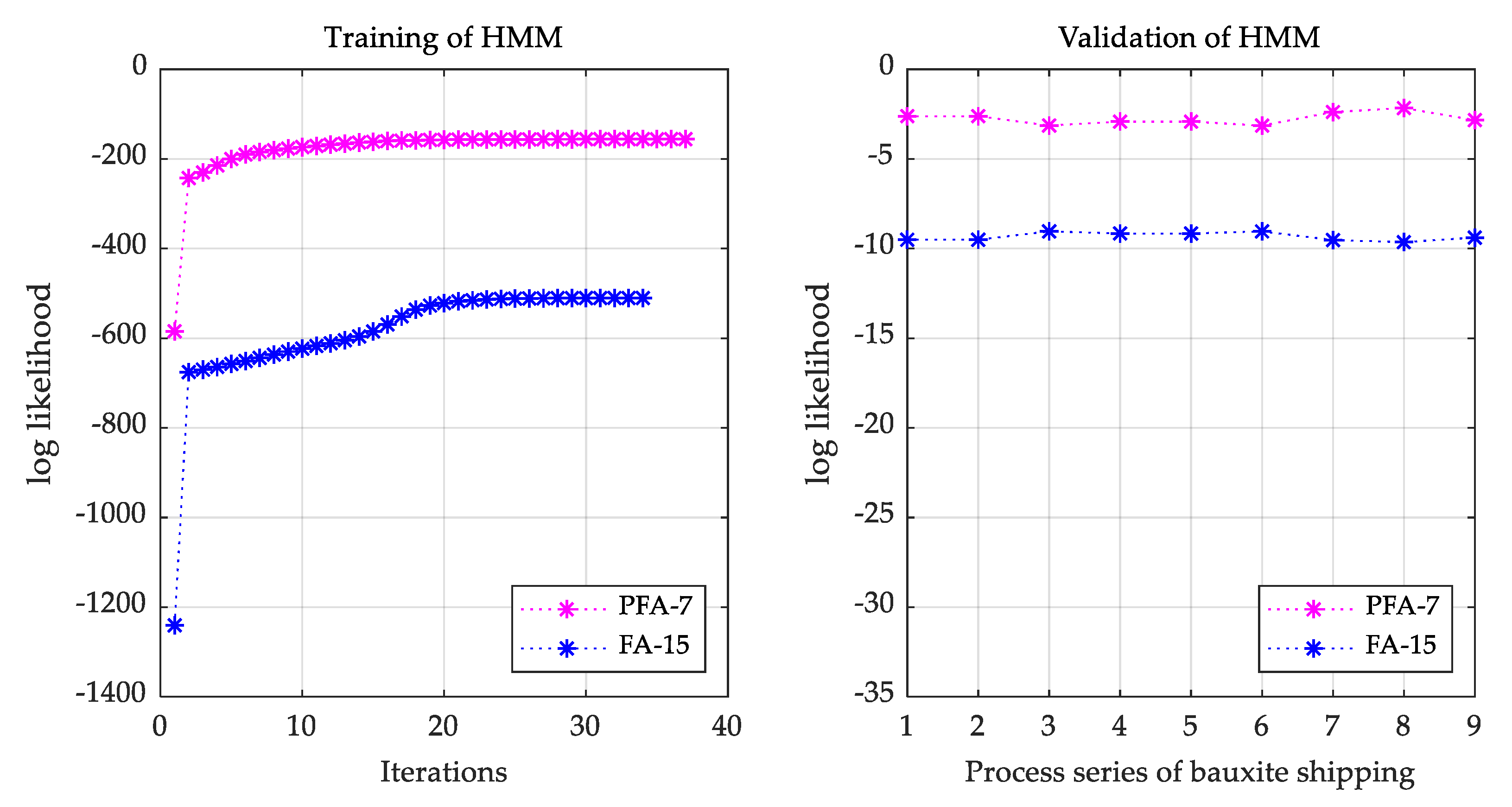
4.2. Parameter Training

The approach to selecting 15 factors for risk performance was factor analysis (FA). The approach to selecting seven principal factors for risk performance reasoning based on the bauxite model test and FA with 15 factors was principal factor analysis (PFA). Both FA and PFA were used to establish the HMM in order to reason the risk performance of bauxite shipping. In the process of parameter learning, logarithmic likelihood values were used to represent the matched degree between parameters and models. As the number of iterations increased, the matched degree tended to converge. The model parameters obtained from the training were valid because they satisfied the local optimal characteristics of the parameters.
Figure 8 indicates that the HMM tended to converge until the 37th and 34th iterations for PFA and FA, respectively. Nine groups of data were used to test the HMM and get a converged likelihood. Taking the PFA as an example, the trained and optimized HMM parameter was π = [ 1.0   0   0   0 ] .
A = [ 0.0000      0.0000      0.0000      1.0000 0.2936      0.2711      0.1408      0.2945 0.0000      0.0019      0.0000      0.9981 0.1460      0.2830      0.5710      0.0000 ] ,   and   B = [ 0.0000      1.0000           0      0.0000 0.0006      0.9994           0      0.0000 0.6020      0.3474           0      0.0505 1.0000      0.0000           0      0.0000 ] .

4.3. Selection of Approach to Reasoning

Taking the risk reasoning of M.V. Yuming as an example, the best approach to reasoning was selected as shown in Figure 9.
The RMSE values indicate that the best forecast was performed with 3K (three steps and seven principal factors). The MNSE values indicate that the best forecast was performed with 2F (two steps and 15 factors).

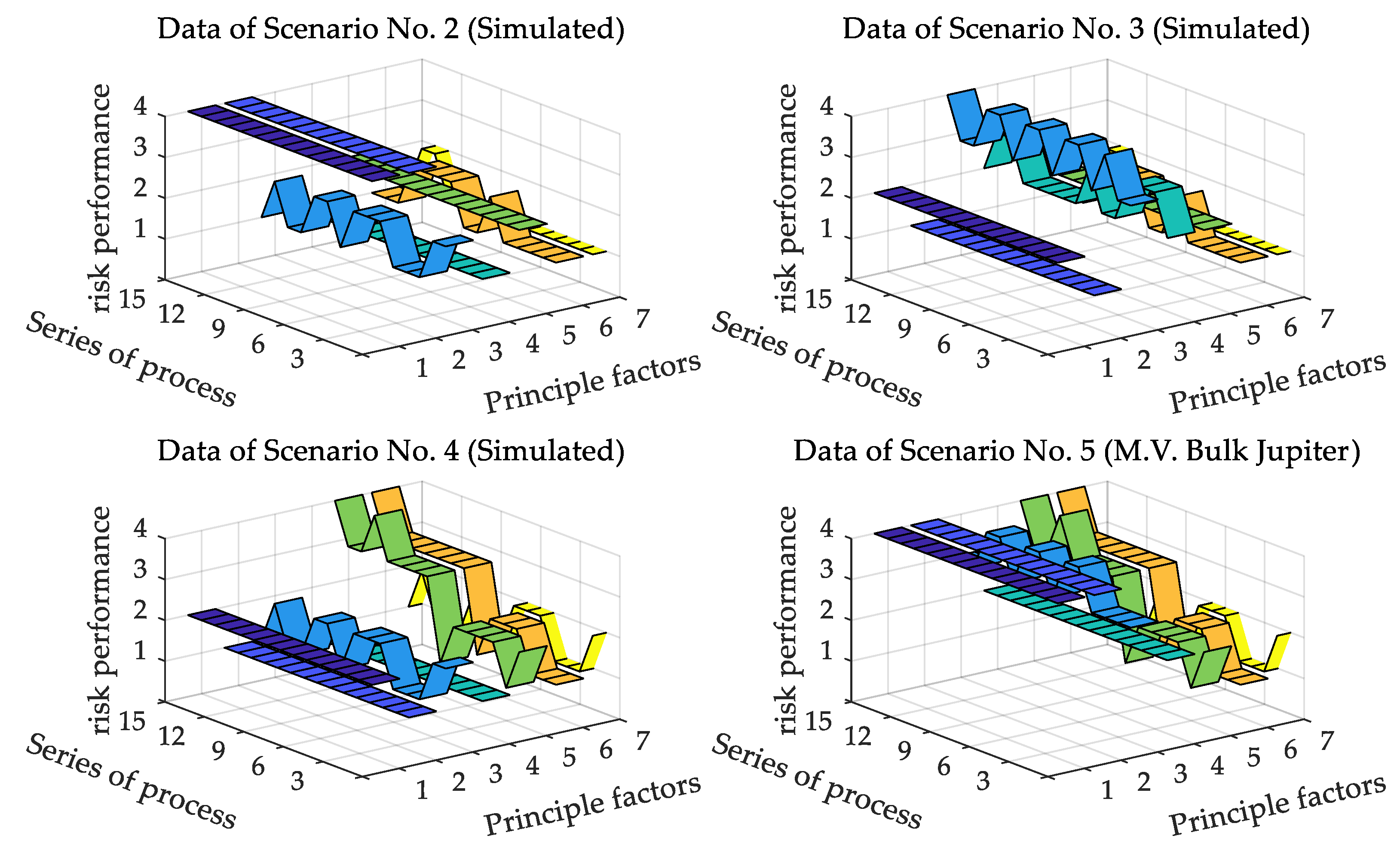
4.4. Result of Reasoning

By using the reasoning approach for the risk performance of the factors, every factor was reasoned within a risk grade boundary of 1–4. Risk grades were obtained for 15 factors (FA approach) and seven principal factors (PFA approach). According to the abovementioned quantization regulation of risk performance, the time series of the total risk performance of the bauxite shipping process was obtained. Likewise, the same approach could be used to obtain the observed sequence of the total risk performance. Taking M.V. Bulk Jupiter as an example, the risk performance reasoning model based on a three-step PFA approach was adopted. The first 12 sets of data were used to train the model parameters, and the last three sets of data were used for reasoning and testing; the results are shown in Figure 10.
The comparison with the observed risk performance shows that the reasoned risk performance with seven principal factors was mostly accurate. The risk performance of the factors was transformed into an overall risk performance using the quantification regulation. The last three periods of the whole shipping process had the highest risk rating. In fact, the accident report showed that the actual moisture content of bauxite severely exceeded the transportable moisture limit (TML), and the carrier encountered strong winds and moderate swells along the coast of Vietnam. Consequently, capsizing occurred. Therefore, the calculated risk was consistent with the actual situation. Therefore, the model constructed is effective in forecasting risk performance for the bauxite shipping process.

4.5. Effectiveness and Accuracy

Figure 11 shows the comparison of the effectiveness evaluation of reasoning using the FA and PFA approaches, where the evaluation was conducted on M.V. Yuming for the risk performance of a bauxite shipping process. It can be seen that the calculated risk rating was completely consistent with the observed risk rating, and the effectiveness of the performance reasoning was ideal. The effectiveness of the risk reasoning based on FA or PFA was also quantitatively evaluated using DOB and DOD . The degree of deviation for the risk reasoning model was DOB = 0 , indicating no deviation in the reasoning for the four risk ratings. The degree of detection was DOD = 1 , showing that the reasoned risk rating was completely accurate.
Accuracy evaluation was conducted on the calculated nine-step risk performance matrix and the actual observed risk performance matrix, as shown in Figure 12. The RMSE of reasoning based on the FA approach was 0.336 on average with a maximum of 0.516 and a minimum of 0.0, while the RMSE of the PFA approach was 0.36 on average with a maximum of 0.655 and a minimum of 0.0. The error of reasoning was small; thus, the accuracy was better evaluated. The average of the MNSE calculated using the FA approach was −0.459, ranging from 1.0 to −2.0. The average of the MNSE calculated using the PFA approach was −1.20 with a maximum of 1.0 and a minimum of −4.40. The MNSE values based on the two approaches were slightly smaller than zero; therefore, the reasoned performance was slightly conservative due to the values being lower than the actual risk performance.

5. Analysis and Discussion

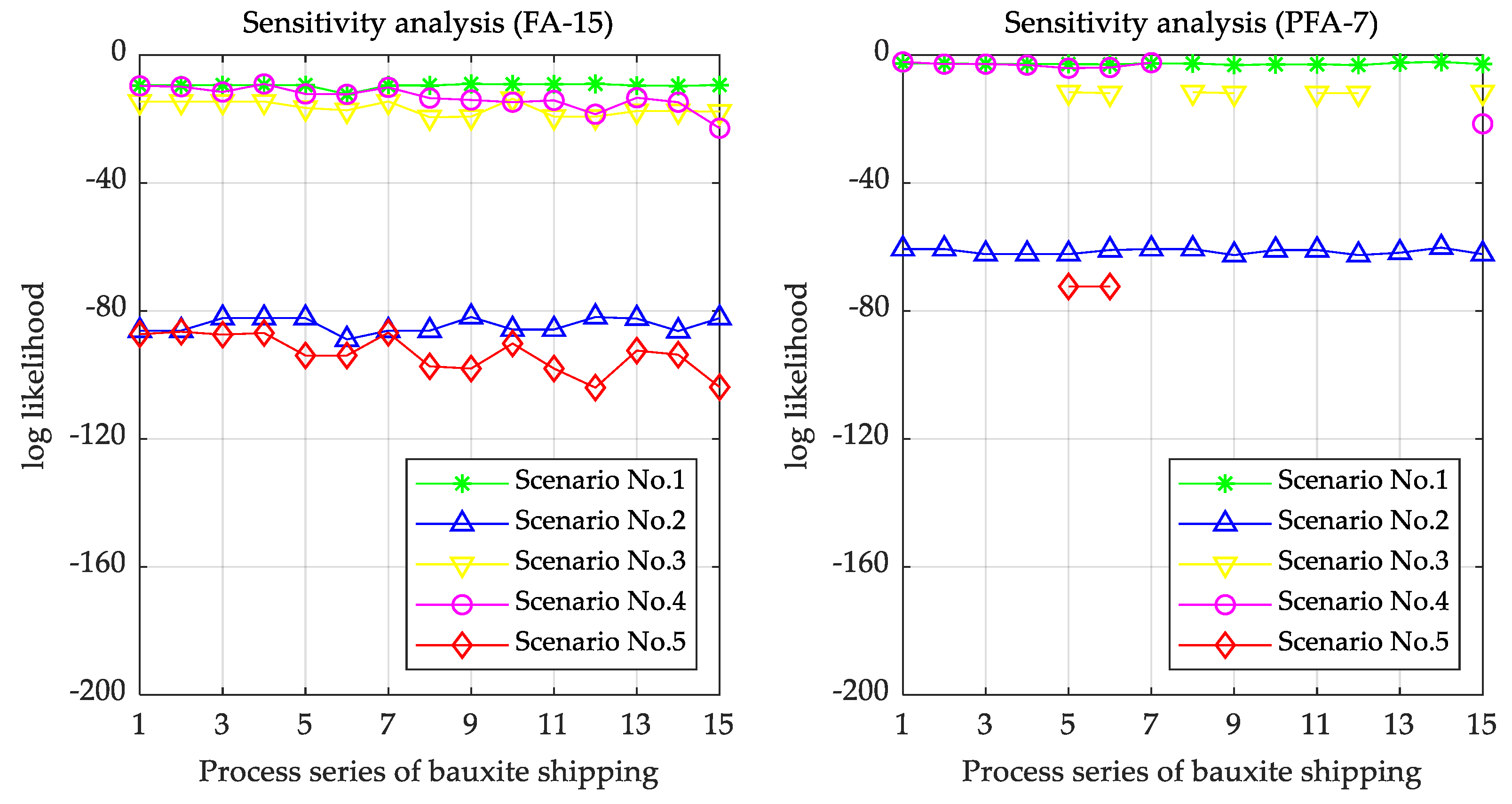
5.1. Sensitivity Analysis

Five groups of test data of the bauxite shipping process were selected for sensitivity evaluation. Scenario No. 1 featured normal conditions based on the No. 1509 voyage of M.V. Yuming. Quantitative analysis was carried out on the conformity of risk performance under each scenario. The sensitivity function of the risk reasoning model established previously was used to obtain the degree of sensitivity (DOS) for each scenario relative to normal scenario No. 1.
Table 3 indicates that the effects of scenarios No. 2 and No. 5 were relatively close, representing the worst risk performance deviated from the normal scenario for bauxite shipping. Compared with the FA-based DOS, the PFA-based DOS was more sensitive. The risk assessment and classification of scenarios No. 2 and No. 5 were the best, with sensitivity values above 95, meaning that any abnormal risk performance of bauxite shipping can be detected more accurately. The sensitivity of scenario No. 4 was very small, showing that the model could not effectively distinguish the risk performance of bauxite shipping using the benchmark model. When the environment was poor, the risk performance of scenario No. 4 was consistent with that of normal scenario No. 1, and the risk was very low.

5.2. Pre-Warning of Threat

The risk performance reasoning model constructed in this paper is based on the normal conditions of cargo, ship, and environment for Handy bauxite carriers. The data of factors for scenarios No. 2 to No. 5 were input into the HMM for risk performance reasoning based on Scenario No. 1, where the log-likelihood probability of the output could provide a guide to abnormal risk monitor. A larger log-likelihood would denote a greater probability of low risk performance. Figure 13 demonstrates the log-likelihood value of 15 time series for scenarios No. 1 to No. 5.
The logarithm likelihood values of scenario No. 3 with unsatisfactory ship conditions and of scenario No. 4 with a terrible environment were close to those of the normal scenario No. 1.
The log-likelihood value of scenario No. 2 with worse cargo conditions more obviously deviated from that of scenario No. 1 than that of Scenario No. 3 and Scenario No. 4, indicating that the risk performance of the Handy bauxite carrier in scenario No. 2 was worse, and that the deterioration of cargo with respect to ship conditions and the environment had a greater impact on the total safety of the bauxite shipping process.
Scenario No. 5 had a more serious deviation from the normal condition. This deviation was more significant than the worst scenario of single-category factors such as the cargo, ship, or environment, which all contribute to the total risk of bauxite shipping process. It was found that the coupling effect of risk factors produced a coupling risk, which aggravated the total risk performance during the shipping process.
When using the PFA-based risk reasoning model to detect the performance, the log-likelihood value of individual time points was negative infinite, indicating that the risk behavior at this time was seriously inconsistent with the normal scenario. The risk performance at this time point can be determined as the highest rating, which is unacceptable.
In scenarios No. 3, 4, and 5, the log-likelihood probability decreased gradually, showing that the total performance deviated from the normal condition and deteriorated gradually, thereby achieving the state monitoring and issuing a pre-warning threat during the shipping process.

5.3. Risk Performance Reasoning with Hidden Markov Model

  • The influencing factors of the reasoning performance were obtained through the demonstration, thereby providing a reference for optimizing the model parameters and the reasoning approach. According to the results and analysis of the risk performance reasoning, increasing the training data and identifying principal factors can improve the reasoning performance.
  • Due to the great influence of cargo performance on the total risk performance of Handy bauxite carriers, high-risk cargo factors should be avoided. In particular, when the size of a bauxite carrier and the shipping environment or ship routing cannot be changed, the cargo quality related to shipping safety must be closely monitored, and a moisture content audit must be performed before loading, while rainproof measures should be ensured during loading and navigating.
  • Compared with the effect of any single factor, the effect of the cargo, ship, and environment is more significant, leading to a transition of the total risk performance of Handy bauxite carriers. The process between subsystems is an important part of the shipping process risk control of Handy bauxite carriers. In order to ensure safety of shipping, it is essential to respond to risks timely and effectively based on accurate multi-source risk data, such as ship maneuvering, environmental information, and dynamic cargo information from the water ingress alarm system and the radar fluid-level meter fixed in the cargo hold. Therefore, it is essential to make full use of the Internet of things and artificial intelligence to develop intelligent risk monitoring sensors and forecasting equipment for shipping processes on Handy bauxite carriers.
  • Based on the accurate historical data of principal factors and a more detailed classification of risk performance, short-term process risk reasoning with high-quality can be realized. Detailed shipping data of bauxite and Handy carriers include, but are not limited to, information from the logbook, which can be used in parameter learning to obtain more accurate parameters of the HMM. This will allow real-time monitoring and pre-warnings of cargo liquefaction and ship stability for the navigator onboard and ship manager ashore.
  • In total, 91% of the accidents on international routes caused by the liquefaction of solid bulk cargo involve Handy carriers [47], which are usually between 80 m and 190 m in length. When a Handy carrier navigates at sea with a wavelength of 90–150 m and the speed is close to the wave speed, the ship ends up hogging and sagging, threatening the structural strength of the ship. The stability of the ship is, thus, greatly reduced.
  • If possible, Handy carriers with bauxite should avoid sailing in heavy seas. In the stormy season, some special voyages of bauxite shipping could be conducted by larger bulk carriers or special ore carriers, which would have strong stability even when bauxite is liquefied. Appropriate working conditions of the main engine and ballast water can reduce the vibration intensity in the cargo hold, thereby reducing the risk of early cargo liquefaction, and obtaining earlier pre-warnings and for a better response time.

6. Conclusions

The paper constructed a hidden Markov model of risk performance reasoning for bauxite shipping. Based on the HMM parameters, a transfer matrix between observation variables and the hidden risk status was obtained. The relationship between risk performance and principal factors was determined, and quantification of the total risk performance was carried out. The model and algorithm of risk performance reasoning was verified using cases of bauxite shipping processes. The effectiveness evaluation indexes of the total risk performance, the accuracy evaluation indexes of the factor risk performance, and the sensitivity evaluation index of the reasoning model were used to measure the performance of the HMM-based risk reasoning approach.
Some conclusions are proposed. Firstly, the approach to risk performance reasoning with HMM can effectively forecast the risk performance of bauxite shipping processes for Handy carriers. Furthermore, increasing the amount of training data and identifying key risk factors can help improve reasoning performance. The risk performance of cargo factors is critical to the overall risk state of Handy bauxite carriers. Compared with the influence of cargo factors, the coupling effect of multiple factors has a great influence, which leads to a leap in the overall risk scale onboard the ship. A benchmark model of risk assessment for the bauxite shipping process was built to monitor the risk threat due to the coupling effect of the cargo, environment, and ship; this is especially applicable to Handy carriers which do not have a special structural design for cargoes that may liquefy.
As with the global bauxite industry undertaking research into the behavior and characteristics of bauxite cargoes during ocean transportation, the crews and managers of Handy bauxite carriers can be armed with the knowledge of process risk and risk control; therefore, the risk performance analyzed in this paper is essential in relation to the bauxite shipping process, whose associated risk remains to be officially recognized by the IMO. The output of this paper can support the captain with quantitative risk decision-making, as opposed to previously used empirical decision-making, thereby laying a foundation for risk pre-warnings and the process safety of bauxite cargo.

Author Contributions

Conceptualization, S.H.; investigation, J.W.; methodology, J.W. and S.H.; software, J.W. and Y.Z.; supervision, Y.J. and J.F.; validation, Y.Z.; visualization, J.W.; writing—original draft, J.W.; writing—review and editing, Y.J., S.H., and J.F. All authors have read and agreed to the published version of the manuscript.

Funding

This work was supported by the National Science Foundation of China (NSFC) under grant No. 11671416 and 51909156, and the China Postdoctoral Science Foundation, grant number 2016M591651.

Acknowledgments

The authors acknowledge the technical support and funding support given by Shibin Zhang from Shanghai Normal University and Changhai Huang from Shanghai Maritime University. The authors further acknowledge M.V. Yuming for providing voyage data related to bauxite.

Conflicts of Interest

The authors declare no conflict of interest.

References

  1. China’s Imported Bauxite Was 82.62 Million Tons in 2018. Available online: http://www.mofcom.gov.cn/article/i/jyjl/k/201902/20190202834585.shtml (accessed on 15 February 2019).
  2. Global Bauxite Working Group. IMO-CCC4/INF.10. Global Bauxite Working Group Report on Research into the Bauxite during Shipping; International Maritime Organization: London, UK, 2017. [Google Scholar]
  3. International Association of Dry Cargo Shipowners. Bulk Carrier Casualty Report (2003, the Previous Ten Years (1994–2003) and the Trends); International Association of Dry Cargo Shipowners: London, UK, 2004. [Google Scholar]
  4. International Association of Dry Cargo Shipowners. Bulk Carrier Casualty Report (2005 to 2015). Available online: https://www.intercargo.org/bulk-carrier-casualty-report-2005-2015/ (accessed on 1 March 2016).
  5. International Association of Dry Cargo Shipowners. Bulk Carrier Casualty Report (Years 2008 to 2017 and the Trends). Available online: https://www.intercargo.org/bulk-carrier-casualty-report-2017/ (accessed on 3 May 2018).
  6. International Association of Dry Cargo Shipowners. Cargo Liquefaction Continues to Be a Major Risk for Dry Bulk Shipping. Media Release. 31 January 2019. Available online: https://www.intercargo.org/cargo-liquefaction-continues-to-be-a-major-risk-for-dry-bulk-shipping/ (accessed on 31 January 2019).
  7. Insurance Companies Appeal Shipowners to Pay Attention to Bauxite Transportation. Available online: http://www.eworldship.com/html/2015/ship_finance_0109/97262.html (accessed on 9 January 2015).
  8. Li, J.M.; Qi, J.; Zheng, Z.Y. Safety evolution mechanism for the maritime dangerous chemical transportation system under uncertainty conditions. J. Harbin Eng. Univ. 2014, 35, 707–712. [Google Scholar]
  9. Ma, X.X.; Li, W.H.; Zhang, J.; Qiao, W.L.; Zhang, Y.D.; An, J. Accident occurrence regularity analysis of shipping ore concentrate powder which may liquify and countermeasures. Navig. China 2014, 2, 43–47. [Google Scholar]
  10. Shen, J. Nickel Ore and its safe shipment. Adv. Mater. Res. 2012, 396–398, 2183–2187. [Google Scholar] [CrossRef]
  11. Wang, H.L.; Koseki, J.; Sato, T.; Chiaro, G.; Tian, J.T. Effect of saturation on liquefaction resistance of iron ore fines and two sandy soils. Soils Found. 2016, 56, 732–744. [Google Scholar] [CrossRef]
  12. Popek, M. Investigation of influence of organic polymer on TML value of the mineral concentrates. In Proceedings of ESREL; Kołowrocki, K., Ed.; Taylor and Francis Group: London, UK, 2005; pp. 1593–1596. [Google Scholar]
  13. Popek, M. The influence of organic polymer on parameters determining ability to liquefaction of mineral concentrates. Int. J. Mar. Navig. Saf. Sea Transp. 2010, 4, 435–440. [Google Scholar]
  14. Altun, O.; Göller, Z. The effect of filter aid reagent on CBI copper concentrate moisture. In Proceedings of the 23rd International Mining Congress and Exhibition of Turkey, Antalya, Turkey, 16–19 April 2013. [Google Scholar]
  15. Wu, J.J.; Liu, Y.X.; Hu, S.P.; Zhao, Y.H. Hidden Markov model for risk estimation of ship carrying liquefiable cargoes. China Saf. Sci. J. 2017, 27, 73–78. [Google Scholar]
  16. Munro, M.C.; Mohajerani, A. Moisture content limits of iron ore fines to prevent liquefaction during transport: Review and experimental study. Int. J. Miner. Process. 2016, 148, 137–146. [Google Scholar] [CrossRef]
  17. Munro, M.C.; Mohajerani, A. Liquefaction incidents of mineral cargoes on board bulk carriers. Adv. Mater. Sci. Eng. 2016, 2016, 5219474. [Google Scholar] [CrossRef] [Green Version]
  18. Spandonidis, C.C. Modelling and Numerical/Experimental Investigation of Granular Cargo Shift in Maritime Transportation. Ph.D. Thesis, National Technical University of Athens, Athens, Greece, 2016. [Google Scholar]
  19. Montewka, J.; Goerlandt, F.; Kujala, P.; Lensu, M. Towards probabilistic models for the prediction of a ship performance in dynamic ice. Cold Reg. Sci. Technol. 2015, 112, 14–28. [Google Scholar] [CrossRef]
  20. Wang, Y.G.; Tan, J.H. Research progress on ship stability and capsizing in random waves. J. Ship Mech. 2010, 14, 191–201. [Google Scholar]
  21. Ren, Y.L.; Mou, J.M.; Li, Y.J.; Yi, K. Monte Carlo simulation for the grounding probability of ship maneuvering in approach channels. J. Ship Mech. 2014, 18, 532–539. [Google Scholar]
  22. Zhao, Y.L.; Meng, S.X. Safety transportation of easily fluidized cargoes. J. Dalian Marit. Univ. 2012, 38, 15–18. [Google Scholar]
  23. Holmes, R.; Williams, K.; Honeyands, T.; Orense, R.; Roberts, A.; Pender, M.; McCallum, D.; Krull, T. Bulk commodity characterisation for transportable moisture limit determination. In Proceedings of the International Mineral Processing Congress, Québec City, QC, Canada, 11–15 September 2016. [Google Scholar]
  24. Ding, S. Numerical study on vibration characteristics of a cargo ship. Ship Sci. Technol. 2017, 39, 19–21. [Google Scholar]
  25. Munro, M.C.; Mohajerani, A. Variation of the geotechnical properties of Iron Ore Fines under cyclic loading. Ocean Eng. 2016, 126, 411–431. [Google Scholar] [CrossRef]
  26. Drzewieniecka, B. Safety aspect of handling and carriage of solid bulk cargoes by sea. Sci. J. Marit. Univ. Szczec. 2014, 39, 63–66. [Google Scholar]
  27. Ju, L.; Vassalos, D.; Boulougouris, E. Numerical assessment of cargo liquefaction potential. Ocean Eng. 2016, 120, 383–388. [Google Scholar] [CrossRef] [Green Version]
  28. Andrei, C.; Pazara, R.H. The impact of bulk cargoes liquefaction on ship’s intact stability. UPB Sci. Bull. 2013, 75, 12–16. [Google Scholar]
  29. Munro, M.C.; Mohajerani, A. Laboratory scale reproduction and analysis of the behaviour of iron ore fines under cyclic loading to investigate liquefaction during marine transportation. Mar. Struct. 2018, 59, 482–509. [Google Scholar] [CrossRef]
  30. Daoud, S.; Ennour, S.; Said, I.; Bouassida, M. Quasi-static numerical modelling of ore cargo during shipping. In Proceedings of the XVI European Conference on Soil Mechanics and Geotechnical Engineering, Edinburgh, Scotland, UK, 13–17 September 2015. [Google Scholar]
  31. Daoud, S.; Ennour, S.; Said, I.; Bouassida, M. Numerical analysis of cargo liquefaction mechanism under the swell motion. Mar. Struct. 2018, 57, 52–71. [Google Scholar]
  32. Liu, D.G.; Zheng, Z.Y.; Wu, Z.L. Risk analysis system of underway ships in heavy sea. J. Traffic Transp. Eng. 2004, 4, 100–102. [Google Scholar]
  33. IMO. CCC.1/Circ.2. Carriage of Bauxite that May Liquefy; International Maritime Organization: London, UK, 2015. [Google Scholar]
  34. IMO. CCC.1/Circ.2/Rev.1. Carriage of Bauxite that May Liquefy; International Maritime Organization: London, UK, 2017. [Google Scholar]
  35. Wu, J.; Hu, S.; Jin, Y.; Fei, J.; Fu, S. Performance simulation of the transportation process risk of bauxite carriers based on the Markov chain and cloud model. J. Mar. Sci. Eng. 2019, 7, 108. [Google Scholar] [CrossRef] [Green Version]
  36. Chen, S.; Chung, G.; Kim, B.S.; Kim, T.W. Modified analogue forecasting in the hidden Markov framework for meteorological droughts. Sci. China Technol. Sci. 2019, 1, 151–162. [Google Scholar] [CrossRef]
  37. Joshi, J.C.; Kumar, T.; Srivastava, S.; Sachdeva, D. Optimisation of Hidden Markov Model using Baum–Welch algorithm for prediction of maximum and minimum temperature over Indian Himalaya. J. Earth Syst. Sci. 2017, 126, 3. [Google Scholar] [CrossRef] [Green Version]
  38. Fabbri, T.; Vicen-Bueno, R. Weather-Routing system based on METOC Navigation Risk assessment. J. Mar. Sci. Eng. 2019, 7, 127. [Google Scholar] [CrossRef] [Green Version]
  39. Wen, Z.C.; Chen, Z.G. Network security situation prediction method based on hidden Markov model. J. Cent. South Univ. Sci. Technol. 2015, 46, 3689–3695. [Google Scholar]
  40. Ghahramani, Z.; Jordan, M.I. Factorial hidden markov models. Mach. Learn. 1997, 29, 245–273. [Google Scholar] [CrossRef]
  41. Hu, S.; Li, Z.; Xi, Y.; Gu, X.; Zhang, X. Path analysis of causal factors influencing marine traffic accident via structural equation numerical modeling. J. Mar. Sci. Eng. 2019, 7, 96. [Google Scholar] [CrossRef] [Green Version]
  42. Ma, Z.X.; Ren, H.L. Research on the evaluation methods of formal safety assessment for ships. Syst. Eng. Electron. 2002, 10, 66–70. [Google Scholar]
  43. Wen, Z.C.; Chen, Z.G.; Tang, J. Prediction of network security situation on the basis of time series analysis. J. South China Univ. Technol. Nat. Sci. Ed. 2016, 5, 137–143. [Google Scholar]
  44. Zhang, X.N.; Lei, W.; Li, B. Bering fault detection and diagnosis method based on principal component analysis and hidden Markov model. J. Xi’an Jiaotong Univ. 2017, 6, 1–7. [Google Scholar]
  45. Li, Z. Passenger Ro-Ro ship type evaluation for Taiwan straits. Navig. China 2010, 33, 99–102. [Google Scholar]
  46. The Bahamas Maritime Authority. “M.V Bulk Jupiter”—Report of the Marine Safety Investigation into the Loss of a Bulk Carrier in the South China Sea on January 2nd 2015; Bahamas Maritime Authority: London, UK, 2015. [Google Scholar]
  47. Munro, M.C.; Mohajerani, A. Bulk cargo liquefaction incidents during marine transportation and possible Causes. Ocean Eng. 2017, 141, 125–142. [Google Scholar] [CrossRef]
Figure 1. Relationship between hidden states and observations in the hidden Markov model (HMM).
Applsci 10 01269 g001
Figure 2. HMM-based mapping of risk transfer for bauxite shipping process.
Applsci 10 01269 g002
Figure 3. Flowchart of the risk performance reasoning for bauxite shipping process.
Applsci 10 01269 g003
Figure 4. System of principal factors for risk performance reasoning.
Applsci 10 01269 g004
Figure 5. Quantization regulation of factors of risk performance.
Applsci 10 01269 g005
Figure 6. Data of normal scenario No. 1 (M.V. Yuming).
Applsci 10 01269 g006
Figure 7. Data of scenario simulated and accident case (principle factor analysis (PFA)).
Applsci 10 01269 g007
Figure 8. Parameter training and validation of HMM for risk reasoning.
Applsci 10 01269 g008
Figure 9. Root-mean-square error (RMSE) and modified Nash–Sutcliffe model efficiency coefficient (MNSE) with various combinations of numbers and step sizes.
Applsci 10 01269 g009
Figure 10. Comparison between calculated and observed risk performance of principal factors and the total process of M.V. Bulk Jupiter.
Applsci 10 01269 g010
Figure 11. Effectiveness evaluation of reasoning for risk performance.
Applsci 10 01269 g011
Figure 12. Accuracy evaluation of reasoning for risk performance.
Applsci 10 01269 g012
Figure 13. Sensitivity evaluation of reasoning for risk performance.
Applsci 10 01269 g013
Table 1. Factors and criteria of risk reasoning for Handy bauxite carrier. TML—transportable moisture limit, FMP—Flow moisture point.
Observed FactorFactor ValueNormal RiskLow RiskHigh RiskUncontrolled
Origin (P1)Risk propertyBetterGoodBadWorse
Moisture (P2)Absolute value<0.8 × TML0.8 × TML–TMLTML–FMP>FMP
Vibration (P3)Intensity scalesWeakGeneralStrongViolent
Technology (P4)ReliabilityBetterGoodBadWorse
Wind (P5)Beaufort Scale1–33–67–9>9
Wave (P6)Wave scale1–23–45–6>7
Wind angle (P7)Intersection angle0–30 or 150–18030–60 or 120–15060–80 or 100–12080–100
Table 2. Parameter of Handy bauxite carrier.
Ship NameLOABreadthDepthService SpeedTotal Cargo Weight
M.V. Yuming189.9 m32.36 m15.7 m14.2 kn42,700 t
M.V. Bulk Jupiter189.99 m32.26 m17.9 m14.5 kn46,400 t
Table 3. Degree of sensitivity (DOS) of HMM for risk performance reasoning.
ScenarioScenario No. 2 Scenario No. 3Scenario No. 4Scenario No. 5
FA-based DOS88.96235.7893.11889.567
PFA-based DOS96.23480.3980.00196.854

