Abstract
The open circuit voltage (OCV) and model parameters are critical reference variables for a lithium-ion battery management system estimating the state of charge (SOC) accurately. However, the polarization effect reduces the accuracy of the OCV test, and the model parameters coupled to the polarization voltage increase the non-linearity of the cell model, all challenging SOC estimation. This paper presents an OCV curve fusion method based on the incremental and low-current test. Fusing the incremental test results without polarization effect and the low current test results with non-linear characteristics of electrodes, the fusion method improves the OCV curve’s accuracy. In addition, we design a state observer with model parameters and SOC, and the unscented Kalman filter (UKF) method is employed for co-estimation of SOC and model parameters to eliminate the drift noise effects. The SOC estimation root mean square error (RMSE) of the proposed method achieves 0.99% and 1.67% in the pulse constant current test and dynamic discharge test, respectively. Experimental results and comparisons with other methods highlight the SOC estimation accuracy and robustness of the proposed method.
1. Introduction
As a lightweight high-energy rechargeable battery, lithium-ion batteries have been widely used in mobile phones, laptops and electric vehicles [1]. The lithium-ion batteries can also store clean energy, such as solar energy and wind energy, offering us a possibility of realizing a fossil fuel-free society [2]. State of charge (SOC) reflects the cell operating state. Accurate SOC estimation would not only be convenient for the battery management system to carry out safety control but also can be used to estimate the remaining use time of the battery and help the user to formulate a reasonable battery-use plan [3]. Therefore, accurately estimating the SOC of lithium-ion batteries is of great safety significance and practical value.
There are many SOC estimation methods, including: the coulomb integral method [4], the open circuit voltage (OCV) method [5], the model-based observer [6,7,8,9,10] method, and the data-driven method [11,12,13]. Given the closed-loop state estimation structure, the model-based observer SOC estimation method is robust. Furthermore, this method can be combined with the coulomb integral method, OCV method, and data-driven method to obtain more accurate estimation results.
OCV and model parameters are essential reference variables for model-based observer SOC estimation methods. The OCV curve represents the functional mapping relationship between SOC and OCV. However, for some chemical systems like the LiFePO4-cathode and graphite-anode, the OCV curves between 10% and 90% SOC range are very flat. The low-precision OCV curves will lead to huge SOC estimation errors [14]. The OCV curve can be measured by the low-current OCV test or incremental OCV test. The low-current OCV test uses a continuous low-current discharge mode to measure the OCV curve. A continuous discharge process retains the nonlinear characteristics of the electrode material, but its test results will be affected by the polarization effect [15]. The incremental OCV test uses the pulse discharge mode to measure the OCV curve. The sufficient relaxation time between two discharge pulses can ensure that the test results are not affected by the polarization effect. However, the measurement points obtained by incremental testing are few, which cannot reflect the local non-linear characteristics of the OCV.
The battery model parameters change continuously with the depth of discharge (DOD) and working conditions. The time-varying model parameters are deeply coupled with the SOC, increasing the non-linear strength of the system equation. The off-line parameter identification methods lack adaptability to the working conditions, which will deteriorate the accuracy of SOC estimation [16]. Recently, online parameter identification methods such as dual observer and recursive least squares are used to improve the accuracy of SOC estimation. For example, Hu, et al. [17] use two EKF (Extended Kalman filter) connected in parallel for SOC and model parameters co-estimation. Dong, et al. [18] used EKF for parameter identification and PF (Particle filter) for SOC estimation. Meng, et al. [19] and Dong, et al. [20] used RLS (Recursive least squares) for parameter identification and EKF for SOC estimation. The above methods achieve high SOC estimation accuracy under lab testing conditions. However, the dual-filter methods require two parallel filters for parameter identification and state estimation, respectively. The results are prone to cross-interference between identification parameters and estimated state, which reduces system stability. The hypothesis of the recursive least squares method is that only the output contains noise, not the state variable. Thus, it is not suitable for battery-management systems with various unexpected noises in real applications.
To solve the above problems, we propose a data fusion method to construct a high-precision OCV curve. The fused OCV data are obtained by integrating the first-order backward difference of the low-current test results into the SOC interval corresponding to the incremental test control points, thus the polarization effect is reduced. The OCV curve is obtained by fitting the fusion data using a neural network with a strong non-linear mapping capability. Moreover, based on the fusion OCV curve, we design a state equation including SOC, polarization voltage, and model parameters. The unscented Kalman filter (UKF) is employed for the SOC and model parameters’ co-estimation online, which reduces the effect of unexpected noise and improves the accuracy of SOC estimation. Finally, the comparison of SOC estimation with other literatures demonstrates the effectiveness of the proposed method and the SOC estimation is performed on the pulse constant current test and dynamic discharge test, respectively.
The rest of this paper is as follows: the lithium-ion battery modeling and the experimental setup in this paper are described in Section 2. In Section 3, the OCV fusion method and the co-estimation method of SOC and model parameters based on UKF are proposed. In Section 4, the proposed SOC estimation method is compared with the traditional method, and the experimental results are analyzed and discussed. Finally, the conclusions are given in Section 5.
2. Lithium-Ion Battery Modeling and Experimental Setup
2.1. Lithium-Ion Battery Modeling
The energy stored in a lithium-ion battery is shown as capacity and voltage, and is determined by electrode materials and cell chemical composition. In a lithium-ion battery, the lithium ions are intercalated and de-intercalated in positive and negative electrodes; the amount of lithium ions that are involved determines the capacity, and the potential difference between positive and negative electrodes determines the cell voltage. The separator separates positive and negative electrodes to avoid short circuits, and the electrolyte allows the lithium ions to move between these two electrodes. Figure 1a shows the discharge process of a typical lithium-ion battery. The lithium-ions pass through the separator from the negative electrode to the positive electrode, and the electrons pass through the load circuit. There is a complex system change behind the above simple discharge process. As shown in Figure 1b, the terminal voltage will decrease non-linearly as the discharge current increases, which is caused by the internal resistance of the cell, and the polarization effect near the electrode. OCV is a non-linear function of DOD and will not change with load current. As shown in Figure 1c, the terminal voltage gradually increases and tends to OCV with the weakening polarization effect after the end of discharge. The polarization effect is non-linear and varying with the DOD and the relaxation time. The non-linear OCV and polarization effect are fundamental properties of lithium-ion batteries. Accurately measuring the OCV curve and modeling polarization effects are critical for SOC estimation. The lithium-ion equivalent circuit model is introduced below, and the measurement and construction method of the OCV curve will be proposed in Section 3.
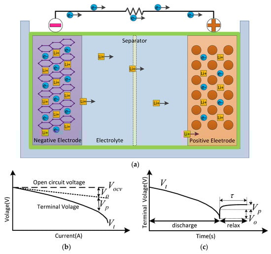
Figure 1.
(a) The discharge process of a typical lithium-ion battery. (b) open-circuit voltage (OCV), ohmic resistance voltage, and polarization voltage as functions of discharge current. (c) The relaxation process of the lithium-ion battery, where is the relaxation time.
The equivalent circuit model is widely used in battery management systems to describe the dynamics of the battery due to its clear physical meaning and balance between computational accuracy and complexity [6,7,21]. Over the past decade, researchers have proposed many kinds of equivalent circuit models, such as the Rint model [22], Thevenin model [23], PNGV model [24], and GNL model [25]. Comparing the SOC estimation accuracy and robustness of the above different equivalent circuit models, Lai, Zheng and Sun [9] and Hu, et al. [26] found that the estimation accuracy does not always improve with the increase of the capacitive resistance network. In contrast, the higher-order equivalent circuit models are more prone to overfitting and reduce their robustness. They may only perform well under test conditions but are poor in noisy environments. Then, the Thevenin model is used in this paper to describe the lithium-ion battery, as shown in Figure 2.
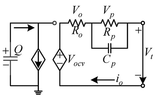
Figure 2.
The Thevenin model.
is the OCV, is the terminal voltage, is the voltage drop caused by ohmic resistance, is the polarization voltage drop, is the current, is the internal ohmic resistance, and are the polarization resistance and the polarization capacitance, respectively.
The model equations can be described as follows:
After discretization:
where donates sampling interval, which is set to 1s in this paper. is the measured terminal voltage at time . is the polarization voltage. is the OCV at time . The mapping relationship between SOC and OCV is determined by the OCV curve in the model-based observer SOC estimation method. Therefore, the accuracy of the OCV curve is critical for SOC estimation.
2.2. Experimental Setup
The AW–IMR14500 lithium-ion batteries are used in this paper. The cathode material is LiCoO2, and the anode material is graphite. The basic specifications of the cells are given in Table 1. The TIBQ27GDK000EVM system is used to test the cells, and ESPEC is used to maintain a constant ambient temperature. The tests were carried out in three cells to ensure reproducibility. The test cells all reached the standard discharge cutoff current/voltage and were fully relaxed to ensure the same initial discharge conditions before each test.

Table 1.
Battery details.
The tests consist of the incremental OCV test, the low-current OCV test, and the dynamic test. Constant current discharge and relaxation operations are alternated in the incremental OCV test. Furthermore, the discharge current set to 1C (700 mA), and the relaxation time is set 2 h for each release of 35 mAh (5% SOC). The test stops when the cell reaches the discharge cutoff voltage in the last discharge process and then relax for 2 h. The low current OCV test uses a constant current discharge mode setting the discharge current to C/50 (35 mA). The test stops when the cell reaches the discharge cutoff voltage and then relaxes for 2 h. Dynamic discharge current and relaxation operations are alternated in the dynamic discharge test. The dynamic discharge process is set to continuously discharge at 700 mA for 200 s, 500 mA for 100 s, 100 mA for 100 s, 400 mA for 100 s, 50 mA for 100 s and 200 mA for 100 s. The relaxation time is set at 2 h. The dynamic test stops when the cell reaches the discharge cutoff voltage in the last constant discharge process and then relaxes for 2 h. The discharge current settings for the above incremental OCV test and the dynamic test are shown in Figure 3.
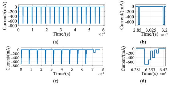
Figure 3.
Schematic of the discharge current. (a) Incremental OCV test. (b) Partial zoom view of incremental OCV test. (c) Dynamic discharge test. (d) Partial zoom view of the dynamic discharge test.
3. State of Charge (SOC) Estimation with Fused Open Circuit Voltage (OCV) Curve Based on Unscented Kalman Filter (UKF)
3.1. Method of Constructing Fusion OCV Curve
The OCV curve is part of the cell model and is critical for SOC estimation. However, the polarization effect affects the accuracy of the OCV test results [15]. The incremental test and low-current test are often used to measure the OCV curve. Petzl and Danzer [15] compared their performance in terms of discharge rate, SOC interval, relaxation time. Both Petzl [15] and Zheng, et al. [27] agree that the incremental test is more suitable than the low current test for determining the relationship between OCV and SOC. However, the OCV curve based on the incremental test is usually obtained by polynomial fitting [28,29,30]. There are few control points obtained by the incremental test, and the fitting curve cannot reflect the non-linear electrode features. The low current test can reflect the characteristics of the electrode, but it is difficult to avoid the polarization effect due to the discharge by constant current.
Figure 4a shows the test results of the incremental and low current tests. The incremental test provides 20 control points that are not affected by the polarization effects. The low-current test provides more non-linear characteristic information of the electrode, reflecting the OCV variation with the DOD. However, the polarization effect is evident with the continued discharge. Figure 4b shows the voltage difference between the two test control points:
where is the voltage of the incremental test in the control point, is the corresponding control point voltage of the low-current test, and is the voltage difference.
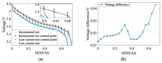
Figure 4.
(a) Incremental test and low current test results. (b) Voltage difference between the two test control points.
The influence of the polarization effect for the low current test is non-linear with the increase of DOD, as shown in Figure 4b.
To weaken the polarization effect while retaining the non-linear characteristics of the electrode, we propose a high-precision OCV curve fusion method based on the low-current test and incremental test data. Firstly, the low-current test control points corresponding to the same discharge depth range are obtained according to the incremental test control points. Then, the voltage difference between the two test control points is calculated, and the ratio of the corresponding voltage difference is taken as the fusion coefficient. Finally, the first-order derivative of the low-current test is taken as the variable, and the final fusion OCV curve is obtained based on the fusion coefficient and the incremental test control points. We first obtain the mapping curve of DOD with OCV and then convert to get the mapping curve of SOC with OCV.
The control points obtained by the incremental test can be expressed as the set , where is the measured OCV at the measured DOD value , is the number of control points. The first measured DOD of the incremental test are obtained at equal DOD intervals, and the last DOD is obtained by the cutoff voltage, where the length might differ from the previous DOD intervals.
The measurements of the low-current test can be expressed as the set , where is the measured OCV at the measured DOD value , is the number of the measurements, and is far greater than . We divide set into sub-intervals according to the DOD of set , and then fuse each interval data. The fusion process is as follows:
Take one DOD interval as an example, the two adjacent control points in set A constitute a semi-open closed DOD sub-interval , which can be described as , .
The corresponding OCV interval is because the OCV is monotonically decreasing during the discharge process. The corresponding DOD sub-interval in set can be determined by , and can be described as . needs to meet the following conditions:
The fused dataset can be expressed as:
where , is obtained by recursion and interpolation, the calculation process is as follows:
Step 1, . Linear interpolation at between the point and , and get the OCV value corresponding to the incremental test control points.
Step 2, Compute the fusion coefficient , where , .
Step 3, Compute the OCV increment .
Step 4, Compute the fused OCV value, .
Step 5, , repeat Step 3–5 until , where .
is the sub-interval fused by the above steps.
The raw test data and fusion results are shown in Figure 5, where the green point set is the fused data. The fused data adjusts the low-current test results based on the control points of incremental test, retains the non-linear characteristic information, and dramatically reduces the polarization effect.
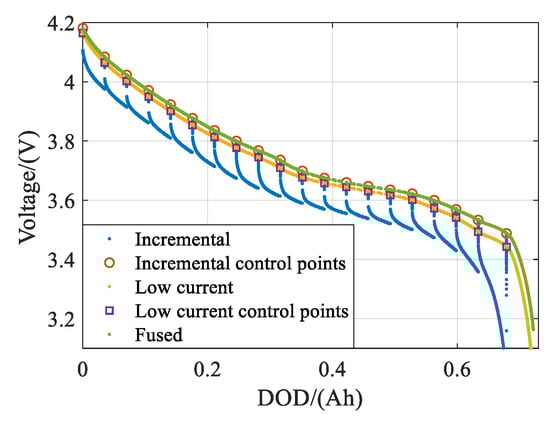
Figure 5.
The OCV fusion results.
The DOD needs to be converted to get the final OCV curve. The conversion formula is as follows:
where is the SOC value in time . is the DOD, and is the cell nominal capacity.
The neural network has better non-linear mapping ability than polynomial fitting. The fusion results have enough data points to fit the OCV curve by using a neural network. The fitting curve is shown in Figure 6. The non-linearity of the OCV curve in the SOC range of 10% to 60% is strong, and the simple polynomial fitting cannot meet the precision requirement. For example, The SOC estimation absolute error of order 5, order 8, order 10 polynomial, and neural network at 40% SOC is 4.016%, 3.062%, 2.221%, and 0.287%, respectively. The experimental results show that the neural network method has a smaller fitting error and is more suitable for fitting the fusion OCV data.
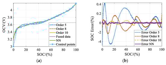
Figure 6.
(a) Comparison of OCV fitting results. (b) Comparison of OCV fitting absolute error.
3.2. Co-Estimation of SOC and Model Parameters Based on UKF
The fused OCV curve improves the lithium-ion battery model accuracy and enhances the stability of the estimation loop. However, the strong non-linearity of the system equation and the unexpected noise still affect the SOC estimation accuracy. In the process of decoupling SOC and model parameters, the traditional EKF method uses Taylor expansion to linearize the system equations by rounding the high-order remainders above the second order, which brings rounding error. While, UKF is a non-exact least variance estimation method, and is very suitable for non-linear state estimation. Its optimal gain matrix is determined by the covariance matrix of the state and measurement quantities. The covariance matrix can be obtained according to the double sigma sample points, which can be determined according to the state equation and the measurement equation.
To joint the estimation of SOC and model parameters by UKF, we designed a state equation including SOC and model parameters. A typical UKF algorithm can be found in reference [31]. The application details of UKF in this paper are as follows.
The discrete state equation and measurement equation can be expressed as:
where and are state and measurement nonlinear functions, respectively. and are independent zero-mean white noise sequences, and their variance arrays are and , is the input sequence.
In this paper, the estimated state is , the measurement is , the system input is . The state function is:
The measurement function is:
where is the OCV determined by OCV curve at time , is the polarization voltage, is the current, , , are the model parameters, is the sampling step, and .
It is assumed that the model parameters change slowly. The UKF algorithm is shown in Algorithm 1.
| Algorithm 1 |
| 1. Initialization , For 2. Compute the simple point at time where is the number of estimation state, is the line of the matrix, and . , , . 3. Compute the value of the one-step forecasting model at time 4. Compute the one-step forecasting sample points 5. Compute and : Where 6. Computer the gain matrix 7. State estimation |
The state estimation sequence contains the model parameters’ identification and the SOC estimation results.
4. Experiment Validation and Discussion
In this section, the proposed fusion OCV curve and state estimation algorithms are compared with other methods, respectively. The pulse constant current discharge (incremental OCV test) and dynamic current discharge test are carried out to validate the effectiveness of the proposed method. The root mean square error (RMSE) and the mean absolute error (MAE) are used to evaluate the SOC estimation results, which are calculated as follows:
where, is the reference value of SOC, is the estimation of SOC, is the number of samples.
4.1. Comparison of SOC Estimation under Different OCV Curve Construction
In this section, the SOC estimation results using the fusion OCV curve, the polynomial OCV curve based on incremental testing, and the OCV curve based on low-current testing are compared and analyzed, respectively. Note that their estimation methods all use the UKF method proposed in Section 3.2.
Figure 7 shows the experimental results of a pulse constant current discharge test. Figure 7a shows the results of the measured terminal voltage, the estimated terminal voltage, and the estimated OCV of the proposed method, respectively. Figure 7b shows the terminal voltage estimation errors. It can be seen from Figure 7a,b that the estimated terminal voltage errors are only 0.005–0.02 V when the current suddenly appears and disappears, yet it is less than 0.001 V during the constant current discharge process. The zoom view in Figure 7a shows that the terminal voltage and OCV drop suddenly when the state switches from relaxation to discharge and then decreases slowly during the discharge; The terminal voltage rises rapidly when the state switches from discharge to relaxation, and slowly during the relaxation process. The estimated OCV converges to the reference value of the terminal voltage slowly. The above results show that the proposed method has an expected OCV estimation result and an excellent tracking performance of terminal voltage.
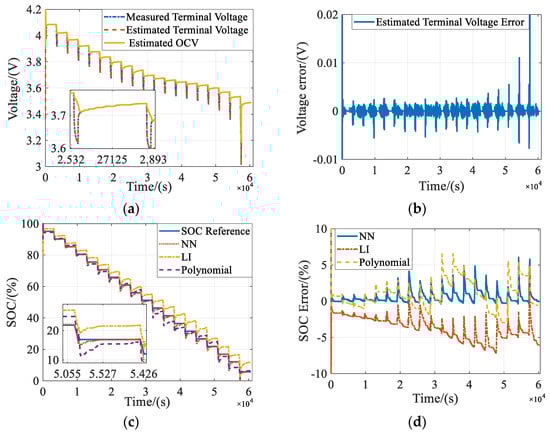
Figure 7.
Comparison of different OCV construction methods in pulse constant current discharge test. (a) Terminal voltage and OCV estimation result. (b) Estimation error of terminal voltage. (c) Comparison of SOC estimation result. (d) Comparison of SOC estimation error.
Figure 7c is the SOC estimation results based on different OCV curve construction methods. It can be seen that the SOC estimation results based on the fusion OCV curve have the least estimation error during the discharge process, and can converge to the reference SOC value in the relaxation stage. The SOC estimation absolute error is shown in Figure 7d. It can be seen that the error based on the fusion OCV curve is least, the absolute estimation error is basically controlled within 4%, and the maximum is 6%. The SOC estimation error based on the low-current test OCV curve increases with the increase of discharge time. Furthermore, the SOC estimation results cannot converge to the reference value in the relaxation stage, which is caused by the polarization effect. The SOC estimation error based on the increment test OCV curve does not accumulate with the discharge time, but the estimation results cannot converge to the reference value accurately in the relaxation stage. This is due to the fact that the increment test OCV curve cannot describe the OCV local non-linearity accurately.
The numerical comparison of the estimated SOC error is shown in Table 2. It can be seen that the RMSE of SOC estimation results based on the fusion OCV curve is reduced by 1.09–2.96%, and the MAE is reduced by 1–3.08% compared with the other two methods.
Table 2.
Comparison of SOC estimation error for different OCV Curves.
Figure 8 shows the experimental results of the dynamic current discharge test. It can be seen from Figure 8a,b that the estimated terminal voltage errors are 0.001–0.023 V during the dynamic discharge process. The OCV estimation results change with the DOD. Furthermore, the OCV estimation results slowly converge to the measurement of the terminal voltage in the relaxation stage. They are in line with expectations. From Figure 8c, it can be seen that the SOC estimation results based on the fusion OCV curve have the best tracking performance, and can converge to the reference value in the relaxation stage. Figure 8d is the SOC estimation absolute error. It is similar to the pulse constant current discharge test, and the SOC estimation error based on the fusion OCV curve is least. The SOC estimation error based on the low-current test OCV curve will accumulate with the increase of the discharge time. The SOC estimation error based on the increment test OCV curve is significant, and the convergence result of the relaxation stage is biased.
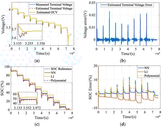
Figure 8.
Comparison of different OCV construction methods in dynamic current discharge test. (a) Terminal voltage and OCV estimation result. (b) Estimation error of terminal voltage. (c) Comparison of SOC estimation result. (d) Comparison of SOC estimation error.
From Table 2, it can be seen that the RMSE of SOC estimation results based on the fusion OCV curve is reduced by 0.26–1.69%, and the MAE is reduced by 0.17–0.76% compared with the other two methods.
The above two test results show that the fusion OCV curve has the highest OCV description accuracy, which almost eliminates the polarization effect on the measurement results and preserves the non-linear characteristics of the electrode. The low-current test is affected by the polarization effect, and the deviation between the OCV measurement and the actual value increases continuously with the DOD, resulting in the steady-state error of the SOC estimation results. The poor accuracy of the incremental test-based OCV curve results in a significant error in the SOC estimation results.
4.2. Comparison of Different SOC Estimation Methods
Figure 9 shows the comparison results between the proposed method with the RLS-EKF [6] and PF [28] SOC estimation method. Note that those estimation methods are all based on the fusion OCV curve. Figure 9a,c are the SOC estimation results of the pulse constant current discharge test and the dynamic discharge test, respectively. It can be seen from the zoom view of Figure 9a,c that the proposed method has higher accuracy of SOC estimation in the discharge process, and can converge to the SOC reference value in the relaxation stage. The SOC estimation accuracy of the RLS-EKF method and the PF method in the discharge process is poor, and there is a sizeable steady-state error between the SOC estimation results and the reference values in the relaxation stage.
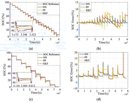
Figure 9.
Comparison of different SOC estimation methods. (a) Comparison of SOC estimation results of the pulse constant current discharge test. (b) The SOC estimation errors of the pulse constant current discharge test. (c) Comparison of SOC estimation results of the dynamic discharge test. (d) The SOC estimation errors of the dynamic discharge test.
Figure 9b,d are the SOC estimation absolute errors of the two tests. It can be seen that the proposed method can maintain a small SOC estimation error in the whole discharge and relaxation process, while the SOC estimation error of the RLS-EKF and PF methods is bigger. This is because the cell internal resistance, the polarization internal resistance as well as the polarization capacitance change greatly when SOC is at 40–50% and below 10%, the PF method cannot adapt to the time-varying model parameters, and the RLS-EKF method cannot accurately estimate the model parameters due to the effect of the environmental noise and measurement noise.
The numerical comparison of the estimated SOC error is shown in Table 3. It can be seen that compared with the other two methods, the RMSE of SOC estimation results of the proposed method is reduced by 1.20–1.67% and the MAE is reduced by 0.97–1.28% in the pulse constant current discharge test, the RMSE is reduced by 0.82–9.18%, and the MAE is reduced by 0.73–0.85% in the dynamic discharge test.
Table 3.
Comparison of SOC estimation error for different estimation methods.
Based on the above results and analysis, it can be seen that the proposed method can achieve accurate SOC estimation. It can maintain a small SOC estimation error in both the discharge process and relaxation stage because of the accurate fusion OCV curve and the joint estimation of SOC and model parameters online.
5. Conclusions
OCV and time-varying model parameters are essential reference variables for the model-based observer SOC estimation method for lithium-ion batteries. In this paper, we propose an OCV curve fusion method based on the increment test and low-current test. The fusion OCV curve is obtained by using the neural network algorithm to fit the fusion data set. The fusion OCV curve retains the non-linear characteristics of the cell electrode while almost eliminating the polarization effect. By designing the state equation including SOC and model parameters, we use the UKF algorithm to achieve a joint online estimation of SOC and model parameters. The experimental results show that the proposed method can achieve accurate and robust SOC estimation. The SOC estimation RMSE and MAE of the fusion OCV curve reached 0.99% and 0.58%, respectively. Furthermore, compared with the RLS-EKF and PF method, the SOC estimation RMSE and MAE reduced by 0.82–9.18% and 0.73–1.28%, respectively.
Since the temperature is a critical factor affecting the cell model parameters, more future works are needed to verify and improve the proposed method. In addition, the effect of the aging process of lithium-ion batteries on the accuracy of SOC estimation is also needed for further research.
Author Contributions
Conceptualization, Y.W. and J.C.; Data curation, Y.W.; Funding acquisition, L.Z.; Methodology, Y.W.; Project administration, L.Z.; Software, Y.W.; Validation, Y.W., J.Z. and S.W.; Visualization, Y.W.; Writing—Original draft, Y.W.; Writing—Review and editing, Y.W., L.Z., J.C., J.Z. and S.W. All authors have read and agreed to the published version of the manuscript.
Funding
This research was funded by the National Natural Science Foundation of China (Nos. 61633008, 61773132 and 61803115).
Conflicts of Interest
The authors declare no conflict of interest.
References
- Farmann, A.; Waag, W.; Marongiu, A.; Sauer, D.U. Critical review of on-board capacity estimation techniques for lithium-ion batteries in electric and hybrid electric vehicles. J. Power Sources 2015, 281, 114–130. [Google Scholar] [CrossRef]
- The Nobel Prize in Chemistry 2019 rewards the development of the lithium-ion battery. Available online: https://www.nobelprize.org/prizes/chemistry/2019/press-release/ (accessed on 11 October 2019).
- Lu, L.G.; Han, X.B.; Li, J.Q.; Hua, J.F.; Ouyang, M.G. A review on the key issues for lithium-ion battery management in electric vehicles. J. Power Sources 2013, 226, 272–288. [Google Scholar] [CrossRef]
- Yang, N.X.; Zhang, X.W.; Li, G.J. State of charge estimation for pulse discharge of a LiFePO4 battery by a revised Ah counting. Electrochim. Acta 2015, 151, 63–71. [Google Scholar] [CrossRef]
- Xing, Y.J.; He, W.; Pecht, M.; Tsui, K.L. State of charge estimation of lithium-ion batteries using the open-circuit voltage at various ambient temperatures. Appl. Energy 2014, 113, 106–115. [Google Scholar] [CrossRef]
- Wei, Z.; Zhao, J.; Zou, C.; Lim, T.M.; Tseng, K.J. Comparative study of methods for integrated model identification and state of charge estimation of lithium-ion battery. J. Power Sources 2018, 402, 189–197. [Google Scholar] [CrossRef]
- Wang, Y.; Zhang, C.; Chen, Z. A method for state-of-charge estimation of LiFePO4 batteries at dynamic currents and temperatures using particle filter. J. Power Sources 2015, 279, 306–311. [Google Scholar] [CrossRef]
- Wei, J.; Dong, G.; Chen, Z. Lyapunov-based state of charge diagnosis and health prognosis for lithium-ion batteries. J. Power Sources 2018, 397, 352–360. [Google Scholar] [CrossRef]
- Lai, X.; Zheng, Y.J.; Sun, T. A comparative study of different equivalent circuit models for estimating state-of-charge of lithium-ion batteries. Electrochim. Acta 2018, 259, 566–577. [Google Scholar] [CrossRef]
- Issac, J.; Qin, J.C.; Saeedifard, M.; Wasynczuk, O. Impact of Current Rate and Temperature on State-of-Charge Estimation of Li-ion Batteries Based on the Extended Kalman Filter. In IECON 2014—40th Annual Conference of the IEEE Industrial Electronics Society; IEEE: New York, NY, USA, 2014; pp. 3122–3128. [Google Scholar]
- Hu, J.N.; Hu, J.J.; Lin, H.B.; Li, X.P.; Jiang, C.L.; Qiu, X.H.; Li, W.S. State-of-charge estimation for battery management system using optimized support vector machine for regression. J. Power Sources 2014, 269, 682–693. [Google Scholar] [CrossRef]
- Chemali, E.; Kollmeyer, P.J.; Preindl, M.; Emadi, A. State-of-charge estimation of Li-ion batteries using deep neural networks: A machine learning approach. J. Power Sources 2018, 400, 242–255. [Google Scholar] [CrossRef]
- Tong, S.; Lacap, J.H.; Park, J.W. Battery state of charge estimation using a load-classifying neural network. J. Energy Storage 2016, 7, 236–243. [Google Scholar] [CrossRef]
- Xiong, R.; Yu, Q.Q.; Wang, L.Y.; Lin, C. A novel method to obtain the open circuit voltage for the state of charge of lithium ion batteries in electric vehicles by using H infinity filter. Appl. Energy 2017, 207, 346–353. [Google Scholar] [CrossRef]
- Petzl, M.; Danzer, M.A. Advancements in OCV measurement and analysis for lithium-ion batteries. IEEE Trans. Energy Convers. 2013, 28, 675–681. [Google Scholar] [CrossRef]
- Meng, J.H.; Ricco, M.; Acharya, A.B.; Luo, G.Z.; Swierczynski, M.; Stroe, D.I.; Teodorescu, R. Low-complexity online estimation for LiFePO4 battery state of charge in electric vehicles. J. Power Sources 2018, 395, 280–288. [Google Scholar] [CrossRef]
- Hu, C.; Youn, B.D.; Chung, J. A multiscale framework with extended Kalman filter for lithium-ion battery SOC and capacity estimation. Appl. Energy 2012, 92, 694–704. [Google Scholar] [CrossRef]
- Dong, G.; Chen, Z.; Wei, J.; Zhang, C.; Wang, P. An online model-based method for state of energy estimation of lithium-ion batteries using dual filters. J. Power Sources 2016, 301, 277–286. [Google Scholar] [CrossRef]
- Meng, J.; Stroe, D.; Ricco, M.; Luo, G.; Teodorescu, R. A Simplified Model-Based State-of-Charge Estimation Approach for Lithium-Ion Battery With Dynamic Linear Model. IEEE Trans. Ind. Electron. 2019, 66, 7717–7727. [Google Scholar] [CrossRef]
- Dong, G.; Wei, J.; Chen, Z.; Sun, H.; Yu, X. Remaining dischargeable time prediction for lithium-ion batteries using unscented Kalman filter. J. Power Sources 2017, 364, 316–327. [Google Scholar] [CrossRef]
- Fotouhi, A.; Auger, D.J.; Propp, K.; Longo, S. Accuracy Versus Simplicity in Online Battery Model Identification. IEEE Trans. Syst. Man Cybern. Syst. 2018, 48, 195–206. [Google Scholar] [CrossRef]
- Nejad, S.; Gladwin, D.T.; Stone, D.A. A systematic review of lumped-parameter equivalent circuit models for real-time estimation of lithium-ion battery states. J. Power Sources 2016, 316, 183–196. [Google Scholar] [CrossRef]
- Ding, X.F.; Zhang, D.H.; Cheng, J.W.; Wang, B.B.; Luk, P.C.K. An improved Thevenin model of lithium-ion battery with high accuracy for electric vehicles. Appl. Energy 2019, 254, 8. [Google Scholar] [CrossRef]
- Liu, C.; Liu, W.; Wang, L.; Hu, G.; Ma, L.; Ren, B. A new method of modeling and state of charge estimation of the battery. J. Power Sources 2016, 320, 1–12. [Google Scholar] [CrossRef]
- He, H.; Xiong, R.; Guo, H.; Li, S. Comparison study on the battery models used for the energy management of batteries in electric vehicles. Energy Convers. Manag. 2012, 64, 113–121. [Google Scholar] [CrossRef]
- Hu, X.; Li, S.; Peng, H. A comparative study of equivalent circuit models for Li-ion batteries. J. Power Sources 2012, 198, 359–367. [Google Scholar] [CrossRef]
- Zheng, F.D.; Xing, Y.J.; Jiang, J.C.; Sun, B.X.; Kim, J.; Pecht, M. Influence of different open circuit voltage tests on state of charge online estimation for lithium-ion batteries. Appl. Energy 2016, 183, 513–525. [Google Scholar] [CrossRef]
- Chen, Z.; Sun, H.; Dong, G.; Wei, J.; Wu, J. Particle filter-based state-of-charge estimation and remaining-dischargeable-time prediction method for lithium-ion batteries. J. Power Sources 2019, 414, 158–166. [Google Scholar] [CrossRef]
- Dong, G.; Wei, J.; Zhang, C.; Chen, Z. Online state of charge estimation and open circuit voltage hysteresis modeling of LiFePO4 battery using invariant imbedding method. Appl. Energy 2016, 162, 163–171. [Google Scholar] [CrossRef]
- Yang, H.; Sun, X.; An, Y.; Zhang, X.; Wei, T.; Ma, Y. Online parameters identification and state of charge estimation for lithium-ion capacitor based on improved Cubature Kalman filter. J. Energy Storage 2019, 24, 100810. [Google Scholar] [CrossRef]
- Julier, S.J.; Uhlmann, J.K. Unscented filtering and nonlinear estimation. Proc. IEEE 2004, 92, 401–422. [Google Scholar] [CrossRef]
© 2020 by the authors. Licensee MDPI, Basel, Switzerland. This article is an open access article distributed under the terms and conditions of the Creative Commons Attribution (CC BY) license (http://creativecommons.org/licenses/by/4.0/).